Classifying human activities through machine learning

(1)

Classifying human activities through

machine learning

Klassificera mänskliga aktiviteter genom machine learning

Jakob Lannge & Ali Majed

Computer Science Bachelor’s thesis 15 credits

Supervisor: Blerim Emruli

Examinator: Radu-Casian Mihailescu Date of final seminar: 30/5-2018

(2)

(3)

Abstract

Classifying Activities of daily life (ADL) can be used in a system that monitor people’s activities for different purposes. For example, in emergency systems. Machine learning is a way to classify ADL with high accuracy, using wearable sensors as an input. In this paper, a proof-of-concept system consisting of three different machine learning algorithms is evaluated and compared between tree different datasets, one publicly available at (Ugulino, et al., 2012), and two collected in this paper using an android device’s accelerometer and gyroscope sensor. The algorithms are: Multiclass Decision Forest, Multiclass Decision Jungle and Multiclass Neural Network. The two sensors used are an accelerometer and a gyroscope. The result shows how a system can be implemented using Azure Machine Learning Studio, and how three different algorithms performs when classifying three different datasets. One algorithm achieves a higher accuracy compared to the machine learning model initially used with the Ugolino data set.

Sammanfattning

Klassificering av dagliga aktiviteter (ADL) kan användas i system som bevakar människors aktiviteter i olika syften. T.ex., i nödsituationssystem. Med machine learning och bärbara sensor som samlar in data kan ADL klassificeras med hög noggrannhet. I detta arbete, ett proof-of-concept system med tre olika machine learning algoritmer utvärderas och jämförs mellan tre olika dataset, ett som är allmänt tillgängligt på (Ugulino, et al., 2012), och två som har samlats in i rapporten med hjälp av en android enhet. Algoritmerna som har använts är: Multiclass

Decision Forest, Multiclass Decision Jungle and Multiclass Neural Network. Sensorerna som har använts är en accelerometer och ett gyroskop. Resultatet visar hur ett konceptuellt system kan byggas i Azure Machine Learning Studio, och hur tre olika algoritmer presterar vid klassificering av tre olika dataset. En algoritm visar högre precision vid klassning av Ugolino’s dataset, jämfört med machine learning modellen som ursprungligen används i rapporten.

Keywords: machine learning, activity of daily life, ADL, supervised learning, multiclass decision

forest, multiclass decision jungle, multiclass neural network, cross validation, Azure, Android, Java, gyroscope, accelerometer

(4)

Acknowledgements

We would like to thank Blerim Emruli, our supervisor, for guiding us and giving us great inspiration throughout the thesis, especially within the machine learning world. It has been a great help.

(5)

T

ABLE OF CONTENT

1 Introduction ... 1 1.1 Background ... 1 1.2 Research aim ... 1 1.3 Limitations ... 2 2 Theory ... 2 2.1 Accelerometer ... 2 2.2 Gyroscope ... 2 2.3 Machine Learning ... 2

2.3.1 Azure Machine Learning Studio ... 3

2.3.2 Training, validation and test data ... 4

2.3.3 Multiclass classification algorithms ... 5

2.3.4 Pearson’s correlation coefficient ... 7

2.3.5 Metrics for Evaluating Classifiers Performance ... 7

3 Related Work ... 9

3.1 A Study on Multiple Wearable Sensors for Activity Recognition ... 9

3.2 Activities of Daily Living and Falls Recognition and Classification from the Wearable Sensors Data ... 10

3.3 Wearable Computing: Accelerometers’ Data Classification of Body Postures and Movements ... 10

4 Method ... 12

4.1 Nunamaker methodology ... 12

4.1.1 Construct a conceptual framework ... 12

4.1.2 Develop a system architecture ... 12

4.1.3 Analyze and design the system ... 12

4.1.4 Build the system ... 12

4.1.5 Observer and evaluate the system ... 12

4.2 CRISP-DM Model ... 12 4.2.1 Business Understanding ... 12 4.2.2 Data Understanding ... 12 4.2.3 Data Preparation ... 13 4.2.4 Modeling ... 13 4.2.5 Evaluation ... 13

(6)

4.2.6 Deployment ... 13 5 Result ... 14 5.1 System ... 14 5.1.1 Transmission of data ... 15 5.1.2 Sensor ... 15 5.1.3 Device ... 15 5.1.4 Software ... 15 5.1.5 Data collection ... 17 5.1.6 Test case ... 18

5.2 Machine learning model... 18

5.2.1 Hyper-parameter algorithm tuning ... 19

5.2.2 Data pre-processing ... 26

5.2.3 Evaluation methods and measures ... 28

5.3 Evaluation result ... 30

5.3.1 Ugolino machine learning model ... 30

5.3.2 Azure machine learning model ... 33

5.3.3 Analyse ... 38

5.3.4 Azure machine learning Android accelerometer data set... 38

5.3.5 Analyse ... 42

5.3.6 Azure machine learning android gyroscope dataset ... 43

5.3.7 Analyse ... 47 5.4 Comparison of models ... 48 6 Discussion ... 48 6.1 Method discussion ... 48 6.2 Result discussion ... 49 6.3 Dataset discussion ... 49

7 Conclusion and future work ... 50

7.1 Answering the Research question ... 50

7.2 Contributions ... 50

7.3 Future work ... 51

(7)

1 I

NTRODUCTION

Below follows a background to the problem domain, and the challenges. In this section the research aims and the limitations of this thesis are described.

1.1 B

ACKGROUND

The development of systems capable of detecting and classifying Activities of Daily Life (ADL) has increased in the last years in order to track human activities. The demand for intelligent surveillance systems within the healthcare industry, especially for physical activities, has increased with the rapid growth of the population of the elderly in the world (Mubashir, et al., 2013). This research area is called Human Activity Recognition (HAR) and aims to assist in the development of emergency systems or other assistive technologies that can help to improve safer living for elderly people. By collecting and analysing data of physical movement it can be used to monitor activity recognition and thus, take action on it.

Modern activity detection systems can be defined as a technical solution, consisting of sensors and hardware with some software. The overall architecture of most of activity detection systems, can according to publications by (Koshmak, et al., 2015) be divided into four different parts. (1) Data acquisition, (2) data processing, (3) activity detection, (4) notification. There are many different variations of the systems in terms of different sensors, software and detection algorithm it uses. Wearable devices sensors, ambience sensors and cameras are three sensor categories normally used during the data acquisition according to (Mubashir, et al., 2013). The paper also states that wearable devices in terms of accelerometers is one of the most popular methods used for measuring physical activities to monitor activity patterns.

A challenge with detecting activities, is that there is a high number of false classifications (also known as true negative, TN), meaning that the algorithm misclassifies the activity. For example, mistaking walking for running. Studies have shown that by using machine learning algorithms during the activity detection, it can improve accuracy and minimize false alarms (Noury, et al., 2007). However, there is also a challenge regarding the available data sets of activities used for training and evaluation of the systems. The data that actually is publicly available within the HAR area is often specific to its own system components and methods, and it is hard to validate its performance.

1.2 R

ESEARCH AIM

The aim of this thesis is to develop a system that uses machine learning algorithms to classify human activities. A system consisting of three different algorithms are trained and evaluated with three different data sets, the publicly available dataset from (Ugulino, et al., 2012), and two data sets collected in this thesis. Thus, an Android client capable of collecting and transmit data from its accelerometer and gyroscope is developed. The different results are then analysed. The following research questions will be answered in this thesis:

 RQ1: How can a system with the capability of collecting and classifying several different ADL activities through Machine Learning be implemented? (Generic question)

(8)

2

 RQ2: How does performance metrics between the machine learning models used in the Ugolino´s paper, differentiates against the machine learning model developed in RQ1, when it is trained and evaluated with the same dataset?

 RQ2: How does the accelerometer and the gyroscope data set collected in RQ1, differentiates in terms of performance metric, when trained and evaluated by the machine learning model implemented in RQ1?

1.3 L

IMITATIONS

 The machine learning model implemented in this paper is developed on the Azure Machine Learning platform.

 The system is only tested on the public data set from Ugolino, and the two data set collected in this thesis.

2 T

HEORY

The following section describes the key technologies and theory the thesis is based, on in order for the reader to understand the thesis.

2.1 A

CCELEROMETER

An accelerometer is a sensor that measures the acceleration of a body. When an accelerometer is in falling towards the center of Earth, it will measure an acceleration of zero, and when it is resting on a flat surface it will measure an acceleration upwards that is equal to the gravity effecting the body, in our case on earth it would be 9.81 m/s2_{. The sensor determines the} acceleration by measuring the force applied to the sensor, then a calculation is made using the relationship between force and acceleration (Allan, 2011).

2.2 G

YROSCOPE

A gyroscope is used to measures the angular velocity. With the angular velocity the rotational motion and changes in orientation can be determined. It is a spinning wheel that can assume any orientation around its rotation axis. The spinning wheel is not affected by tilting or rotation, instead it maintains its orientation duo conservation of angular momentum (Allan, 2011).

2.3 M

ACHINE

L

EARNING

Machine learning is a technology within data science “that uses statistical techniques to give computer systems the ability to learn with data, without being explicitly programmed” (Samuel, 1959). It uses data as input and through the use of statistical algorithms it finds certain patterns in the data and maps this to new, unknown data in order to make correct predictions.

There are different types of machine learning categories, depending on what the model should be able to produce, and what kind of data that is used. Typically, these tasks are classified into three distinct categories:



Supervised learning:

Supervised machine learning means that the input data the model is being trained with, is known. The model analyses the known data by looking at the characteristics (generalization) of it and uses this to predict future unknown data. This is one of the most common machine learning principles. It includes algorithms such as regression and classification algorithms. A regression problem is when the desired

(9)

3

output is a number, such as length or distance. In classification problems, the desired output is a category, such as colours or names (Han, et al., 2012).



Unsupervised learning:

Opposite to supervised learning, unsupervised learning is when the model is not being trained by labelled data. Instead the goal is to cluster or find similar patterns in the data without supervised training.



Reinforcement learning:

The third category is called reinforcement learning, similar to unsupervised learning it does not get trained by any known data, or only partly. However, as it progresses is learns. By taking action for every data point given, when the action is right a positive signal is given, if the action is wrong a negative signal is given. The correct actions can then be fed back to the model as training data thus making it better and better to predict new unseen data. It is a learn-by-doing model with built-in “reward” feedback-system, either manual or automatic such.

2.3.1 Azure Machine Learning Studio

Azure machine learning is a platform combined of PaaS and SaaS services available in Microsoft Azure cloud. The service provides out-of-the-box modules for building machine learning models that can be built and modified inside a cloud-based studio accessible from a web browser, the studio is free to use and accessed by a paid or free user subscription. It is designed through a drag-and-drop mode with manual configuration inside some of the modules. The studio provides internal, as well as third-party tools to perform data actions such as feature extraction, pre-processing and analysis. These modules can be used to import datasets, build and train different machine learning algorithms, and evaluate the model’s performance by cross-validation and confusion matrix. See figure 1 to get an overview over the studio.

(10)

4

More importantly the studio provides built-in machine learning algorithms which are ready for use. For multiclass models, the studio supports four different algorithms, in this paper, three of them are used. Multiclass Decision Forest, Multiclass Neural Network and Multiclass Decision Jungle.

2.3.2 Training, validation and test data

A machine learning model depends on a data set, a data set contains several features and instances from a specific problem domain. In classification models, the algorithm uses the data set to train itself to the point where it can successfully describe and distinguish data classes or labels, (Han, et al., 2012). For example, consider a data set that contains 4 different features (columns), each with 10,000 instances (rows) each. The three first features contains numeric values, and the fourth one contains a category, for example the name of different car brands. The point of the training stage is to map the numeric data from the data set that corresponds to a specific category.

Later when new data are fed to the model, it can use the historical data which it has been previously trained with, to make predictions on the unknown data. By measuring how accurate the model predicts the new data (test data) the performance of the machine learning model can be evaluated.

Most algorithms used in the machine learning models always has a few key hyper-parameters that can be selected before applying the model. (Chicco, 2017). These parameters should be tuned by a so-called validation data set together with the training data to achieve the highest performance of the model in terms of trying out different algorithm parameters. When the best parameters are found, the final evaluation of the model can be performed by using the test data set.

The training data, validation data and test data are all normally obtained from one initial data set by splitting it up into different parts. It is important however, that the test data is not used at all during the training of the model, this would affect the performance of the model negatively. (Witten, et al., 2016). Instead the data set should be split up into two or more parts, separating between training and test data. This way the algorithm can be trained with one part and validated with another independent part of the data.

In the popular cross-validation technique, the holdout method, this process is done

automatically. It randomly splits the initial dataset into two partitions, one for training, and the second one is kept aside for testing, in a holdout folder. The hold-out method is a classic way used for evaluating a machine learning model, as it keeps the test data independent from the training data. The ratio of each set can be configured, for example a ratio of 0.5 corresponds to that 50% of the all the instances in the data set will be used for training, and the remaining 50% instances will be used for testing. However, splitting the data set with a 50:50 ratio, is generally not ideal. It is better to maximise the amount of data for training and leave a smaller portion out for testing, to obtain a good performance. But if the initial data set is small, this limits the

amount of data that can be used for training, testing and if applied, validation (Witten, et al., 2016). Also, the proportion of the samples are not well divided, one certain class could for example end up in the training set and not in the test set.

This problem is called underfitting and usually happens if the training dataset is too small, it

will affect the model’s performance negatively. A model fails to find the underlying pattern in the learning data and struggles to predict the correct output on new data.

Overfitting is another problem that occurs in machine learning, on the contrary to

(11)

5

to “memorize” the training set, including noise and random fluctuations which are not relevant to categorize future data.

2.3.3 Multiclass classification algorithms

In a classification machine learning model, the goal is to classify different given categories or labels. It is a supervised learning method, where an algorithm is used to estimate the function between the input variables (x), and the output variable (Y). See figure below:

𝑌 = 𝑓(𝑥)

When a function is found, the algorithm should be able to make predictions of Y for new values of x. The output is a category, or class that the algorithm previously has learned. There are several classification algorithms, however some of them are meant predict multiple different classes, compared to binary models which only outputs one or two classes. For example, is this person over 40 years old? Or, is this colour black? This represents a binary output, negative or positive. Machine learning models can output more than two classes are often referred to as multiclass classification algorithms. The output can for example be, what is the age of this person, 10, 20, 30 or 40 years old? Or, what colour is this, black, red, green or yellow? 2.3.3.1 Multiclass Decision Forest

Multiclass decision forest is an algorithm based on the popular Decision Tree learning method. The method builds binary trees and then traverses through the nodes. “Each node in the

decision tree specifies a test of some attribute of the query instance, and each branch descending from that node corresponds to some of the possible values for this attribute”, (Maja, 2005). Each instance is starting at the root node of the tree. In each tree, a sequence runs through every node until a leaf node is reached, which is the decision. In this project the open source Azure Machine Learning studio is used, it provides an ensemble of decisions trees and voting on the most popular output class.

Azure machine learning studio allows for the following parameters of this algorithm to be tuned, (the set settings are default in Azure ml studio).

 Resampling method: Bagging or replicate

The method used to create the individual trees. Bagging is a type of bootstrap

aggregating where each tree is grown on a new sample, created by randomly sampling the original dataset with replacement until the dataset has the size of the original. In replicate mode, each tree is trained on exactly the same input data.

 Create trainer mode: Single parameter The way the model is being trained.  Number of decision trees: 8

The number of decision trees created in the ensemble. The more trees, the longer training time.

 Maximum depth of the decision trees: 32 The maximum depth of any decision tree.  Number of random splits per node: 128

The number of splits to use when building each node of the tree.  Minimum number of samples per leaf node: 1

The number of cases that must meet the same conditions before any leaf nodes are created.

 Allow unknown values for categorical features: check

If this is unselected, the model can only accept values that are present in the training dataset.

(12)

6 2.3.3.2 Multiclass Decision Jungle

Multiclass Decision Jungle is an extension to decision forests, by allowing tree branches to merge into directed acyclic graphs, (DAG). It requires less memory usage and better generalization; however, the training time is higher than decision forest models (Han, et al., 2012).

As for the hyper-parameters in the Multiclass Decision Jungle method, they are similar to the decision forest algorithm, but with some minor differences. The following ones are default in Azure ML studio and available for tuning.

 Resampling method: Bagging

 Create trainer mode: Single parameter  Number of decision DAGs: 8

 Maximum depth of the decision DAGs: 32  Maximum width of the decision DAGs: 128

The number of splits to use when building each node of the tree.  Number of optimization steps per decision DAG layer: 2048

The number of iterations over the data to perform when building each DAG.  Allow unknown values for categorical features – check

2.3.3.3 Multiclass Neural Network

Multiclass Neural Network is another algorithm that can be used in a supervised learning model. The neural network principle is inspired by human or animal brains. Such systems learn by input data, and then considers outputs based on its own attributes it evolves from the input data. A neural network model consists of interconnected layers, weighted edges and nodes called artificial neurons, comprised to a graph connects the different layers. Inputs are the first layer, and output are the last layers. The neurons can send signals between each other and the direction of the signals starts at the inputs and works its way through the layers out to the output. Based on the input a value is calculated at each layer and node. Neural networks are commonly used in complex computer vision tasks, such as speech recognition or pattern recognition (Han, et al., 2012).

The following hyper-parameters are default for the multiclass neural network algorithm in Azure ML studio, and available for tuning.

 Create trainer mode: Single parameter

 Hidden layer specification: Fully-Connected case

This is default neural network architecture, this specifies how the layers are connected.  Number of hidden nodes: 100

Specifies the number of hidden nodes in the neural network.  The learning rate: 0.1

Defines the size of iteration through the layers. A smaller number can lead to a faster model but can overshoot some valuable information.

 Number of learning iterations: 100

The maximum number of time the network should iterate through the input data.  The initial learning weights diameter: 0.1

Specify the node weights at the start of the learning process. 0.1 is default and chosen for simplicity. The higher weight the nodes start with, the more data needs to be processed initially.

 The momentum: 0

Defines how much weight to apply to the nodes during learning from previous iterations.  The type of normalizer:

(13)

7

Selects the method for normalization of the input data’s features.  Shuffle examples: check

When selected the cases are shuffled between iterations and training of the algorithm.  Allow unknown categorical levels: check

If deselected the model only accepts values contained in the training dataset, if selected it creates groups for unknown values in the training and validation dataset.

2.3.4 Pearson’s correlation coefficient

A data set contains several attributes but it is possible that not all the attributes are relevant when training a machine learning model. To identify the attributes that are not relevant, a processes of statistical test is applied on the input, given a specified output, to determine the attributes that have more predictive power.

Using Pearson’s correlation coefficient (Gravetter, et al., 2017) is one way to identify the predictive power of an attribute. It returns the strength of correlation between two variables. Pearson’s correlation coefficient is calculated by taking the covariance of two variables and dividing by the product of their standard deviation. The result is a value between +1 and -1, where 0 means that there is no correlation, +1 means that there is total correlation and -1is that there is a negative correlation.

2.3.5 Metrics for Evaluating Classifiers Performance

Measures for assessing how “well” and how accurate the machine learning model predicts classes is essential, it is used to evaluate the performance of the model and compare it to others.

10-fold cross-validation is a cross-validation technique, strongly connected to the hold-out

method. Instead of splitting the dataset up into two partitions, it divides the data randomly into different 10 folds, with each class approximately equally represented. 9 of 10 parts are used for training, and the last nine-tenth is hold-out for testing. This process is repeated 10 times so that in the end, the learning process is executed 10 times on different training sets and each part has been used exactly once for testing. This helps to minimize underfitting as well as overfitting in a machine learning model, and to evaluate its performance in a truthful way. The technique is the standard way of measuring performance metrics and the quality of a machine learning model (Witten, et al., 2016).

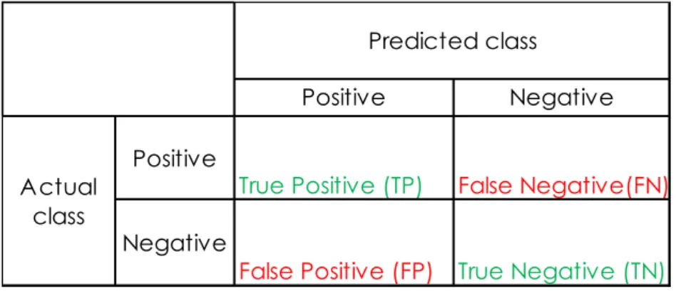
A confusion matrix is a table for summarizing the performance of a classification model. It

shows number of correctly and incorrectly predicted classes, against the actual classes in the test data, see table 1. It is used to view the different possible outcomes, which are later used calculate the model’s performance. The number of True Positive (TP), False Positive (FP), True Negative (TN) and False Negative (FN).

 TP is the number of positive predictions that are actually positive (correctly classified).  TN is the number negative predictions that are actually negative (correctly classified).  FP is the number of positive predictions that are actually negative (incorrectly

classified).

(14)

8

Table 1: Definition of a Confusion Matrix

The confusion matrix is often used in classification models, either in binary models or multiclass models. In a multiclass model however, the confusion matrix can be visualized as in table 2, where each class is represented with a column and as a row, in this case there is five classes (Witten, et al., 2016). The column represents the predicted class that the model outputs, and the row represents the actual class. The number of TP are shown in the diagonal, and the remaining boxes are considered as errors and are used to find out the number of FP, FN and TN as it differs from a binary classifier. The total number of each outcome can be calculated as:

 TP = the number of TP’s for a class is shown as TP.

 TN = the number of TN’s for a class is the sum of all columns and rows, excluding that class´s column and row.

 FP = the number of FP’s for a class is the sum of values in the corresponding column, excluding the TP.

 FN = the number of FN’s for a class is the sum of values in the corresponding row, excluding the TP

Table 2: Confusion matrix for five classes Predicted class

Actual class Class A Class B Class C Class D Class E

Class A TP E E E E

Class B E TP E E E

Class C E E TP E E

Class D E E E TP E

Class E E E E E TP

Accuracy is a classifiers overall recognition rate and measures the percentage of all the

correctly classified (predicted) instances from the whole test set. That is, all instances of TP, plus all the instances of TN, divided by the total numbers of outcome (Han, et al., 2012). It´s

calculated as:

𝐴𝑐𝑐𝑢𝑟𝑎𝑐𝑦 = 𝑇𝑃 + 𝑇𝑁

𝑇𝑃 + 𝑇𝑁 + 𝐹𝑃 + 𝐹𝑁

(1)

Precision is a measure that shows the proportion of correctly classified classes, to the sum of

correct classifications and the falsely predicted positive instances. It is used to measure a classification models exactness, i.e., the percentage of positive classes are labelled as such (Han, et al., 2012). The equation looks like:

Positive

True Positive (TP) False Negative(FN)

Negative

False Positive (FP) True Negative (TN)

Actual class

Predicted class

(15)

9 𝑃𝑟𝑒𝑐𝑖𝑠𝑖𝑜𝑛 = 𝑇𝑃

𝑇𝑃 + 𝐹𝑃

(2)

Recall is a measure of a model’s completeness, also known as the sensitivity. It is used to calculate the true positive rate, which is the proportion of positive classes that are correctly identified (Han, et al., 2012). The equation looks like:

𝑅𝑒𝑐𝑎𝑙𝑙 = 𝑇𝑃 𝑇𝑃 + 𝐹𝑁

(3)

F-measures is the weighted average of precision and recall, it is used to look at the relationship between precision and recall (Han, et al., 2012). The equation looks like:

𝐹 = 2 ⋅ 𝑝𝑟𝑒𝑐𝑖𝑠𝑖𝑜𝑛 ⋅ recall 𝑝𝑟𝑒𝑐𝑖𝑠𝑖𝑜𝑛 + 𝑟𝑒𝑐𝑎𝑙𝑙

(4)

3 R

ELATED

W

ORK

This chapter presents the most relevant papers to this thesis, found through the literature review. Below they are summarized and explained how they relate to this thesis.

3.1 A

S

TUDY ON

M

ULTIPLE

W

EARABLE

S

ENSORS FOR

A

CTIVITY

R

ECOGNITION

The paper (Huang, et al., 2017), used an accelerometer with a three-dimensional Cartesian coordinate system. Three sensors were used, they were attached to the waist, left wrist and the right wrist. The purpose was to collect motion data for activity recognition and measure the impact of using several sensors of the same type.

Supervised machine learning algorithms were used to classify the activities. The three machine learning algorithms that were used are called random forest, decision three and support vector machines. The activities were classified into five categories: laying down, walking, standing up, sitting and dining.

The sensor that was used can achieve a sample rate up to 200 Hz. The data was sampled at 75 Hz and sent with Bluetooth to a laptop. Two persons were used for the data collection. They were asked to perform different activities within a specific time interval, the total time spent on collecting data was 121 minutes (12 minutes standing, 11 minutes laying down, 15 minutes walking, 43 minutes dining and 40 minutes sitting). The dining activity involves eating and drinking while sitting down. The walking activity involves walking along a corridor, walking up and down stairs. For the standing activity the subjects were supposed to stand on the same spot and were only allowed to talk. The last activity was laying on a bed, and the subjects were permitted to change their posture whenever they wanted.

The accuracy of the classifiers was evaluated using 10-fold cross-validation. Their results show that using multiple sensors yields a higher accuracy at 81.1 % compared to 73.2 % from a single sensor attached to a non-dominant wrist, but multiple sensors almost achieved the same results when the subject attached a single sensor to the dominant wrist, the accuracy was then 80 %. Decision three gave the best results with an accuracy of 81.1 %.

This paper is relevant to this thesis because it shows that the placement of the sensors can affect the accuracy for classifying activities.

(16)

10

3.2 A

CTIVITIES OF

D

AILY

L

IVING AND

F

ALLS

R

ECOGNITION AND

C

LASSIFICATION

FROM THE

W

EARABLE

S

ENSORS

D

ATA

The paper (Ivascu, et al., 2017), compares the accuracy of different machine learning algorithms for recognizing physical activities. The data used to train the algorithm is publicly available and is provided by the University of Milano Bicocca. The data is gathered using a Samsung Galaxy Nexus, using an accelerometer with a three-dimensional Cartesian coordinate system, with a sample rate of 50 Hz. 9 activities and 8 types of falls were performed by 30 subjects. A total of 7013 samples were collected.

The activities that the subjects performed were: going upstairs, going downstairs, sitting on a chair, standing from a sitting position lying down, getting up from bed, jumping, walking,

running, falling forward, falling backward, falling left, falling right and sitting down. The subjects performed each activity five times while wearing the sensor on the left and right (split evenly) pocket on their trousers. Each dataset was manually labelled.

The machine learning algorithms used to classify the physical activities are the following: K-Nearest Neighbor, Gaussian naïve Bayes, Support Vector Machines, Decision Tree, Adaptive Boosting and Random Forest. There was also a deep learning algorithm called Deep Neural Network.

Three cross-validation methods were used to measure the accuracy. The hold-out method showed that k-Nearest Neighbor gave the highest accuracy with 86.48 % for physical activities and 60.98 % for falls. Using 5-fold cross-validation, Deep Neural Network performed best, with an accuracy of 86.30 for physical activities and 50.08 for falls. The Leave-One-Subject-Out method showed that Deep Neural Network performed best for physical activities, with an accuracy of 91.55 % and Random Forest gave the best results for falls with an accuracy of 52.31 %.

This paper is relevant to this thesis because it shows that a relative high accuracy can be achieved with a smartphone and which machine learning algorithm is most suitable.

3.3 W

EARABLE

C

OMPUTING

:

A

CCELEROMETERS

’

D

ATA

C

LASSIFICATION OF

B

ODY

P

OSTURES AND

M

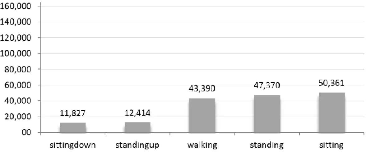
OVEMENTS

In this paper (Ugulino, et al., 2012), a wearable device is built, consisting of four tri-axial accelerometers positioned on the waist, thigh, ankle and arm and used to collect activity data. The sensors are connected to a microcontroller and the data collection was performed on four subjects whom were performing static and dynamic movements. The profiles were diverse, women, men, young adults and one elder.

Total data was collected during an eight-hour period, two hours for each subject. A total of 165 632 samples were collected, approximately 50 000 were collected per each subject except for one, approximately 10 000 samples were collected by this subject.

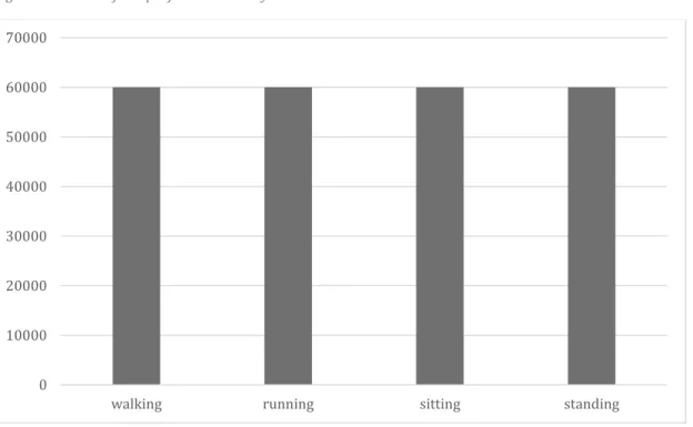
The activities collected are: sitting down, standing up, walking, standing and sitting. Sitting down means going from standing to a sitting position and standing up vice versa. The distribution between the activities and the number of samples can be seen in figure 2.

(17)

11

Figure 2: Number of samples distributed between the classes

After collection, the data undergoes some pre-processing, they were grouped, and derivate features were generated.

 For each accelerometer: Euler angles of roll and pitch and the length (module) of the acceleration vector (called as total_accel_sensor_n);

 Variance of roll, pitch and module of acceleration for all samples in the 1 second window (approximately 8 reads per second), with a 150ms overlapping;

 A column discretizing the module of acceleration of each accelerometer, defined after a statistic analysis comparing the data of 5 classes;

The final dataset contains 19 attributes, whereas 18 of those contains features, and the 19th attribute contains a label (class). See table 3. X1, Y1, Z1 corresponds to sensor 1, and X2 to sensor 2 and so on.

The data set is publicly available for free use at this reference: (Ugulino, et al., 2012).

Table 3: Ugolino’s dataset with 19 attributes

User Gender Age How_tall_in_meters Weight Body_mass_index X1 Y1 Z1 X2 Y2 Z2 X3 Y3 Z3 X4 Y4 Z4 class

String String Int Real int Real Int Int Int Int Int Int Int Int Int Int Int Int string

AdaBoost with 10 iterations and Decision tree learning were used to classify the activities. The results were evaluated using k-fold cross-validation. Using 10-fold cross-validation, an overall recognition performance of 99.4% was achieved. More information about the results are presented in chapter 5.3.1.

This paper is relevant to this thesis because it provides the dataset that is used in this thesis for building the machine learning model. The performance from this papers machine learning model are then compared with result of this thesis’s model, which are generated by different machine learning algorithms.

(18)

12

4 M

ETHOD

Two methods are used, one is used to build a prototype that can collect data from a subject, and the other method is used to build the machine learning models. These two methods are

described in 4.1 and 4.2.

4.1 N

UNAMAKER METHODOLOGY

A prototype is built to collect data from the user. To develop the prototype, the methodology that is presented by Nunamaker (Jay, et al., 1990) was used. The methodology consists of five parts, these parts are explained further in 4.1.1-4.1.5.

4.1.1 Construct a conceptual framework

The first parts consist of defining the problem domain and breaking it down into research questions, this is presented in chapter 1.2. Also, requirements are defined for the prototype that will be used to verify that the data can be collected from the user, the requirements are

presented in 5.1. A literature study is done to gain further knowledge about the parts in the prototype, the results of the literature review is presented in chapter 2 and 3.

4.1.2 Develop a system architecture

This part consists of creating an architectural view of the system that will show the relationships between the different components in the system, this is presented in chapter 5.

4.1.3 Analyze and design the system

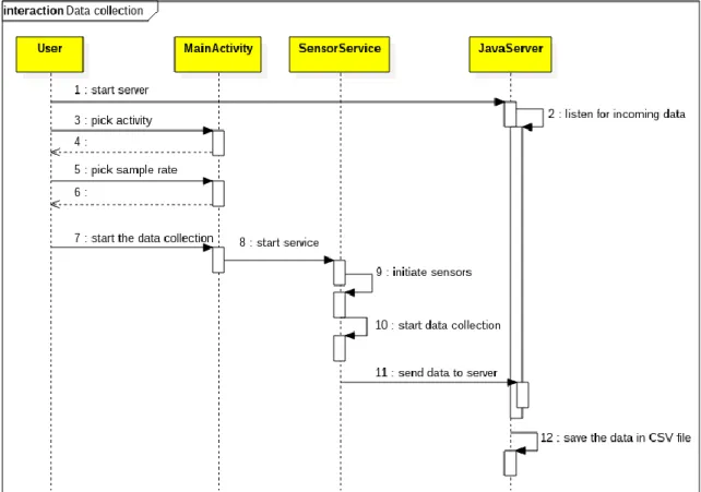
In this part, design specifications are created to be used as blueprint for implementation of the system. A class diagram is created to give an overview of the data structure used to collect data from the user. Also, a sequence diagram is created to show how the data is collected. The class diagram and the sequence diagram can be seen in 5.1.4.

4.1.4 Build the system

In the fourth part of the methodology, the prototype is implemented based on the requirements.

4.1.5 Observer and evaluate the system

In the final part, the prototype is to verify that the requirements have been met. How this is verified can be viewed in 5.1.6.

4.2 CRISP-DM

M

ODEL

To build the machine learning models, a method presented in (Shearer, 2000) is used. It consists of six phase, theses phases are presented in 4.2.1 to 4.2.6.

4.2.1 Business Understanding

The first phase is to understand the objective of the project. This is done in order to understand what data should be collected. The objective of the project can be read in section 1.1.

4.2.2 Data Understanding

The second phase is to collect the data and describe the data. This includes information about the quantity, the number of attributes and information about each attribute and if there are missing values in the dataset or other notable information. Information about collected data can be seen in section 5.1.5 and information about the public dataset can be seen in 3.3.

(19)

13

4.2.3 Data Preparation

This phase covers all the activities to construct the final dataset. This includes cleaning the data from data points that have missing information, constructing new attributes from existing ones if necessary, e.g. by computing new values, and integrate data from other tables. Filtering and feature selection is also made in this phase. The result from this phase can be found in chapter 5.2.2.

4.2.4 Modeling

In the fourth phase, one or more modeling techniques are chosen. These models are then tuned and trained, and test are conducted to measure the quality of the models. The choices of models and how the models are tested is described in section 5.2.1 and 5.2.3.

4.2.5 Evaluation

In this phase the results from the tests are evaluated and an assessment of how well the models achieve their objective. Performance metrics are observed and analyzed. The result of this can be found in section 5.3.

4.2.6 Deployment

In the last phase, a report is produced that consist of results from the other phases. In this case, this thesis is the report.

(20)

14

5 R

ESULT

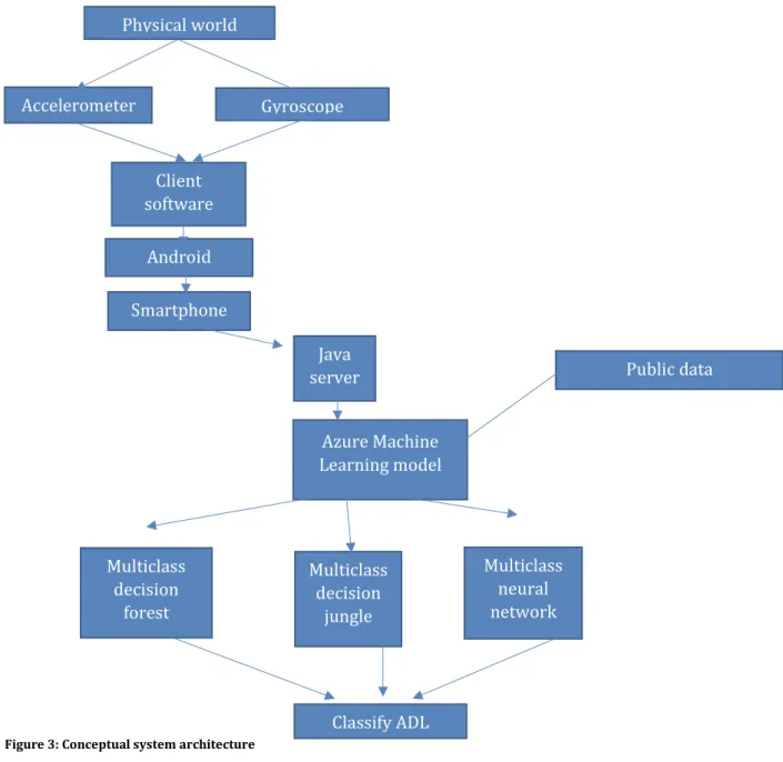
A conceptual architectural view over the system and its components is shown in figure 3. A user performance different activities in the physical world, these activities are measured using an accelerometer and a gyroscope. The measurements are handled by the software on client, which runs on the Android operating system. The client software uses the hardware for the cellular network to transmit the data to the server. The server receives the data and converts it to CSV format so that the models can be trained.

Figure 3: Conceptual system architecture

5.1 S

YSTEM

To build a system that can differentiate between ADL, data from the subjects must be collected. To collect the data, hardware with specific requirements are needed. These requirements defined so that a user can move around freely while the device collects data and sends the data to the server. The requirements are:

Classify ADL Multiclass decision forest Multiclass decision jungle Multiclass neural network Azure Machine Learning model Java server Smartphone Android Client software Accelerometer Gyroscope Physical world Public data

(21)

15

1. The user should not be constrained by their position 2. The device should be able to detect the user’s movement 3. Able to send the collected data to a remote computer

The first requirement means that the user should be able to move just like they do in their ordinary life. More specifically, this means that the user should be able to move indoors and outdoors, walk to their job/school or run in the woods.

The second requirement means that a sensor can detect vertical and horizontal movement from the subject.

The third requirement means that the hardware must be able to send the collected data to a remote computer which may or may not be close to the subject.

5.1.1 Transmission of data

The large amount of data that is collected on the device needs to be transmitted to a remote compute, there the data is used to train the machine learning model. Wi-Fi, Bluetooth and broadband cellular network were considered as potential technologies for transporting the data. The first requirement for data collection states that the subject should not be constrained by their position, meaning that they can travel long distances without worrying about being able to send the data to the remote computer. This requirement eliminates Wi-Fi and Bluetooth,

because they are short-rage technologies. With broadband cellular network the subject can move freely without being constrained by their position, therefore broadband cellular network was chosen to be the technology that transports the data to the remote computer.

5.1.2 Sensor

There are many ways to collect data from the physical world e.g. using accelerometer,

gyroscope, barometer, microphone, camera, iris scanner, fingerprint scanner, thermometer and pulse meter. The most important requirement for the sensor is the second requirement, it says that a sensor should be able to detect movements made by the subject. This leaves

accelerometer, gyroscope and camera for further consideration. But the third requirement states that the subject should be able to move freely eliminates the camera because a camera can only cover a specific area. The accelerometer and the gyroscope meet all the requirements and therefore they were chosen. The values from the gyroscope and the accelerometer are represented with a three-dimensional Cartesian coordinate system.

5.1.3 Device

To get the collected data from accelerometer and the gyroscope to be sent via the broadband cellular network to the remote computer, a smartphone was used. A smartphone is suitable to carry while doing ADL, has the sensors needed for the requirements and has the capability to send the collected data to a remote computer via broadband cellular network. The smartphone that was chosen is a Samsung S8.

5.1.4 Software

The software used to collect the data from the subject consist of software on smartphone and software on a remote computer.

The software on the smartphone runs on the Android operating system, programmed in the Java programming language. Oreo 8.0 is the version used on the Android operating system.

The authors in (Hakim, et al., 2017) were able to classify ADL with a sample rate of 10 Hz. The Samsung S8 is capable of sampling with a higher rate 10 Hz, a choice was made to start with a sample rate of 100 Hz. The software on the smartphone collects the data from the accelerometer

(22)

16

and the gyroscope with a sample rate of 100 Hz. The labelling of data is done manually, before the data collection begins. The desired activity and the number of samples are set on the client. After start is pressed, the client waits 5 seconds before the collection of data begins. This is done, so that the test person has time to put the device in their pocket. After the data has been

collected, it’s stored in the data structure showed in figure 4. The data is then sent to the server using broadband cellular network with the Internet protocol and the TCP transport layer.

Figure 4: Class diagram for the class SensorData

The server runs on a Java virtual machine, using the Java programming language. The job of the server is to listen for incoming data from client, store the incoming data in the data structure showed in figure 5. The user can at any point save the collected data in a CSV. The reason the CSV format was chosen, is because the machine learning module in Microsoft Azure accepts its data as a CSV file. In the sequence diagram in figure 4 show the whole process of collecting data.

(23)

17

5.1.5 Data collection

The choice of activities to evaluate is based on existing public data that is available. This was done so that a comparison can be made between the public data from Ugolino and the data that collected by us.

The activities are: walking, running, sitting and standing. The data is collected during ten minutes for each activity, each activity is sampled 60 000 times during this period, and this can be seen in figure 6. While collecting the data, the smartphone was placed in the subject’s left pocket, with the screen facing the body. The walking activity was conducted by walking for five minutes on asphalt and five minutes on a dirt road. During the sitting activity, the subject could do anything as long as the subject stayed seated on a chair for ten minutes. The subject ran for five minutes on asphalt and five minutes on a dirt road for the running activity. While standing, the subject could move their body as long as they stayed in the same position. A table of how long the data collection lasted for each activity can be seen in table 4.

Table 4: sample time for each activity

Activity Time (minutes)

sitting 10

standing 10

walking 10

running 10

Figure 6: amount of sample for each activity

Each dataset consists of 6 attributes, this can be seen in table 5. The first attribute is called “sensor”, this is the name of the sensor (in this thesis, two sensor are used and they are labelled as accelerometer and gyroscope). The three attributes that are called “x”, “y” and “z” are the collected values for a sensor at a specific time. In the case of the accelerometer, these values represents the acceleration for each axis in a Cartesian coordinate system. In the case of the

0 10000 20000 30000 40000 50000 60000 70000

(24)

18

gyroscope, the angular velocity is measured. The fourth attribute is called “time”, this attribute represents the UNIX timestamp in nanoseconds when the data was collected. The last attribute is called “activity”, this represent the current activity.

Table 5: the attributes for the collected data

sensor x y z time activity

string double double double long string

The dataset is publicly available for free use at this reference: (Lannge & Majed, 2018).

5.1.6 Test case

Table 6 the cases that are used to verify that the requirements for the data collection system are met.

Table 6: test cases for the data collection system

ID Objective Steps Expected result

1 The user should be able to choose

activity The user picks an activity from the GUI The collected data is labelled according to what the user picked in the GUI

2 The user should be able to start the

data collection by pressing a button The users presses a button that will start the data collection

The data collection starts 5 seconds after the users presses the button

3 The device should be able to collect

data from the accelerometer Data collection from the accelerometer starts after the user initiates it from the GUI

Data from the accelerometer is collected

4 The device should be able to collect data from the gyroscope

Data collection from the gyroscope starts after the user initiates it from the GUI

Data from the gyroscope is collected

5 The device should be able to send the collected data from the device to the server

The data is sent to the server after it’s collected

The collected data is received on the server

6 The server should be able to receive

data from the device The server is listening for incoming data and stores it in memory when it arrives

When data is sent, the server is able to receive it

7 The server should be able to save the received data as a CSV-file

After the data is received, the server stores the data in a CSV-file

The received data is stored in a CSV-file

5.2 M

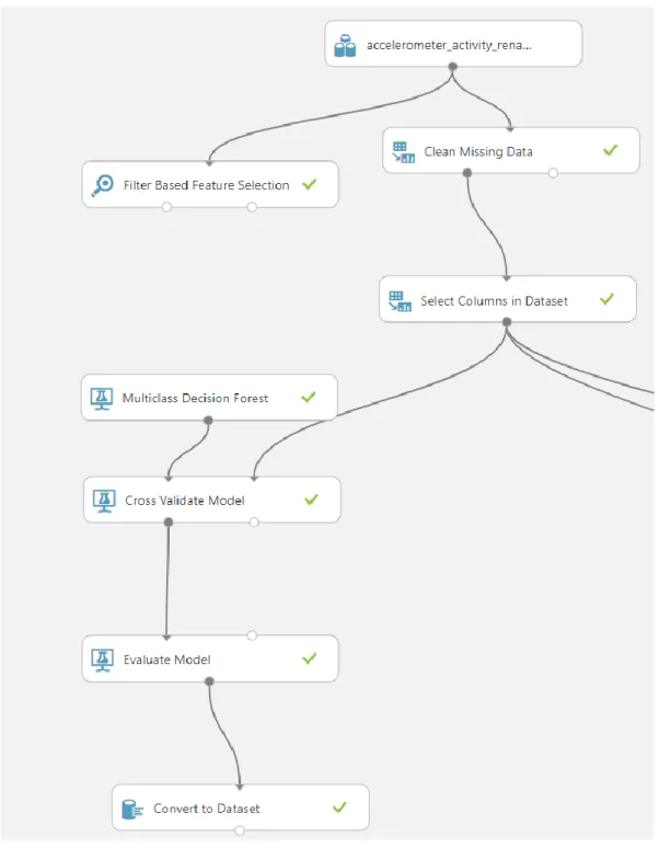
ACHINE LEARNING MODEL

This section describes the result of the machine learning model. It shows how the models is built and configured together with how the collected data is processed. Figure 7 shows an overview of

(25)

19

the model and the modules used when it is configured with the Android accelerometer data set and the multiclass decision forest algorithm.

Figure 7: overview of the model

5.2.1 Hyper-parameter algorithm tuning

Azure machine learning studio allows for parameter tuning per each algorithm, including the ones used in this thesis. As mentioned in the section 2.1.1, tuning is often done during training stage, however preferably with an independent data set.

Tuning is performed by building an independent model which uses the whole data set from Ugolino, then different combinations of key hyper-parameters are changed from each algorithm and tested out, to see which one of them performs best in terms of accuracy. As a limitation, three different combinations is tried out, and not all parameters are changed in each test. The

(26)

20

parameters are changed from the default settings provided in Azure ML studio. Tuning is only made on Ugolino’s dataset, the same parameters are then used for the android data sets. This ensures an even comparison.

By tuning in an independent model, it ensures that the validation data set is independent from the training data and test data in the final evaluation. In addition, the tests are evaluated with cross-validation technique, so that the training data and test data is split up throughout the tuning. The parameters of the algorithm which has the highest overall accuracy, are chosen for the final evaluation later, the result of the final test result can be found in section 5.3.

5.2.1.1 Multiclass Decision Forest

The multiclass decision forest algorithm is validated with three different combination of parameters.

The first validation test is tuned with the following parameters from figure 8:

Figure 8: Hyper-parameters for the Multiclass Decision Forest algorithm

(27)

21

The second validation test is tuned with the following parameters from figure 9:

Figure 9: Hyper-parameters for the Multiclass Decision Forest algorithm The overall accuracy for these parameters yields in 99.25%.

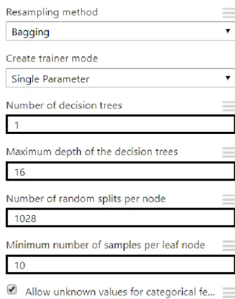
The third validation test is tuned with the following parameters from figure 10:

(28)

22

The overall accuracy for these parameters yields in 99.49%.

The validation tests show that the third test yields the highest accuracy (99.49%), therefor the following parameter combination are chosen for the multiclass decision forest.

 Resampling method: Bagging

 Create trainer mode: Single parameter  Number of decision trees: 100

 Maximum depth of the decision trees: 32  Number of random splits per node: 128  Minimum number of samples per leaf node: 10

 Allow unknown values for categorical features: check 5.2.1.2 Multiclass Neural Network

The multiclass neural network algorithm is validated with three different combination of parameters.

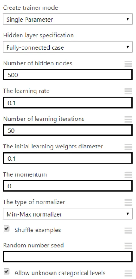
The first validation test is tuned with the following parameters (default in azure) from figure 11:

Figure 11: Hyper-parameters for the Multiclass Neural Network algorithm The overall accuracy for these parameters yields in 97.33%.

(29)

23

(30)

24

The validation tests show that the first test yields the highest accuracy (97.33%), therefor the following parameter combination are chosen for the multiclass neural network.

 Hidden layer specification: Fully-Connected case  Number of hidden nodes: 100

 The learning rate: 0.1

 Number of learning iterations: 100

The maximum number of time the network should iterate through the input data.  The initial learning weights diameter: 0.1

 The momentum: 0  The type of normalizer:  Shuffle examples: check

 Allow unknown categorical levels: check 5.2.1.3 Multiclass Decision Jungle

The multiclass decision jungle algorithm is validated with three different combination of parameters.

(31)

25

The first validation test is tuned with the following parameters from figure 14:

Figure 14: Hyper-parameters for the Multiclass Decision Jungle algorithm The overall accuracy for these parameters yields in 94.13%.

(32)

26

The validation tests show that the second test yields the highest accuracy (98.56%), therefor the following parameter combination are chosen for the multiclass decision forest.

 Hidden layer specification: Fully-Connected case  Number of hidden nodes: 100

 The learning rate: 0.1

 Number of learning iterations: 100  The initial learning weights diameter: 0.1  The momentum: 0.1

Selects the method for normalization of the input data’s features.  Shuffle examples: check

 Allow unknown categorical levels: check

5.2.2 Data pre-processing

Before the input data is used to build the machine learning model, some properties and

arrangement of the input dataset should be processed. After all, the most important key point of a machine learning project is the dataset (Chicco, 2017). Data processing involves feature extraction (normally done in the data collection), cleaning the dataset from missing rows and noise, filtering or normalization, feature selection (selecting only relevant features) and other statistic techniques that helps the algorithm to be effectively trained.

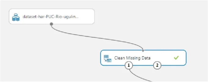
First, both data sets are cleaned from missing values. Azure provides a module which performs this, it can be seen in figure 17 as “Clean Missing Data”. It is configured to remove entire rows where data is missing, on all columns.

(33)

27

Figure 17: Data set and Clean Missing Data module in Azure Machine Learning Studio

After the dataset has been processed, the module outputs the cleaned data set. For both the Ugolino data set and the two Android sets, no data is missing so the data sets remain the same as before, with the same number of attributes and columns.

After cleaning, filter-based feature selection is performed to filter out irrelevant attributes in the data set. This is an important tool in machine learning to help identify columns that has the most predictive power to desired output. Azure machine learning supports Pearson correlation statistic, after providing a data set and specifying the label column, it returns a ranking score for the correlation of each feature, see ranking of Ugolino’s data set in table 7.

Table 7: Ugolino data set attributes

Feature selection process shows that how tall_in_meters and body_mass_index in the Ugolino data set has a high correlation to each other, therefor the column body_mass_index is removed. It also scores 0 for the attribute user, meaning it does not contain any valuable information for the model, thus it also removed.

In the two Android data sets, there is only four numerical values, x, y, z and time. The column activity is the target label, but the sensor column is a string and is therefore defined as a

category (when defining a category in Azure ML studio, the attribute remains in the data set but are not processed). The time column contains a timestamp for each sample, but because the time was not related to the activity when data collection was done, it is also removed. See table 8.

User Gen_der Age How _tall_ in_m eter s Wei ght Bod y_m ass_i ndex X1 Y1 Z1 X2 Y2 Z2 X3 Y3 Z3 X4 Y4 Z4 class 0 0 0.08₄₆₄ 0.02410 3 0.02 133 9 0.02 222 9 0,12 839 9 0.62 738 1 0.74 189 1 0.39 396 2 0.37 669 8 0.44 935 0.10415 0,39 451 5 0,10 415 4 0,63 302 4 0,61 522 8 0,49 284 5 1

(34)

28 Table 8: Android data set attributes

sensor x y z time activity

string double double double long string

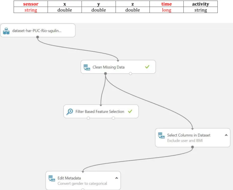
The attributes are removed through a module called Select Columns in Dataset, which allows for excluding columns in a data set. Additionally, the feature gender from the Ugolino data set is defined as categorical, because it contains a string value which cannot be processed in the algorithms training. Edit Metadata module is used to define categories. See figure 18.

5.2.3 Evaluation methods and measures

Evaluating the machine learning model is an essential step, it is the key to verify how well the model performs and a way to compare it against others. 10-fold cross validation is used to evaluate the classifier built in this paper, on all three different algorithms, with three different data sets. The technique is useful because it splits and randomizes the training data and the test data, and then iterates and shifting them 10 times. This helps to avoid underfitting and

overfitting. More test data is used because the entire data set is used for both training and evaluation, compared to the hold-out technique for example, which only tests the data from a single partition. However, 10-fold cross validation is thus much more computationally intensive. The technique generates 10 different folds, with evenly distributed number of samples in each Figure 18: Overview over the data pre-processing modules in Azure Machine Learning Studio in Ugolino data set

(35)

29

fold. Performance statistics are returned for each fold, but also a mean value from all folds together. The mean value is used in this paper to compare the result.

The 10-fold cross validation technique outputs several metrics for each class. Accuracy, recall, precision and f-measure is used in this paper to evaluate and compare the results.

Accuracy is good to get a quick overall view of the classifiers performance, it measures the number of correct predictions made divided by the total number of predictions, and it is represented as a percentage where 100% means that all predictions are correct. Accuracy is calculated manually through the formula (1) in chapter 2.1.3.

It’s good however to look at more detailed metrics such as recall and precision to get a more truthful evaluation. Recall is for example important to observe when dealing with an imbalanced dataset. An imbalanced dataset means that one or more classes in the dataset contains the majority of all the samples, they are not equally represented. This can lead to that the algorithms generalizes the predictions to the majority classes, because more training has been done with them. For example, in a binary classification model, if a class A contains 97% of all the instances in the training data set, and the other class B, contains only 3%. This would generate an overall accuracy of 97%, which seems quite good, but it might be that the model only correctly classifies class A and misclassifying all the instances in class B (Han, et al., 2012). Recall would reveal this phenomenon, if it has a low score (the highest score is 1.0).

Precision is used to look at how precise the model predicts. Which means that every instance that has been classified as class A, actually are class A (1.0 is the highest score). But it doesn’t tell how many instances that were missed. Whereas recall tells how many instances of a class that were classified as such, but it does not tell how many of them are wrong.

Azure machine learning studio produces accuracy, recall and precision automatically when using the built-in 10-fold cross validation technique. F-measure is calculated manually (in the Azure model) using the formula (4) from chapter 2.1.3. Accuracy, precision, recall and f-measure is round off to 3 decimals.

In addition to this, the studio generates a confusion matrix such as the one in table 9, although table 9 is manually created. The boxes show the percental number of TP and error for each class, the TP is the blue-filled diagonal boxes. For example, the box in the actual class A, and the

predicted class A, a TP percentage of 90% can be observed, this means that 90% of all the instances in class A, are predicted as such. It’s important to mention that the score in the confusion metrics is rounded off, to one decimal. If the box does not contain any value such as the box between actual class B and predicted class D, this is equal to zero instances. If a box scores 0.0%, this mean that some instances were classified, but too few to be shown after rounding.

(36)

30

Table 9: Azure confusion matrix showing the percentage outcome for five classes

Predicted Class

ClassA ClassB

ClassC

ClassD

ClassE

A

ct

u

al

Cl

ass

ClassA

90.0%

0.0%

ClassB

0.1%

57.1%

0.2%

0.1%

ClassC

0.0%

99.9%

0.0%

ClassD

0.1%

2.8%

0.2%

96.2%

0.7%

ClassE

0.0%

0.1%

99.8%

A weighted average is also calculated when the average for precision, recall and F-measure is calculated. A weighted average is calculated in same way as the average, but all the values are weighted depending on the frequency of occurrence for each class. A class with a higher frequency of occurrence is given a lower weight.

5.3 E

VALUATION RESULT

First, the performance results from the Ugolino paper are presented, the machine learning model is trained and evaluated with the data set collected in the same paper.

Secondly, the performance result of the machine learning model built in this paper, consisting of the three different algorithms, are evaluated. Trained and evaluated by the data set collected in the Ugolino paper.

Lastly, this papers machine learning model’s performance result is presented, when being trained and evaluated with the data collected through the Android device built in this paper. In the end a comparison chart between the results is presented.

5.3.1 Ugolino machine learning model

In this chapter the performance metrics for the machine learning model in Ugolino’s, paper is shown, where the C4.5 decision tree in combination with AdaBoost ensemble method is used. 10-fold cross validation is used to evaluate the model and accuracy, precision, recall and f-measure is available.

(37)

31 In table 10 the confusion matrix can be observed.

Table 10: Confusion Matrix from Ugolino's machine learning model Predicted Class

Actual class Sitting Sitting down Standing Standing up Walking

Sitting 50 601 9 0 20 1

Sitting down 10 11 484 29 297 7

Standing 0 4 47 342 11 13

Standing up 14 351 24 11 940 85

Walking 0 8 27 60 43 295

Table 11 shows the precision, recall and f-measure for each class.

Table 11: Precision, recall and f-measure per class from Ugolino’s machine learning algorithm

PRECISION RECALL F-MEASURE CLASS

1,000 0,999 0,999 Sitting 0,969 0,971 0,970 Sitting down 0,998 0,999 0,999 Standing 0,969 0,962 0,965 Standing up 0,998 0,998 0,998 Walking 0,994 0,994 0,994 Weighted Avg.

(38)

32

Table 12 shows the percental outcomes of TP, FP, TN and FN for each class.

Table 12: Visualized Confusion Matrix showing the models percental outcome of each class in the Ugolino’s data set Predicted Class Sitting Sitting Down Standing Standing Up Walking Ac tu al C la ss Sitting 99.9% 0.0% 0.0% 0.0% 0.0% Sitting Down 0.1% 97.1% 0.2% 2.5% 0.1% Standing 0.0% 0.0% 99.9% 0.0% 0.0% Standing Up 0.1% 2.8% 0.2% 96.2% 0.7% Walking 0.0% 0.0% 0.1% 0.1% 99.8%

Table 13 shows the machine learning models overall accuracy for all predicted instances from the Ugolino’s dataset.

Table 13: Overall accuracy of all instances from Ugolino´s data set

Correctly Classified Instances 164662 99.4144 %

Incorrectly Classified Instances 970 0.5856 %

5.3.1.1 Analysis

It can be found that the total correctly classified instances (TP) are 164 662, yielding in a 99.4144% accuracy. The number of incorrectly classified instances are 970, equal to 0.5856%. As can be seen by the table 12, the classes sitting and standing scores the highest number of TP, along with walking. Walking however, has a lower recall as can be seen in table 11. Sitting has a precision equal to one, recall measure at 0,999, F-Measure 0,999, thus sitting is the activity with overall highest performance.

Sitting down and standing up are the classes with the lowest precision rate, as well as the lowest F-measure. It can also be observed here that recall is lower than the other classes. At the bottom of table 11, the average of each class can be seen.

A possible explanation to some of these results can be because of the different amount of collected samples the classes has. Sitting and standing for example, which has the highest score, has the highest number of samples. Sitting down and standing up which has the lowest results,