School of Education, Culture and Communication
Division of Applied Mathematics
BACHELOR THESIS IN MATHEMATICS / APPLIED MATHEMATICS
American Option pricing under Multiscale model using Monte Carlo and
Least-square approach
by
Tiffany Bart Adde
Kadek Maya Sri Puspita
Kandidatarbete i matematik / tillämpad matematik
DIVISION OF APPLIED MATHEMATICS
MÄLARDALEN UNIVERSITYSchool of Education, Culture and Communication
Division of Applied Mathematics
Bachelor thesis in mathematics / applied mathematics
Current version:
19th June 2017
Project name:
American Option pricing under Multiscale model using Monte Carlo and Least-square ap-proach
Authors:
Tiffany Bart Adde and Kadek Maya Sri Puspita
Supervisor: Jan Röman Co-supervisor: Linus Carlsson Reviewer: Richard Bonner Examiner: Anatoliy Malyarenko Comprising: 15 ECTS credits
Abstract
In the finance world, option pricing techniques have become an appealing topic among re-searchers, especially for pricing American options. Valuing this option involves more factors than pricing the European style one, which makes it more computationally challenging. This is mainly because the holder of American options has the right to exercise at any time up to maturity. There are several approaches that have been proved to be efficient and applicable for maximizing the price of this type of options. A common approach is the Least squares method proposed by Longstaff and Schwartz. The purpose of this thesis is to discuss and analyze the implementation of this approach under the Multiscale Stochastic Volatility model. Since most financial markets show randomly variety of volatility, pricing the option under this model is considered necessary. A numerical study is performed to present that the Least-squares ap-proach is indeed effective and accurate for pricing American options.
Acknowledgments
We would like to express our gratitudes to our supervisors, Linus Carlsson and Jan Röman for their patience, guidance and motivation. Their input truly helped us through our time of research and writing of this thesis. We would also like to thank our examiner Anatoliy Malyarenko for his informative feedback.
Contents
Introduction 1 1.1 Literature review . . . 1 1.2 Research question . . . 2 1.3 Methodology . . . 2 Derivative Pricing 3 2.1 American options . . . 32.2 The Binomial tree . . . 3
2.3 Black and Scholes model . . . 5
2.4 Monte Carlo methods . . . 6
2.5 Least-Squares approach . . . 7
2.5.1 Numerical example for the Least-Square approach . . . 8
American option pricing under Multiscale model using Monte Carlo methods 13 3.1 Multiscale Stochastic Volatility model . . . 13
3.2 Simulation of Multiscale Stochastic Volatility model . . . 14
Results 16 4.1 A Numerical Implementation of LSM . . . 16
4.2 A Numerical Example of Monte Carlo simulation under Multiscale Volatility Model . . . 17
4.3 A Numerical Example of Monte Carlo simulation and Least-Square Approach under Multiscale Volatility Model . . . 21
Conclusion 23
List of Figures
2.1 Binomial Tree . . . 5 4.2 The figure shows a fast mean-reverting stochastic process. We see that the
process goes from about 0.25 up to 0.55, which is proven to be the fast one, or in other words, the movements of the volatility are very extreme. This being compare to a slow mean-reverting process. The thicker line symbolizes the mean result for all simulations. . . 18 4.3 The figure shows the stock price under the fast mean-reverting process. The
graph shows that, indeed, the prices are more concentrated to one point than the one in Figure 4.5. The thicker line symbolizes the mean result for all simulations. . . 18 4.4 The figure shows a slow mean-reverting process. We can see that compare to
the V1from Figure 4.2 the difference between the highest value and the lowest
is much lower as it only goes from 0.37 to 0.44. This stochastic process has less drastic changes than V2. The thicker line symbolizes the mean result for
all simulations. . . 19 4.5 This figure is the graph of stock price under slow mean-reverting process.
Compared to the MSVM with the fast mean-reverting process, this figure shows less concentrated paths. The thicker line symbolizes the mean result for all simulations. . . 19 4.6 The figure shows both slow and fast mean-reverting processes using Monte
Carlo simulation. The thicker line symbolizes the mean result for all simulations. 20 4.7 The figure shows the stock price under both fast and slow mean-reverting
pro-cesses. This shows less concentrated paths than the fast mean-reverting (see Figure 4.3), however more than the slow mean-reverting one (see Figure 4.5). The thicker line symbolizes the mean result for all simulations. . . 20
List of Tables
2.1 Stock price . . . 9
2.2 Value of the American put option at t = 3 . . . 9
2.3 Early exercise decision at t = 2 . . . 11
2.4 Cash flow of the American put option at t = 3 . . . 11
2.5 Early exercise decision at t = 1 . . . 12
2.6 Cash flow . . . 12
4.7 Results of Numerical example for American Put option . . . 16
4.8 Results of Numerical example for American Call option . . . 17
4.9 Results for American Put option with MSVM under LSM . . . 21
Introduction
Determining the price of American style options, with the ability to exercise early, has been a major task in derivatives finance. The chances are big that these type of derivatives can be found in all financial markets, including, equity, foreign exchange, agriculture, insurance, etc. The classical model, the binomial options pricing model, is commonly used due to its simpli-city and applicability to handle a variety of conditions compare to other models. The method of this model is by creating a graph that resembles a tree, which is often called the binomial tree. The model traces the evolution of the option’s important underlying variables in discrete time. The drawback is that this model becomes less practical in option pricing that involves multiple factors. Based on this reason, several numerical techniques have been developed over the years, for instance, the Least-square Monte Carlo approach introduced by Longstaff and Schwartz [14]. In order to obtain the optimal exercise strategy that maximizes the payoff, the simulation methods solve the problem given the stochastic nature of the underlying stock price. Although computationally time-consuming, the Monte Carlo simulation can converge to the solution faster for higher number of simulations.
In recent years, several researchers have considered using the stochastic volatility model to approximate the price of an option. The models are developed to eliminate the assumption of constant volatility by the Black-Scholes model [2]. Over the life of the derivative, the underlying volatility does get affected by the changes in the price level of the underlying security. By allowing the price to differ, this improves the accuracy for the calculations of this model. In this thesis, we consider a multiscale stochastic volatility model studied in [4]. This model consists of three stochastic variables and volatilities which modulated by changes occurring on fast or slow time scales.
1.1
Literature review
The use of Monte Carlo simulation for pricing American option is first attempted by Tilley [16]. His approach uses the backward algorithm and bundling technique which apply to the valuation of a single asset American put option. Even though he accomplished to show that there exists a useful algorithm for valuing American option in a path simulation, another prob-lem arose when pricing an option which was based on several underlying assets. To address this problem, Broadie and Glasserman [3] developed a method which generates two estimat-ors that converge to the true price. However, their estimatestimat-ors are limited under two decisions only, exercise or not exercise the option. Based on the early exercise features in American options, Longstaff and Schwatz in [14] developed a practical Monte Carlo method by
apply-ing the least-squares regression on polynomials. They estimate the continuation values of the underlying assets and using only in-the-money path in the regression to increase the capability. The existence of a skew or the smile curve of the option’s implied volatility has been proven to be true in many studies. By applying the stochastic volatility models proposed by researchers, for example [10], [12], one can capture the movements of the volatility. In [8], Christoffersen et al. show the purpose of using two stochastic volatilities model is that one could capture the random movements on the asset prices and the random behaviour of market risks better, unlike using only one stochastic volatility. Chiarella and Ziveyi in [5] presented a numerical integration technique for pricing an American call option under two-factor stochastic volatilities of mean reversion type. By applying the Fourier and Laplace transforms, they are able to present an approximate formula for pricing American option. They also analyzed the effects of varying the volatilities of instantaneous variance on both the early exercise boundary and the corresponding option prices. For an overview of the recent developments in the use of multiscale volatility model for pricing American option, Agarwal et al. [1] use perturbative expansion techniques to approximate the price of a single asset put and the optimal exercise boundary. In their paper, they also stated that the fast and slow-scale approximations are equally accurate if the scaling parameter value is equal to unity. Canhanga et al. in [4] uses similar model studied in [5] for valuing European options. They analyzed the applicability and similarity between the three different methods, the asymptotic expansion method, Fourier and Laplace, and Monte Carlo simulation in order to find the true value of European options.
1.2
Research question
In this thesis, we study the application of appropriate models for pricing American options. By analyzing the performance of this models and then comparing the pricing results, we answer the following questions: How applicable the Multiscale Stochastic Volatility model is in pro-gramming and how to value the American options under this model using the Least-squares Monte Carlo approach.
1.3
Methodology
In order to implement this research, the models applied are the binomial pricing model and the Least-square Monte Carlo under the Multiscale Stochastic Volatility model. We use the price from the binomial as our reference price. Then by collecting other important parameters, including, the initial asset price, strike price, time to maturity, etc., we begin our simulation which is performed throughout in Python 3.6.
The thesis is organized in the following structure: An introduction to the important features of American options and theoretical specifications of the various option pricing models are given in the next section. Section 3 contains a brief introduction of the Multiscale Stochastic model for pricing American put options. The result of the simulation and comparison of the models is presented in Section 4. Finally, the conclusion is provided in the last section.
Derivative Pricing
2.1
American options
An option is a contract that gives the holder the right but not the obligation to buy (call) or sell (put) the security or asset. The most common traded options are European and American op-tions. In contrast with European option, an American option is an option that can be exercised at any time, before or at the maturity date. Due to its ability to exercise early, pricing Amer-ican options is considered challenging by researcher according to Longstaff and Schwartz in [14]. As oppose to a call option, a put option is considered in the money when S < K, at the money when S = K and out of the money when S > K, where S is the stock price and K is the strike price. If the option is out-of-the-money at time t, then it is better not to exercise. However, if the option is in-the-money, the holder has to consider whether or not they want to wait to exercise the option since the payoff might be even bigger in the future. Alternatively, exercise the option and lose this opportunity. The payoff of American option can be calculated by using the following formulas:
C(0,t) = 0 for all t∈ [0, T ] and C(S, T ) = max{S − K, 0},
P(∞,t) = 0 and P(S, T ) = max{K − S, 0},
where T is the maturity date, C denotes the call price and P the put price. According to Hull in [11], the value of American and European calls are the same under no dividends. However, American put is worth more than European put options.
2.2
The Binomial tree
In order to find the value of an American option the most common used model is the Binomial tree. The binomial options pricing model which originates from the Black-Scholes-Merton model is introduced by Cox, Ross and Rubinstein in 1979, see [7]. This model is considered as one of the easiest ways for pricing American options. This technique constructs a diagram showing different possible intrinsic values that an option may follow at different nodes or time periods. One way of valuing the American option involves a backward algorithm which re-quires us to work from the maturity date to the starting point of the option’s life. It is important to check at each node whether exercise the option early is optimal or not. At each node, the
value of the option depends on the probability of increasing or decreasing the underlying asset by a certain percentage amount. Let us imagine that we have a stock price at time 0, where there is a certain probability that option can go up or down which can be calculated by using the formula bellow
u= eσ √ ∆t, d= e−σ √ ∆t, p=e r∆t− d u− d ,
where σ is the volatility, ∆t is the length of the time step on a binomial tree, u and d are the parameters of up and down movements and p is the probability under the risk-neutral world measure.
There can be many time steps which is indicated by the length of the time steps ∆t. For example if there is two up movements the value of the option will be denoted by fuu, one up
and one down movement by fud and two down movement by fdd. The value of the option of
one step binomial tree is calculated as follows
f = e−r∆t[p fu+ (1 − p) fd]. (2.1)
If more time steps come in consideration we repeat the Equation (2.1) and get for a two movements binomial tree
fu= e−r∆t[p fuu+ (1 − p) fud], (2.2)
fd= e−r∆t[p fud+ (1 − p) fdd], (2.3)
f = e−r∆t[p fu+ (1 − p) fd]. (2.4)
In order to calculate the real value of the option we substitute Equations (2.2) and (2.3) in (2.4) and get
f = e−2r∆t[p2fuu+ 2p(1 − p) fud+ (1 − p)2fdd]. Figure 2.1 shows how the Binomial Tree looks like.
S0 f S0d fd S0u fu S0d2 fdd S0ud fud S0u2 fuu (1 −p) p p2 (1 − p)p (1 −p)p (1 −p)2
Figure 2.1: Binomial Tree
2.3
Black and Scholes model
Black-Scholes is the primary pricing model that are widely used to calculate the fair price of option, based on six variables such as volatility, type of option, underlying stock price, time, strike price, and risk-free rate.
This model is effectively used to determine the price of a European option, which is an option that must be held to maturity. For pricing the European option with no dividend, the Black-Scholes-Merton(1973) formula is given by:
C(S, t) = SN(d1) − Ke−r(T −t)N(d2),
P(S, t) = Ke−r(T −t)N(−d2) − SN(−d1),
where N(.) is the cumulative distribution, (T − t) is time to maturity and d1, d2are given by
d1= ln(S/K) + (r + σ2/2)(T − t) σ √ T− t , d2= ln(S/K) + (r − σ 2/2)(T − t) σ √ T− t ,
which can also be written as
d2= d1− σ
√ T− t.
The Black-Scholes formula is not suitable for pricing American option because it relies on the assumption that there exist only one predetermined maturity date.
2.4
Monte Carlo methods
In mathematical finance, the Monte Carlo simulation is introduced by Boyle in 1977. Monte Carlo becomes attractive for valuing complex financial derivatives which helps to evaluate high-dimensional integrals. This can be shown by using the Monte Carlo method to estimate the value of an integral f , mathematically it can be written as [9]:
α =
Z 1
0
f(x)dx.
We factorized the function f (x), then the expected value is given by
α = E[a(x)] =
Z 1
0
a(x)ρ(x)dx.
From the density ρ(x), we generate an i.i.d sample x1, x2, . . . , xn to estimate the expected
value as ˆ α = 1 n n
∑
i=1 a(xi),where n is the number of random points. By the law of large numbers, suppose that a(x) is integrable, then
ˆ
α −→ α almost surely as n −→ ∞. However, if a(x) is also square-integrable, we define
σ2= Var[a(x)] = Z 1 0 (a(x) − α) 2 ρ (x)dx, which gives √ n( ˆα − α ) σ −→N (0,1).
This means that the error ˆα − α in the Monte Carlo estimate is normally distributed with mean 0 and standard deviation σ2/√n, which gives the convergence1 rateO(n−1/2). This shows that the methods have a slow convergence but do not change as the dimension increases. Based on this reason, the Monte Carlo methods are not very attractive in evaluating integrals in one dimension, but as dimensions increase so do their attractiveness.
In general, Monte Carlo method works well for valuing European options. The method shows the evolution of underlying asset prices, interest rate and other important factors of the security by simulating as many sample paths as desired under the stochastic processes. Pricing the European options is determined only by the stock price at a given starting point, maturity time, constant interest rate and volatility. However, pricing American options also require the information of option value at the intermediate times between the simulation start time and
1Here, the convergence means that the Monte Carlo simulations will never give an exact answer, but
the option maturity time which in this method is harder to obtain. Since pricing this option involves backward algorithm, the Monte Carlo methods become computationally complex.
To achieve a more accurate approximation of valuing complicated path-dependent option, where it is necessary to divide a time interval [0, T ] into subintervals, we have the following illustration. Assume that the stock price grows in time according to a stochastic differential equation given bellow
dS(t) = µ S(t)dt + σ S(t)dW (t), (2.5) with µ a risk-free rate and W (t) a standard Brownian motion that follows the properties [15]: • W (0) = 0.
• If r ≤ s ≤ t ≤ u, W has independent increments, which means that W (u) −W (t) and W (s) − W(r) is independent.
• W (t) −W (s) is normally distributed with mean 0 and variance√t− s, N(0,√t− s).
• W (t) has continuous paths which can be proven by using the Kolmogorov’s continuity the-orem, see [17].
Generalizing the Equation (2.5), gives the following dynamics
dS(t) = µS(t)dt + σ (S(t))S(t)dW (t). (2.6)
This equation shows that σ is dependant on the stock price S(t), as explained in [9]. The approximation of Equation (2.6) gives us the following
S(t + ∆t) = S(t) + µS(t)∆t + σ (S(t))S(t)W (t),
where ∆t = T /n, since we consider n to be the number of time steps. The Wiener process W(T ) is distributed as√∆tZ where Z is a standard normal random variable. The process then can be simulated by the following equation
S(t + ∆t) = S(t) + µS(t)∆t + σ (S(t))S(t)√∆tZ.
2.5
Least-Squares approach
The Least Squares Monte Carlo (LSM) approach, which is developed by Longstaff and Schwartz, see [14] , is popularly used to deal with the problems of pricing American options mentioned above. Their approach uses least-squares analysis to find the optimal option price by compar-ing the value of continuation with the immediate exercise value at each time an early exercise has to be made. This involves regressing the discounted future cash flows found from continu-ation on a finite set of functions in the underlying stock prices. In other words, the intention of the Least-Squares method is to find paths of approximation that find the optimal exercising point in order to maximize the value of the American option.
Assuming an American option is alive within the time horizon [0, T ]. Within the time horizon, early exercise can only be done at the J discrete times 0 < t1≤ t2≤ ... ≤ tj= T . At
exercise time tk, if the payoff of immediate exercise is positive and higher than the value of continuation, that option should be exercised immediately. This continuation value is the re-maining value of the option that cannot be exercised until after tk, which can also be expressed
as conditional expectation of the option payoff under the risk-neutral pricing measure Q.2 The following algorithm is based on the Longstaff and Schwartz approach. Introducing the notation Ctj as the cashflow vector at the last timestep tj. We determine the cashflow, which
is the payoff of a call option, in other words, has zero continuation value, of each simulation i by the following formula:
Ci, tj = max(Si, tj− K, 0).
We then estimate the exercise value by selecting the stock prices at time-step tj−1, which
has the following condition
max(Si, tj−1− K, 0) > 0.
By regressing the discounted future cash-flows realized from continuing onto a finite set of basis function of our stock price, we can then obtain the continuation value for path i with values Si, tn at time tn[14]: Fi, tn−1 = ∞
∑
j=0 aj(tn) Lj(S),where aj are constant coefficients and Lj is the set of basis functions. The regression is
per-formed by using all the values from all of the paths with the basic function of any degrees polynomial. We can then exercise the American option at an early stage when it fulfills the condition bellow
Ci, tn−1 > Fi, tn−1.
Further, by working backward, we obtain the early exercise at each time-step. This lets us to build the value matrix from the cash flow vectors Ci, tn, by concatenating the cashflow
vectors Ci, tn, where n = 1, · · · , J. The option value is then decided by discounting each cash
flow back to the starting point and calculating the mean of the results.
2.5.1
Numerical example for the Least-Square approach
Longtstaff and Schwartz presented in their paper [14] a simple numerical example in order to understand the Least-Square method. This is considered a simple numerical example as there only is 8 paths when the number of paths should be higher to resemble reality. Using the same example as in [14], in this section we are going to mathematically show an in-depth explanation of the approach.
2Q measure is a probability measure which is derived from the assumption that the present value of the
Let us assume that we have the collected data as shown in Table 2.1. We consider an Amer-ican put option where the strike price is 1.10 and the risk-free rate is 6% with no-dividend.
Table 2.1: Stock price
Path t = 0 t= 1 t= 2 t= 3 1 1.00 1.09 1.08 1.34 2 1.00 1.16 1.26 1.54 3 1.00 1.22 1.07 1.03 4 1.00 .93 .97 .92 5 1.00 1.11 1.56 1.52 6 1.00 .76 .77 .90 7 1.00 .92 .84 1.01 8 1.00 .88 1.22 1.34
From Table 2.1, we focus on the stock price at t = 2 and collect the stock prices that are in-the-money which means K − St > 0. In other words, the "in-the-money" stock prices, denoted
as S, are 1.08, 1.07, .97, .77, and .84, which lay on paths 1, 3, 4, 6 and 7. At time t = 3, we would then have the value for these paths as shown in Table 2.2.
Table 2.2: Value of the American put option at t = 3
Path max(0, K − S3) 1 .00 3 .07 4 .18 6 .20 7 .09
The values of the option in t = 2 are 0.00e−0.06 ·1, 0.07e−0.06 ·1, 0.18e−0.06 ·1, 0.20e−0.06 ·1, 0.09e−0.06 ·1 which we denote as V . We now assume that for these paths, we have an approx-imation in the following form
V = a + bS + cS2,
where a, b, c are constants. In order to find these constants, we have to find the minimum error for all the five paths.
min a,b,c 5
∑
i=1 (Vi− a − bSi− cS21)2. (2.7)We denote Equation (2.7) as f (a, b, c). To find the minimum error, we ought to differentiate the function f with respect to a, b, c and equal it to 0.
∂ f ∂ a = −2 5
∑
i=1 (Vi− a − bSi− cS21) = 0, ∂ f ∂ b = −2 5∑
i=1 Si(Vi− a − bSi− cS21) = 0, ∂ f ∂ c = −2 5∑
i=1 S2i(Vi− a − bSi− cS21) = 0.This leads to the following system of linear equations
5a + b 5
∑
i=1 Si+ c 5∑
i=1 S2i = 5∑
i=1 Vi, a 5∑
i=1 Si+ b 5∑
i=1 S2i + c 5∑
i=1 S3i = 5∑
i=1 ViSi, a 5∑
i=1 Si2+ b 5∑
i=1 S3i + c 5∑
i=1 S4i = 5∑
i=1 ViS2i.Given the following matrix rules
A a b c = B, where A is 5 ∑5i=1Si ∑5i=1S2i ∑5i=1Si ∑5i=1S2i ∑5i=1S3i ∑5i=1S2i ∑ 5 i=1S3i ∑ 5 i=1S4i , and B is ∑5i=1Vi ∑5i=1ViSi ∑5i=1ViS2i . This gives us 5 ∑5i=1Si ∑5i=1S2i
∑5i=1Si ∑5i=1S2i ∑5i=1S3i ∑5i=1S2i ∑ 5 i=1S3i ∑ 5 i=1S4i a b c = ∑5i=1Vi ∑5i=1ViSi ∑5i=1ViS2i .
Data from Table 2.1 has the solution a = −1.070, b = 2.983 and c = −1.813 and our equation for the value became3
3The code used to solve this can be found in Mathews, J. H., & Fink, K. D. (2005). Numerical methods using
V = −1.070 + 2.983S − 1.813S2.
Hence, we get the cash flow of continuing and exercising at t = 2 as shown in Table 2.3. (OTM=out of the money).
Table 2.3: Early exercise decision at t = 2
Path Exercise: K − S(t2) Continuation: V (S(t2))
1 .02 .0369 2 OTM OTM 3 .03 .0461 4 .13 .1176 5 OTM OTM 6 .33 .1520 7 .26 .1565 8 OTM OTM
From Table 2.3, we can see that for the paths 4, 6 and 7 early exercise values are bigger than the values of continuing. Therefore, we decide to exercise at those points. Then the cash flow for t = 3 are shown in Table 2.4. Observe that the cash flow is 0 when the option is exercised on the previous time steps.
Table 2.4: Cash flow of the American put option at t = 3
Path max(0, K − S3) 1 .00 2 .00 3 .07 4 .00 5 .00 6 .00 7 .00 8 .00
Now we look at Table 2.1, where t = 1. We see that the paths 1, 4, 6, 7 and 8 are in the money. As for t = 2, we found the equation of the value for continuing by using the same formula as Equation (2.7). We get
V = 2.038 − 3.335S + 1.356S2.
Table 2.5 shows that the values of decision for the early exercise and the values of con-tinuing when t = 1. We see that the exercise values at paths 4, 6, 7 and 8 are higher than the
continuing, hence, we decide to early exercise. We show the cash flow for t = 1, t = 2 and t = 3 in Table 2.6.
Table 2.5: Early exercise decision at t = 1
Path Exercise: K − S(t1) Continuation: V (S(t1))
1 .01 .0139 2 OTM OTM 3 OTM OTM 4 .17 .1092 5 OTM OTM 6 .34 .2866 7 .18 .1175 8 .22 .1533
Table 2.6: Cash flow
Path t = 1 t= 2 t= 3 1 0 0 0 2 0 0 0 3 0 0 .07 4 .17 0 0 5 0 0 0 6 .34 0 0 7 .18 0 0 8 .22 0 0
The value of the option become
0.07e−0.06·3+ 0.17e−0.06·1+ 0.34e−0.06·1+ 0.18e−0.06·1+ 0.22e−0.06·1
8 = 0.1144. (2.8)
Equation (2.8) says that the value of the option under LSM is 0.1144, which is higher than K− S(t0) = 1.1 − 1 = 0.1, hence it is not optimal to exercise early.
American option pricing under Multiscale
model using Monte Carlo methods
3.1
Multiscale Stochastic Volatility model
The Multiscale Stochastic Volatility model (MSVM) approaches a linear approximation that has a component of the well-known Black-Scholes SDE. As opposed to the Black-Scholes formula, the MSVM does not assume that there is a constant volatility. It has also been proven that a single volatility does not fit the real world observed financial data. Indeed, this model contains two correlated volatilities, one moving fast and the other moving slow. In the finance world, the difference between a fast mean-reverting and a slow mean-reverting volatility is significant. With respect to the return of an option, if we assume that a participant has a long position in the case that the volatility is fast mean-reverting, she could then expect that the possibilities to get high return to quickly disappear. Hence, she would try to sell the option in order to keep the high return. On the other hand, if she has a short position, she will most certainly try to keep the option and wait for the price to get lower, therefore, earn a higher profit. If the participant assumes that the mean-reversion is slow, in the case where she is in a long position, she will surely try to keep the option and wait for the price to go up and receive a higher return. In contrast to the long position, when the participant is in a short one she will try to sell the option as fast as possible in order to keep a higher benefit.
We apply the following model as used in [5] and [4]:
dS= µSdt +√V1SdW1+√V2SdW2, (3.9) dV1=1 ε(θ1−V1)dt + r 1 εξ1 √ V1dW3, (3.10) dV2= δ (θ2−V2)dt + √ δ ξ2 √ V2dW4, (3.11)
where µ is the expected return, V1and V2are the variance processes, and ξ1and ξ2 are
con-stants. All the Wiener processes are uncorrelated except dW1together with dW3are correlated
with correlation coefficient ρ13 and dW2 together with dW4 are correlated with correlation
coefficient ρ24. The variance processes V1,V2 are mean reverting processes with reversion
rates of 1ε and δ and long run average of θ1, θ2. The terms
q
1 εξ1and
√
δ ξ2are the so called
We assume, 0 < ε << 1 and 0 < δ << 1, which implies that the process V1 is the fast
mean-reverting and the process V2is slow mean-reverting.
3.2
Simulation of Multiscale Stochastic Volatility model
The problem with the Multiscale Stochastic Volatility model (MSVM) is that it follows a Square-root diffusion. Hence, in order to simulate MSVM we first simplified Equations (3.9), (3.10) and (3.11) by eliminating the slow mean-reverting stochastic process. The equation then become dS= µSdt +√V1SdW1 (3.12) dV1= 1 ε(θ1−V1)dt + r 1 εξ1 √ V1dW3. (3.13)
These has the same parameter as the Heston model [10]
dS(t) = µS(t)dt +pV(t)dW1(t), (3.14)
dV(t) = α(b −V (t))dt + σpV(t)dW2(t), (3.15)
where α is the rate of mean-reverting of the Cox Ingersoll Ross process (CIR) [6], b is the mean value over time , σ is the volatility of the CIR process and W1 and W2 are part of a
two-dimensional Brownian motion. Cox, Ingersoll and Ross proposed a model of interest rate dynamic that is as follows
dr(t) = α(b − r(t))dt + σpr(t)dW (t), (3.16)
where in this case W is a standard one-dimensional Brownian motion. Cox, Ingersoll and Ross suggest that if r(0) > 0 then r(t) will never be negative if 2αb ≥ σ2[9]. An Euler discretization indicate the following simulation
r(ti+1) = r(ti) + α(b − r(ti))∆t + σ
p
r(ti)+√∆tZ
i+1. (3.17)
This being done, we had to assign the correlation between W1and W2. We used a simplified
Cholesky decompositionmethod that says if W1and W2has a correlation of ρ we set W1= z1
and W2= ρz1+
p
1 − ρ2z
2, where z1 and z2are two random variables that are normally
Algorithm 1 The algorithm for the correlation path set W1= Z1 for i = 1, ..., n − 1 do Generating Z1 Generating Z2 term1= ρW1 term2=p1 − ρ2Z 2
W2(i) = term1 + term2 Return W1, W2
end for
Z1and Z2are two brownian motions
Algorithm 2 The algorithm for the volatility path set V (0) = initial volatility
for i = 1, ..., T do Generate Z2
drift = a(µ − V (i − 1))∆t
randomness =pmax(V (i − 1), V (0))√∆tZ2(i − 1)
V(i) = max(V (i − 1), V (0)) + drift + randomness Return√∆tZ2, V
end for
Algorithm 3 The algorithm for the asset price levels set S(0) = initial stock price
for i = 1, ..., T do drift= µ · S(i − 1) · ∆t
vol = CIR(i − 1) · S(i − 1) · HCCP(i − 1) S(i) = S(i − 1) + drift + vol
Return S, CIR end for
where CIR denotes the Cox-Ingersoll-Ross process and HCCP denotes the constructed correl-ated path of Heston model.
Results
In this section, we present the result of some numerical examples by implementing the ap-proaches from the previous sections to price the American options. All the graphs and calcu-lations are performed in Python 3.6. The codes used can be found in Appendix 1.
4.1
A Numerical Implementation of LSM
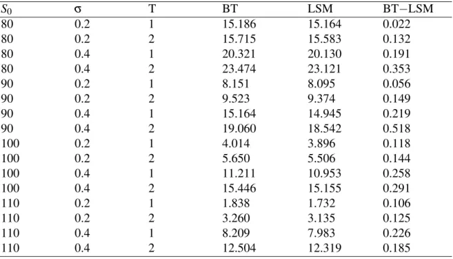
We study and analyze the accuracy of the Least-squares Monte Carlo proposed by Longstaff and Schwartz [14]. The accuracy is controlled by using different parameters and comparing the result from both Binomial Tree (BT) and Least-squares Monte Carlo (LSM) approaches. The fixed parameters used are K = 95, µ = 0.05 and n = 50. The results we got from the BT and LSM with different S0, σ and T are presented in the table below. The number of
simulations we used in LSM was 103and the degree of polynomial is 5.
Table 4.7: Results of Numerical example for American Put option
S0 σ T BT LSM BT−LSM 80 0.2 1 15.186 15.164 0.022 80 0.2 2 15.715 15.583 0.132 80 0.4 1 20.321 20.130 0.191 80 0.4 2 23.474 23.121 0.353 90 0.2 1 8.151 8.095 0.056 90 0.2 2 9.523 9.374 0.149 90 0.4 1 15.164 14.945 0.219 90 0.4 2 19.060 18.542 0.518 100 0.2 1 4.014 3.896 0.118 100 0.2 2 5.650 5.506 0.144 100 0.4 1 11.211 10.953 0.258 100 0.4 2 15.446 15.155 0.291 110 0.2 1 1.838 1.732 0.106 110 0.2 2 3.260 3.135 0.125 110 0.4 1 8.209 7.983 0.226 110 0.4 2 12.504 12.319 0.185
Table 4.8: Results of Numerical example for American Call option S0 σ T BT LSM BT−LSM 80 0.2 1 2.785 2.614 0.171 80 0.2 2 6.631 6.390 0.241 80 0.4 1 8.988 8.713 0.275 80 0.4 2 15.593 15.395 0.198 90 0.2 1 6.973 6.844 0.129 90 0.2 2 12.071 11.629 0.442 90 0.4 1 14.180 13.797 0.383 90 0.4 2 21.745 21.350 0.395 100 0.2 1 13.335 12.967 0.368 100 0.2 2 18.960 18.376 0.584 100 0.4 1 20.448 19.946 0.502 100 0.4 2 28.508 27.870 0.638 110 0.2 1 21.364 20.900 0.464 110 0.2 2 26.933 26.557 0.376 110 0.4 1 27.587 27.297 0.29 110 0.4 2 35.776 35.100 0.676
As we can see from Table 4.7 and Table 4.8, the difference between the price of American options from the two models are minimal. Hence, we assume that the Least-Square Monte Carlo is accurate and we now proceed to apply it to Multiscale Stochastic Volatility model.
4.2
A Numerical Example of Monte Carlo simulation under
Multiscale Volatility Model
In this subsection, we apply and analyze the Monte Carlo simulation into the Multiscale Stochastic Volatility model. The result is achieved by investigating the variance of the fast mean-reverting first, which is denoted by V1. Later on, we apply the same simulation to
in-vestigate the slow mean-reverting, V2. This simulation produce the matrices that will be used
in LSM under multiscale stochastic volatility model to find the optimal price of American put option in Section 4.3. The data we used are µ = 0.06, ε = 0.01, δ = 0.1, θ1= 0.4, θ2= 1,
ξ1= 0.1, ξ2= 1, V10= 0.3 and V20 = 0.3. The number of time steps n was 10 and the number
of simulations m was 100. The small number of simulations was taken in order to see clearer on the graph the results we could get. However, the number of simulations should be higher in order to have a closer result to reality. The results of the simulations can be seen in figures 4.2-4.7.
0 2 4 6 8
Number of time steps
0.30 0.35 0.40 0.45 0.50 0.55
Simulated Asset Price
Heston volatility level with V1
Figure 4.2: The figure shows a fast mean-reverting stochastic process. We see that the process goes from about 0.25 up to 0.55, which is proven to be the fast one, or in other words, the movements of the volatility are very extreme. This being compare to a slow mean-reverting process. The thicker line symbolizes the mean result for all simulations.
0 2 4 6 8
Number of time steps
90100 110 120 130
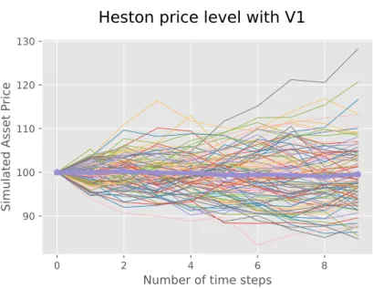
Simulated Asset Price
Heston price level with V1
Figure 4.3: The figure shows the stock price under the fast mean-reverting process. The graph shows that, indeed, the prices are more concentrated to one point than the one in Figure 4.5. The thicker line symbolizes the mean result for all simulations.
0 2 4 6 8
Number of time steps
0.37 0.38 0.39 0.40 0.41 0.42 0.43
Simulated Asset Price
Heston volatility level with V2
Figure 4.4: The figure shows a slow mean-reverting process. We can see that compare to the V1from Figure 4.2 the difference between the highest value and the lowest is much lower as it only goes from 0.37 to 0.44. This stochastic process has less drastic changes than V2. The
thicker line symbolizes the mean result for all simulations.
0 2 4 6 8
Number of time steps
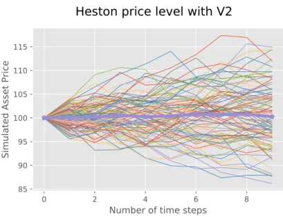
85 90 95 100 105 110 115Simulated Asset Price
Heston price level with V2
Figure 4.5: This figure is the graph of stock price under slow mean-reverting process. Com-pared to the MSVM with the fast mean-reverting process, this figure shows less concentrated paths. The thicker line symbolizes the mean result for all simulations.
0 2 4 6 8
Number of time steps
0.30 0.35 0.40 0.45 0.50 0.55
Simulated Asset Price
MSVM volatility level with v1 & v2
Figure 4.6: The figure shows both slow and fast mean-reverting processes using Monte Carlo simulation. The thicker line symbolizes the mean result for all simulations.
0 2 4 6 8
Number of time steps
8090 100 110 120
Simulated Asset Price
MSVM price level with v1 & v2
Figure 4.7: The figure shows the stock price under both fast and slow mean-reverting pro-cesses. This shows less concentrated paths than the fast mean-reverting (see Figure 4.3), however more than the slow mean-reverting one (see Figure 4.5). The thicker line symbolizes the mean result for all simulations.
4.3
A Numerical Example of Monte Carlo simulation and
Least-Square Approach under Multiscale Volatility Model
This section is to show the Least-Squares approach (LSM) under Multiscale Stochastic Volat-ility model. The degree of polynomial for the LSM is 5. We used the same data as in previous section, however, we used various data for S0, K and m.
Table 4.9: Results for American Put option with MSVM under LSM
m S0 K Value of the option
101 90 90 4.757191 102 90 90 2.908279 103 90 90 2.867147 104 90 90 2.870963 101 90 100 11.687731 102 90 100 10.737611 103 90 100 9.979482 104 90 100 10.204631 101 100 90 0.937536 102 100 90 0.208727 103 100 90 0.411637 104 100 90 0.379972 101 100 100 4.674494 102 100 100 3.188882 103 100 100 3.355485 104 100 100 3.272534 101 100 110 11.269590 102 100 110 10.951877 103 100 110 10.374541 104 100 110 10.218680 101 100 120 25.218587 102 100 120 21.285015 103 100 120 19.812217 104 100 120 19.865982
From Table 4.9, it is seen that the value of the American put options almost always become smaller as the number of simulations increase. We know that it is optimal to exercise when the value of the put option is lower than K − S0[11]. Hence, we can also see when S0= 90, K =
100 and m = 103it is optimal to exercise early since the value of the option is lower than 10. This could also be seen when S0= 100, K = 120 and m = 103, 104.
Table 4.10: Results for American Call option with MSVM under LSM
m S0 K Value of the option
101 90 80 12.536949 102 90 80 10.520097 103 90 80 10.386099 104 90 80 10.111837 101 90 90 4.258010 102 90 90 4.324485 103 90 90 3.210943 104 90 90 2.999685 101 90 100 1.930878 102 90 100 0.740802 103 90 100 0.414090 104 90 100 0.457204 101 100 90 14.807385 102 100 90 10.412125 103 100 90 10.088410 104 100 90 10.310712 101 100 100 4.373181 102 100 100 3.498181 103 100 100 3.501646 104 100 100 3.459526 101 100 110 1.320540 102 100 110 0.496555 103 100 110 0.708829 104 100 110 0.632238
We also try to implement the approach to price the American call options. However, we see that the value of the option is always higher than S0− K, which means that it is never
Conclusion
This thesis provides an overview of Multiscale Stochastic Volatility model for pricing Amer-ican options. We have studied the application of several approaches, which are the Bino-mial tree and Least-squares Monte Carlo, on non-dividend American stock options. We have presented the results obtained by Python for the numerical implementations. In order to achieve that, we had to determine if the Least-squares Monte Carlo (LSM) approach was accurate by comparing it with a simpler model, the Binomial tree. Even though the approx-imated price was always higher for the LSM, we concluded that the results of the two models were much alike. This being done, we then constructed the simulation using Monte Carlo under Multiscale Stochastic Volatility model (MSVM) with the help of Heston model and in-terest rates model proposed by Cox, Ingersoll and Ross. The reason being that we found the same problematic as the processes include the square root diffusion for our dV1and dV2.
Moreover, we apply the LSM into this model to find wether it is optimal to exercise the option or not at an early stage. The results we got from this simulation informed us when we should exercise early for an American put option as the price from LSM is lower than K − S0.
Although there should be more examples, the result we got for the American call options shows that it is better to exercise at maturity.
For further study, we would like to improve the accuracy of our experiment with real data numbers. The purposed being to investigate if our model is applicable to the real world of finance.
Bibliography
[1] Agarwal, A., Juneja, S., & Sircar, R. (2015). American options under stochastic volatility: control variates, maturity randomization & multiscale asymptotics. Quantitative Finance, 16(1), 17-30.
[2] Black, F., & Scholes, M. (1973). The Pricing of Options and Corporate Liabilities. Journal of Political Economy, 81(3), 637-654.
[3] Broadie, M., & Glasserman, P. (1997). Pricing American-style securities using simulation. Journal of Economic Dynamics and Control, 21(8-9), 1323-1352.
[4] Canhanga, B., Ni, Y., Malyarenko, A., & Silvestrov, S. (2017). Approximation methods of European option pricing in multiscale stochastic volatility model.
[5] Chiarella, C., & Ziveyi, J. (2013). American option pricing under two stochastic volatility processes. Applied Mathematics and Computation, 224, 283-310.
[6] Cox, J. C., Ingersoll, J. E., & Ross, S. A. (1985). A Theory of the Term Structure of Interest Rates. Econometrica, 53(2), 385.
[7] Cox, J. C., Ross, S. A., & Rubinstein, M. (2003). The Cox-Ross-Rubinstein Model. Math-ematical Finance and Probability, 201-219.
[8] Christoffersen, P., Heston, S., & Jacobs, K. (2009). The Shape and Term Structure of the Index Option Smirk: Why Multifactor Stochastic Volatility Models Work So Well. Management Science, 55(12), 1914-1932.
[9] Glasserman, P. (2010). Monte Carlo methods in financial engineering. New York: Springer.
[10] Heston, S. L. (1993). A Closed-Form Solution for Options with Stochastic Volatility with Applications to Bond and Currency Options. Review of Financial Studies, 6(2), 327-343. [11] Hull, J. (2012). Options, futures, and other derivatives. Boston: Prentice Hall.
[12] Hull, J., & White, A. (1987). The Pricing of Options on Assets with Stochastic Volatilit-ies. The Journal of Finance, 42(2), 281.
[13] Kijima, M. (2013). Stochastic processes with applications to finance. Boca Raton, FL: CRC Press
[14] Longstaff, F. A., & Schwartz, E. S. (2001). Valuing American Options by Simulation: A Simple Least-Squares Approach. Review of Financial Studies, 14(1), 113-147.
[15] Röman, J. R. (2017). Analytical Finance: Volume I: The Mathematics of Equity Deriv-atives, Markets, Risk and Valuation. Cham: Springer International Publishing.
[16] Tilley, James A.(1993). Valuing American options in a path simulation model. Transac-tions of the Society of Actuaries. 45, 83-104.
[17] Øksendal, B. (2003). Stochastic differential equations: an introduction with applica-tions. Berlin: Springer.
Appendix 1
Python code for Binomial Tree
" " " B i n o m i a l T r e e f o r E u r o p e a n / A m e r i c a n P u t / C a l l o p t i o n " " " i m p o r t numpy a s np d e f B i n o m i a l T r e e ( t y p e , S0 , K , mu , sigma , T , N , a m e r i c a n = " t r u e " ) : #we i m p r o v e t h e p r e v i o u s t r e e by c h e c k i n g f o r e a r l y e x e r c i s e # f o r a m e r i c a n o p t i o n s # c a l c u l a t e d e l t a T d e l t a T = T / N # up and down f a c t o r w i l l be c o n s t a n t f o r t h e t r e e s o we # c a l c u l a t e o u t s i d e t h e l o o p u = np . exp ( s i g m a ∗ np . s q r t ( d e l t a T ) ) d = 1 . 0 / u # t o work w i t h v e c t o r we n e e d t o i n i t t h e a r r a y s u s i n g numpy f s = np . a s a r r a y ( [ 0 . 0 f o r i i n r a n g e (N + 1 ) ] ) #we n e e d t h e s t o c k t r e e f o r c a l c u l a t i o n s o f e x p i r a t i o n v a l u e s f s 2 = np . a s a r r a y ( [ ( S0 ∗ u ∗∗ j ∗ d ∗ ∗ (N − j ) ) f o r j i n r a n g e (N + 1 ) ] ) #we v e c t o r i z e t h e s t r i k e s a s w e l l s o t h e e x p i r a t i o n c h e c k # w i l l be f a s t e r f s 3 =np . a s a r r a y ( [ f l o a t (K) f o r i i n r a n g e (N + 1 ) ] ) # r a t e s a r e f i x e d s o t h e p r o b a b i l i t y o f up and down a r e f i x e d . # t h i s i s u s e d t o make s u r e t h e d r i f t i s t h e r i s k f r e e r a t e
a = np . exp ( mu ∗ d e l t a T ) p = ( a − d ) / ( u − d ) oneMinusP = 1 . 0 − p # Compute t h e l e a v e s , f _ {N , j } i f t y p e == "C" : f s [ : ] = np . maximum ( f s 2 −f s 3 , 0 . 0 ) e l s e : f s [ : ] = np . maximum(− f s 2 + f s 3 , 0 . 0 ) # c a l c u l a t e b a c k w a r d t h e o p t i o n p r i c e s f o r i i n r a n g e ( N−1 , −1 , −1):
f s [ : − 1 ] = np . exp (−mu ∗ d e l t a T ) ∗ ( p ∗ f s [ 1 : ] + oneMinusP ∗ f s [ : − 1 ] ) f s 2 [ : ] = f s 2 [ : ] ∗ u i f a m e r i c a n == ’ t r u e ’ : # S i m p l y c h e c k i f t h e o p t i o n i s w o r t h more a l i v e o r d e a d i f t y p e == "C" : f s [ : ] = np . maximum ( f s [ : ] , f s 2 [ : ] − f s 3 [ : ] ) e l s e : f s [ : ] = np . maximum ( f s [ : ] , − f s 2 [ : ] + f s 3 [ : ] ) # p r i n t f s r e t u r n f s [ 0 ] p r i n t ( " P r i c e : %f " % B i n o m i a l T r e e ( ’ P ’ , 8 0 , 9 5 , 0 . 0 5 , 0 . 2 , 1 , 5 0 ) )
Python code for pricing American put options using the LSM
Approach
The codes bellow is based on the codes constructed by Jesus Perez Colino in https://github.com.
i m p o r t numpy a s np c l a s s AmericanOptionsLSMC : " " " C l a s s f o r A m e r i c a n o p t i o n s p r i c i n g u s i n g L o n g s t a f f−S c h w a r t z ( 2 0 0 1 ) : " V a l u i n g A m e r i c a n O p t i o n s by S i m u l a t i o n : A S i m p l e L e a s t−S q u a r e s A p p r o a c h . " R e v i e w o f F i n a n c i a l S t u d i e s , V o l . 1 4 , 113−147. S0 : f l o a t : i n i t i a l s t o c k / i n d e x l e v e l K : f l o a t : s t r i k e p r i c e T : f l o a t : t i m e t o m a t u r i t y ( i n y e a r f r a c t i o n s ) n : i n t : g r i d o r g r a n u l a r i t y f o r t i m e ( i n number o f t o t a l p o i n t s ) mu : f l o a t : c o n s t a n t r i s k−f r e e s h o r t r a t e d i v : f l o a t : d i v i d e n d y i e l d s i g m a : f l o a t : v o l a t i l i t y f a c t o r i n d i f f u s i o n t e r m m : number o f s i m u l a t i o n " " " d e f _ _ i n i t _ _ ( s e l f , o p t i o n _ t y p e , S0 , K , T , n , mu , d i v , sigma , m ) : t r y : s e l f . o p t i o n _ t y p e = o p t i o n _ t y p e a s s e r t i s i n s t a n c e ( o p t i o n _ t y p e , s t r ) s e l f . S0 = f l o a t ( S0 ) s e l f . K = f l o a t (K) a s s e r t T > 0 s e l f . T = f l o a t ( T ) a s s e r t n > 0 s e l f . n = i n t ( n ) a s s e r t mu >= 0 s e l f . mu = f l o a t ( mu ) a s s e r t d i v >= 0 s e l f . d i v = f l o a t ( d i v ) a s s e r t s i g m a > 0 s e l f . s i g m a = f l o a t ( s i g m a ) a s s e r t m > 0 s e l f .m = i n t (m) e x c e p t V a l u e E r r o r : p r i n t ( ’ E r r o r p a s s i n g O p t i o n s p a r a m e t e r s ’ )
i f o p t i o n _ t y p e ! = ’ c a l l ’ and o p t i o n _ t y p e ! = ’ p u t ’ : r a i s e V a l u e E r r o r ( " E r r o r : o p t i o n t y p e n o t v a l i d . E n t e r ’ c a l l ’ o r ’ p u t ’ " ) i f S0 < 0 or K < 0 or T <= 0 or mu < 0 or d i v < 0 or s i g m a < 0 : r a i s e V a l u e E r r o r ( ’ E r r o r : N e g a t i v e i n p u t s n o t a l l o w e d ’ ) LSMC= AmericanOptionsLSMC ( o p t i o n _ t y p e = ’ p u t ’ , S0 = 8 0 , K= 9 5 , T = 1 , n = 5 0 , mu = 0 . 0 5 , d i v = 0 , s i g m a = 0 . 2 , m= 1 0 0 0 ) d e f M C p r i c e _ m a t r i x ( s e l f , s e e d = 1 2 3 ) : " " " R e t u r n s MC p r i c e m a t r i x r o w s : t i m e c o l u m n s : p r i c e−p a t h s i m u l a t i o n " " " t i m e _ u n i t = LSMC . T / f l o a t (LSMC . n ) np . random . s e e d ( s e e d ) M C p r i c e _ m a t r i x = np . z e r o s ( ( LSMC . n + 1 , LSMC .m) , d t y p e =np . f l o a t 6 4 ) M C p r i c e _ m a t r i x [ 0 , : ] = LSMC . S0 f o r t i n r a n g e ( 1 , LSMC . n + 1 ) : b r o w n i a n = np . random . s t a n d a r d _ n o r m a l ( LSMC .m / 2 ) b r o w n i a n = np . c o n c a t e n a t e ( ( b r o w n i a n , −b r o w n i a n ) ) M C p r i c e _ m a t r i x [ t , : ] = ( M C p r i c e _ m a t r i x [ t − 1 , : ] ∗ np . exp ( ( LSMC . mu − LSMC . s i g m a ∗∗ 2 / 2 . ) ∗ t i m e _ u n i t + LSMC . s i g m a ∗ b r o w n i a n ∗ np . s q r t ( t i m e _ u n i t ) ) ) r e t u r n M C p r i c e _ m a t r i x a = M C p r i c e _ m a t r i x (LSMC) p r i n t ( a ) d e f MCpayoff ( s e l f ) : " " " R e t u r n s t h e i n n e r−v a l u e o f A m e r i c a n O p t i o n " " " M C p r i c e m a t r i x =np . a r r a y ( M C p r i c e _ m a t r i x (LSMC, s e e d = 1 2 3 ) ) p r i n t ( M C p r i c e m a t r i x ) i f LSMC . o p t i o n _ t y p e == ’ c a l l ’ : p a y o f f = np . maximum ( M C p r i c e m a t r i x − LSMC . K , np . z e r o s ( ( LSMC . n + 1 , LSMC .m) , d t y p e =np . f l o a t 6 4 ) ) e l s e :
p a y o f f = np . maximum (LSMC . K − M C p r i c e m a t r i x , np . z e r o s ( ( LSMC . n + 1 , LSMC .m) , d t y p e =np . f l o a t 6 4 ) ) r e t u r n p a y o f f d e f v a l u e _ v e c t o r ( s e l f ) : t i m e _ u n i t = LSMC . T / f l o a t (LSMC . n ) MC_payoff =MCpayoff (LSMC) M C p r i c e m a t r i x = M C p r i c e _ m a t r i x (LSMC, s e e d = 1 2 3 ) d i s c o u n t = np . exp (−LSMC . mu ∗ t i m e _ u n i t ) v a l u e _ m a t r i x = np . z e r o s _ l i k e ( MC_payoff ) v a l u e _ m a t r i x [ −1 , : ] = MC_payoff [ −1 , : ] f o r t i n r a n g e (LSMC . n − 1 , 0 , −1): r e g r e s s i o n = np . p o l y f i t ( M C p r i c e m a t r i x [ t , : ] , v a l u e _ m a t r i x [ t + 1 , : ] ∗ d i s c o u n t , 5 ) c o n t i n u a t i o n _ v a l u e = np . p o l y v a l ( r e g r e s s i o n , M C p r i c e m a t r i x [ t , : ] ) v a l u e _ m a t r i x [ t , : ] = np . w h e r e ( MC_payoff [ t , : ] > c o n t i n u a t i o n _ v a l u e , MC_payoff [ t , : ] , v a l u e _ m a t r i x [ t + 1 , : ] ∗ d i s c o u n t ) r e t u r n v a l u e _ m a t r i x [ 1 , : ] ∗ d i s c o u n t d e f p r i c e ( s e l f ) : v a l u e v e c t o r = v a l u e _ v e c t o r (LSMC) r e t u r n np . sum ( v a l u e v e c t o r ) / f l o a t (LSMC .m) p r i n t ( ’ p r i c e :% f ’ %p r i c e (LSMC ) )
Monte Carlo simulation under the Multiscale Stochastic
Volat-ility Model
The codes bellow is based on the codes constructed by Stuart Reid in http://nbviewer.jupyter.org.
i m p o r t math i m p o r t numpy i m p o r t random
i m p o r t numpy . random a s n r a n d i m p o r t m a t p l o t l i b . p y p l o t a s p l t
c l a s s M o d e l P a r a m e t e r s : " " " E n c a p s u l a t e s m o d e l p a r a m e t e r s " " " d e f _ _ i n i t _ _ ( s e l f , a l l _ s 0 , a l l _ t i m e , a l l _ d e l t a , a l l _ s i g m a 1 , a l l _ s i g m a 2 , gbm_mu , a l l _ r 0 = 0 . 0 , c i r _ r h o 1 3 = 0 . 0 , c i r _ r h o 2 4 = 0 . 0 , h e s t o n _ a 1 = 0 . 0 , h e s t o n _ a 2 = 0 . 0 , h e s t o n _ t h e t a 1 = 0 . 0 , h e s t o n _ t h e t a 2 = 0 . 0 , h e s t o n _ v o l 0 1 = 0 . 0 , h e s t o n _ v o l 0 2 = 0 . 0 ) : # T h i s i s t h e s t a r t i n g a s s e t v a l u e s e l f . a l l _ s 0 = a l l _ s 0 # T h i s i s t h e amount o f t i m e t o s i m u l a t e f o r s e l f . a l l _ t i m e = a l l _ t i m e # T h i s i s t h e d e l t a , t h e r a t e o f t i m e e . g . 1 / 2 5 2 = d a i l y s e l f . a l l _ d e l t a = a l l _ d e l t a # T h i s i s t h e v o l a t i l i t y o f t h e s t o c h a s t i c p r o c e s s e s s e l f . a l l _ s i g m a 1 = a l l _ s i g m a 1 # T h i s i s t h e v o l a t i l i t y o f t h e s t o c h a s t i c p r o c e s s e s s e l f . a l l _ s i g m a 2 = a l l _ s i g m a 2 # T h i s i s t h e a n n u a l d r i f t f a c t o r f o r g e o m e t r i c b r o w n i a n m o t i o n s e l f . gbm_mu = gbm_mu # T h i s i s t h e c o r r e l a t i o n b e t w e e n t h e w i e n e r p r o c e s s e s o f t h e H e s t o n model s e l f . c i r _ r h o 1 3 = c i r _ r h o 1 3 # T h i s i s t h e c o r r e l a t i o n b e t w e e n t h e w i e n e r p r o c e s s e s o f t h e H e s t o n model s e l f . c i r _ r h o 2 4 = c i r _ r h o 2 4 # T h i s i s t h e r a t e o f mean r e v e r s i o n f o r v o l a t i l i t y i n t h e H e s t o n model s e l f . h e s t o n _ a 1 = h e s t o n _ a 1 # T h i s i s t h e r a t e o f mean r e v e r s i o n f o r v o l a t i l i t y i n t h e H e s t o n model s e l f . h e s t o n _ a 2 = h e s t o n _ a 2 # T h i s i s t h e l o n g r u n a v e r a g e v o l a t i l i t y f o r t h e H e s t o n m o d e l s e l f . h e s t o n _ t h e t a 1 = h e s t o n _ t h e t a 1 # T h i s i s t h e l o n g r u n a v e r a g e v o l a t i l i t y f o r t h e H e s t o n m o d e l s e l f . h e s t o n _ t h e t a 2 = h e s t o n _ t h e t a 2 # T h i s i s t h e s t a r t i n g v o l a t i l i t y v a l u e f o r t h e H e s t o n m o d e l s e l f . h e s t o n _ v o l 0 1 = h e s t o n _ v o l 0 1 # T h i s i s t h e s t a r t i n g v o l a t i l i t y v a l u e f o r t h e H e s t o n m o d e l s e l f . h e s t o n _ v o l 0 2 = h e s t o n _ v o l 0 2
mp = M o d e l P a r a m e t e r s ( a l l _ s 0 = 1 0 0 , a l l _ t i m e = 1 0 0 , a l l _ d e l t a = 0 . 0 0 3 9 6 8 2 5 3 9 6 , a l l _ s i g m a 1 = 1 , a l l _ s i g m a 2 = 0 . 3 1 6 , gbm_mu = 0 . 0 6 , c i r _ r h o 1 3 = 0 . 5 , c i r _ r h o 2 4 = 0 . 5 , h e s t o n _ a 1 = 1 0 0 , h e s t o n _ a 2 = 0 . 1 , h e s t o n _ t h e t a 1 = 0 . 4 , h e s t o n _ t h e t a 2 = 1 , h e s t o n _ v o l 0 1 = 0 . 3 , h e s t o n _ v o l 0 2 = 0 . 3 ) p a t h s = 100 d e f p l o t _ s t o c h a s t i c _ p r o c e s s e s ( p r o c e s s e s , t i t l e ) : " " " T h i s m e t h o d p l o t s a l i s t o f s t o c h a s t i c p r o c e s s e s w i t h a s p e c i f i e d t i t l e : r e t u r n : p l o t s t h e g r a p h o f t h e t w o " " " p l t . s t y l e . u s e ( [ ’ g g p l o t ’ ] ) f i g , ax = p l t . s u b p l o t s ( 1 ) f i g . s u p t i t l e ( t i t l e , f o n t s i z e = 1 6 ) ax . s e t _ x l a b e l ( ’ Number o f t i m e s t e p s ’ ) ax . s e t _ y l a b e l ( ’ S i m u l a t e d A s s e t P r i c e ’ ) x _ a x i s = numpy . a r a n g e ( 0 , l e n ( p r o c e s s e s [ 0 ] ) , 1 ) f o r i i n r a n g e ( l e n ( p r o c e s s e s ) ) : p l t . p l o t ( x _ a x i s , p r o c e s s e s [ i ] , l i n e w i d t h = 0 . 5 )
mean=numpy . mean ( numpy . a r r a y ( s t o c h a s t i c _ v o l a t i l i t y _ e x a m p l e s ) , a x i s = 0 ) p l t . p l o t ( numpy . a r a n g e ( 0 , mp . a l l _ t i m e , 1 ) , mean , ’ p−’ , l i n e w i d t h = 4 ) p l t . s a v e f i g ( t i t l e , f o r m a t = ’ p d f ’ ) p l t . show ( ) d e f h e s t o n _ c o n s t r u c t _ c o r r e l a t e d _ p a t h 1 ( param , b r o w n i a n _ m o t i o n _ o n e ) : " " " T h i s m e t h o d i s a s i m p l i f i e d v e r s i o n o f t h e C h o l e s k y d e c o m p o s i t i o n m e t h o d f o r j u s t t w o a s s e t s . I t d o e s n o t make u s e o f m a t r i x a l g e b r a and i s t h e r e f o r e q u i t e e a s y t o i m p l e m e n t . : param param : m o d e l p a r a m e t e r s o b j e c t
: r e t u r n : a c o r r e l a t e d b r o w n i a n m o t i o n p a t h " " " # We do n o t m u l t i p l y by s i g m a h e r e , we do t h a t i n t h e H e s t o n m o d e l s q r t _ d e l t a = math . s q r t ( param . a l l _ d e l t a ) # C o n s t r u c t a p a t h c o r r e l a t e d t o t h e f i r s t p a t h b r o w n i a n _ m o t i o n _ t h r e e = [ ] f o r i i n r a n g e ( param . a l l _ t i m e − 1 ) : t e r m _ o n e = param . c i r _ r h o 1 3 ∗ b r o w n i a n _ m o t i o n _ o n e [ i ]
t e r m _ t w o = math . s q r t ( 1 − math . pow ( param . c i r _ r h o 1 3 , 2 . 0 ) ) ∗ random . n o r m a l v a r i a t e ( 0 , s q r t _ d e l t a ) b r o w n i a n _ m o t i o n _ t h r e e . a p p e n d ( t e r m _ o n e + t e r m _ t w o ) r e t u r n numpy . a r r a y ( b r o w n i a n _ m o t i o n _ o n e ) , numpy . a r r a y ( b r o w n i a n _ m o t i o n _ t h r e e ) d e f h e s t o n _ c o n s t r u c t _ c o r r e l a t e d _ p a t h 2 ( param , b r o w n i a n _ m o t i o n _ t w o ) : " " " T h i s m e t h o d i s a s i m p l i f i e d v e r s i o n o f t h e C h o l e s k y d e c o m p o s i t i o n m e t h o d f o r j u s t t w o a s s e t s . I t d o e s n o t make u s e o f m a t r i x a l g e b r a and i s t h e r e f o r e q u i t e e a s y t o i m p l e m e n t . : param param : m o d e l p a r a m e t e r s o b j e c t : r e t u r n : a c o r r e l a t e d b r o w n i a n m o t i o n p a t h " " " # We do n o t m u l t i p l y by s i g m a h e r e , we do t h a t i n t h e H e s t o n m o d e l s q r t _ d e l t a = math . s q r t ( param . a l l _ d e l t a ) # C o n s t r u c t a p a t h c o r r e l a t e d t o t h e s e c o n d p a t h b r o w n i a n _ m o t i o n _ f o u r = [ ] f o r i i n r a n g e ( param . a l l _ t i m e − 1 ) : t e r m _ o n e = param . c i r _ r h o 2 4 ∗ b r o w n i a n _ m o t i o n _ t w o [ i ]
t e r m _ t w o = math . s q r t ( 1 − math . pow ( param . c i r _ r h o 2 4 , 2 . 0 ) ) ∗ random . n o r m a l v a r i a t e ( 0 , s q r t _ d e l t a ) b r o w n i a n _ m o t i o n _ f o u r . a p p e n d ( t e r m _ o n e + t e r m _ t w o ) r e t u r n numpy . a r r a y ( b r o w n i a n _ m o t i o n _ t w o ) , numpy . a r r a y ( b r o w n i a n _ m o t i o n _ f o u r ) d e f c o x _ i n g e r s o l l _ r o s s _ h e s t o n 1 ( param ) : " " " T h i s m e t h o d r e t u r n s t h e r a t e l e v e l s o f a mean−r e v e r t i n g c o x i n g e r s o l l r o s s p r o c e s s . I t i s u s e d t o m o d e l i n t e r e s t r a t e s a s w e l l a s s t o c h a s t i c v o l a t i l i t y i n t h e H e s t o n m o d e l . B e c a u s e t h e r e t u r n s b e t w e e n t h e u n d e r l y i n g and t h e s t o c h a s t i c v o l a t i l i t y s h o u l d be c o r r e l a t e d we p a s s a c o r r e l a t e d B r o w n i a n m o t i o n p r o c e s s i n t o t h e m e t h o d f r o m w h i c h t h e i n t e r e s t r a t e l e v e l s a r e c o n s t r u c t e d . The o t h e r c o r r e l a t e d p r o c e s s i s u s e d i n t h e H e s t o n m o d e l
: param param : t h e m o d e l p a r a m e t e r s o b j e c t s
: r e t u r n : t h e i n t e r e s t r a t e l e v e l s f o r t h e CIR p r o c e s s " " "
# We don ’ t m u l t i p l y by s i g m a h e r e b e c a u s e we do t h a t i n h e s t o n s q r t _ d e l t a _ s i g m a 1 = math . s q r t ( param . a l l _ d e l t a ) ∗ param . a l l _ s i g m a 1 b r o w n i a n _ m o t i o n _ v o l a t i l i t y = n r a n d . n o r m a l ( l o c = 0 , s c a l e = s q r t _ d e l t a _ s i g m a 1 , s i z e = param . a l l _ t i m e ) a1 , t h e t a 1 , z e r o 1 = param . h e s t o n _ a 1 , param . h e s t o n _ t h e t a 1 , param . h e s t o n _ v o l 0 1 v o l a t i l i t i e s 1 = [ z e r o 1 ] f o r i i n r a n g e ( 1 , param . a l l _ t i m e ) : d r i f t = a1 ∗ ( t h e t a 1 − v o l a t i l i t i e s 1 [ i − 1 ] ) ∗ param . a l l _ d e l t a r a n d o m n e s s = param . a l l _ s i g m a 1 ∗ math . s q r t ( max ( v o l a t i l i t i e s 1 [ i − 1 ] , z e r o 1 ) ) ∗ b r o w n i a n _ m o t i o n _ v o l a t i l i t y [ i − 1 ] v o l a t i l i t i e s 1 . a p p e n d ( max ( v o l a t i l i t i e s 1 [ i − 1 ] , z e r o 1 ) + d r i f t + r a n d o m n e s s ) r e t u r n numpy . a r r a y ( b r o w n i a n _ m o t i o n _ v o l a t i l i t y ) , numpy . a r r a y ( v o l a t i l i t i e s 1 ) d e f c o x _ i n g e r s o l l _ r o s s _ h e s t o n 2 ( param ) : " " " T h i s m e t h o d r e t u r n s t h e r a t e l e v e l s o f a mean−r e v e r t i n g c o x i n g e r s o l l r o s s p r o c e s s . I t i s u s e d t o m o d e l i n t e r e s t r a t e s a s w e l l a s s t o c h a s t i c v o l a t i l i t y i n t h e H e s t o n m o d e l . B e c a u s e t h e r e t u r n s b e t w e e n t h e u n d e r l y i n g and t h e s t o c h a s t i c v o l a t i l i t y s h o u l d be c o r r e l a t e d we p a s s a c o r r e l a t e d B r o w n i a n m o t i o n p r o c e s s i n t o t h e m e t h o d f r o m w h i c h t h e i n t e r e s t r a t e l e v e l s a r e c o n s t r u c t e d . The o t h e r c o r r e l a t e d p r o c e s s i s u s e d i n t h e H e s t o n m o d e l : param param : t h e m o d e l p a r a m e t e r s o b j e c t s : r e t u r n : t h e i n t e r e s t r a t e l e v e l s f o r t h e CIR p r o c e s s " " " # We don ’ t m u l t i p l y by s i g m a h e r e b e c a u s e we do t h a t i n h e s t o n s q r t _ d e l t a _ s i g m a 2 = math . s q r t ( param . a l l _ d e l t a ) ∗ param . a l l _ s i g m a 2 b r o w n i a n _ m o t i o n _ v o l a t i l i t y = n r a n d . n o r m a l ( l o c = 0 , s c a l e = s q r t _ d e l t a _ s i g m a 2 , s i z e = param . a l l _ t i m e ) a2 , t h e t a 2 , z e r o 2 = param . h e s t o n _ a 2 , param . h e s t o n _ t h e t a 2 , param . h e s t o n _ v o l 0 2 v o l a t i l i t i e s 2 = [ z e r o 2 ] f o r i i n r a n g e ( 1 , param . a l l _ t i m e ) : d r i f t = a2 ∗ ( t h e t a 2 − v o l a t i l i t i e s 2 [ i − 1 ] ) ∗ param . a l l _ d e l t a r a n d o m n e s s = param . a l l _ s i g m a 2 ∗ math . s q r t ( max ( v o l a t i l i t i e s 2 [ i − 1 ] , 0 . 0 5 ) ) ∗
b r o w n i a n _ m o t i o n _ v o l a t i l i t y [ i − 1 ] v o l a t i l i t i e s 2 . a p p e n d ( max ( v o l a t i l i t i e s 2 [ i − 1 ] , 0 . 0 5 ) + d r i f t + r a n d o m n e s s ) r e t u r n numpy . a r r a y ( b r o w n i a n _ m o t i o n _ v o l a t i l i t y ) , numpy . a r r a y ( v o l a t i l i t i e s 2 ) d e f h e s t o n _ m o d e l _ l e v e l s 1 ( param ) : " " "
NOTE − t h i s method i s dodgy ! Need t o debug !
The H e s t o n m o d e l i s t h e g e o m e t r i c b r o w n i a n m o t i o n m o d e l w i t h s t o c h a s t i c v o l a t i l i t y . T h i s s t o c h a s t i c v o l a t i l i t y i s g i v e n by t h e c o x i n g e r s o l l r o s s p r o c e s s . S t e p o n e on t h i s m e t h o d i s t o c o n s t r u c t t w o c o r r e l a t e d GBM p r o c e s s e s . One i s u s e d f o r t h e u n d e r l y i n g a s s e t p r i c e s and t h e o t h e r i s u s e d f o r t h e s t o c h a s t i c v o l a t i l i t y l e v e l s : param param : m o d e l p a r a m e t e r s o b j e c t : r e t u r n : t h e p r i c e s f o r an u n d e r l y i n g f o l l o w i n g a H e s t o n p r o c e s s " " " a s s e r t i s i n s t a n c e ( param , M o d e l P a r a m e t e r s ) # G e t t w o c o r r e l a t e d b r o w n i a n m o t i o n s e q u e n c e s f o r t h e v o l a t i l i t y # p a r a m e t e r and t h e u n d e r l y i n g a s s e t # b r o w n i a n _ m o t i o n _ m a r k e t , # b r o w n i a n _ m o t i o n _ v o l = g e t _ c o r r e l a t e d _ p a t h s _ s i m p l e ( param ) b r o w n i a n , c i r _ p r o c e s s 1 = c o x _ i n g e r s o l l _ r o s s _ h e s t o n 1 ( param ) b r o w n i a n , b r o w n i a n _ m o t i o n _ m a r k e t 1 = h e s t o n _ c o n s t r u c t _ c o r r e l a t e d _ p a t h 1 ( param , b r o w n i a n ) h e s t o n _ m a r k e t _ p r i c e _ l e v e l s = [ param . a l l _ s 0 ] f o r i i n r a n g e ( 1 , param . a l l _ t i m e ) : d r i f t = param . gbm_mu ∗ h e s t o n _ m a r k e t _ p r i c e _ l e v e l s [ i − 1 ] ∗ param . a l l _ d e l t a v o l 1 = c i r _ p r o c e s s 1 [ i − 1 ] ∗ h e s t o n _ m a r k e t _ p r i c e _ l e v e l s [ i − 1 ] ∗ b r o w n i a n _ m o t i o n _ m a r k e t 1 [ i − 1 ] h e s t o n _ m a r k e t _ p r i c e _ l e v e l s . a p p e n d ( h e s t o n _ m a r k e t _ p r i c e _ l e v e l s [ i − 1 ] + d r i f t + v o l 1 ) r e t u r n numpy . a r r a y ( h e s t o n _ m a r k e t _ p r i c e _ l e v e l s ) , numpy . a r r a y ( c i r _ p r o c e s s 1 ) s t o c h a s t i c _ v o l a t i l i t y _ e x a m p l e s = [ ] f o r i i n r a n g e ( p a t h s ) : s t o c h a s t i c _ v o l a t i l i t y _ e x a m p l e s . a p p e n d ( h e s t o n _ m o d e l _ l e v e l s 1 ( mp ) [ 0 ] ) p l o t _ s t o c h a s t i c _ p r o c e s s e s ( s t o c h a s t i c _ v o l a t i l i t y _ e x a m p l e s ,
" H e s t o n p r i c e l e v e l w i t h v1 " ) s t o c h a s t i c _ v o l a t i l i t y _ e x a m p l e s = [ ] f o r i i n r a n g e ( p a t h s ) : s t o c h a s t i c _ v o l a t i l i t y _ e x a m p l e s . a p p e n d ( h e s t o n _ m o d e l _ l e v e l s 1 ( mp ) [ 1 ] ) p l o t _ s t o c h a s t i c _ p r o c e s s e s ( s t o c h a s t i c _ v o l a t i l i t y _ e x a m p l e s , " H e s t o n v o l a t i l i t y l e v e l w i t h v1 " ) d e f h e s t o n _ m o d e l _ l e v e l s 2 ( param ) : " " "
NOTE − t h i s method i s dodgy ! Need t o debug !
The H e s t o n m o d e l i s t h e g e o m e t r i c b r o w n i a n m o t i o n m o d e l w i t h s t o c h a s t i c v o l a t i l i t y . T h i s s t o c h a s t i c v o l a t i l i t y i s g i v e n by t h e c o x i n g e r s o l l r o s s p r o c e s s . S t e p o n e on t h i s m e t h o d i s t o c o n s t r u c t t w o c o r r e l a t e d GBM p r o c e s s e s . One i s u s e d f o r t h e u n d e r l y i n g a s s e t p r i c e s and t h e o t h e r i s u s e d f o r t h e s t o c h a s t i c v o l a t i l i t y l e v e l s : param param : m o d e l p a r a m e t e r s o b j e c t : r e t u r n : t h e p r i c e s f o r an u n d e r l y i n g f o l l o w i n g a H e s t o n p r o c e s s " " " a s s e r t i s i n s t a n c e ( param , M o d e l P a r a m e t e r s ) # G e t t w o c o r r e l a t e d b r o w n i a n m o t i o n s e q u e n c e s f o r t h e v o l a t i l i t y # p a r a m e t e r and t h e u n d e r l y i n g a s s e t # b r o w n i a n _ m o t i o n _ m a r k e t , # b r o w n i a n _ m o t i o n _ v o l = g e t _ c o r r e l a t e d _ p a t h s _ s i m p l e ( param ) b r o w n i a n , c i r _ p r o c e s s 2 = c o x _ i n g e r s o l l _ r o s s _ h e s t o n 2 ( param ) b r o w n i a n , b r o w n i a n _ m o t i o n _ m a r k e t 2 = h e s t o n _ c o n s t r u c t _ c o r r e l a t e d _ p a t h 2 ( param , b r o w n i a n ) h e s t o n _ m a r k e t _ p r i c e _ l e v e l s = [ param . a l l _ s 0 ] f o r i i n r a n g e ( 1 , param . a l l _ t i m e ) : d r i f t = param . gbm_mu ∗ h e s t o n _ m a r k e t _ p r i c e _ l e v e l s [ i − 1 ] ∗ param . a l l _ d e l t a v o l 2 = c i r _ p r o c e s s 2 [ i − 1 ] ∗ h e s t o n _ m a r k e t _ p r i c e _ l e v e l s [ i − 1 ] ∗ b r o w n i a n _ m o t i o n _ m a r k e t 2 [ i − 1 ] h e s t o n _ m a r k e t _ p r i c e _ l e v e l s . a p p e n d ( h e s t o n _ m a r k e t _ p r i c e _ l e v e l s [ i − 1 ] + d r i f t + v o l 2 ) r e t u r n numpy . a r r a y ( h e s t o n _ m a r k e t _ p r i c e _ l e v e l s ) , numpy . a r r a y ( c i r _ p r o c e s s 2 )