Wall Street Voodoo Economics : Investment Strategy Backtesting

J

I

B

S

Jönköping University

Wall Street Voodoo Economics

Investment Strategy Backtesting

Master thesis in economics

Author:

Marcus Davidsson

Head Supervisor:

Åke Andersson

Deputy Supervisor 1: Sara Johansson

Jönköping, 2006-06-05

Master Thesis in Economics

Title: Wall Street Voodoo Economics Author: Marcus Davidsson

Tutor: Åke Andersson, Sara Johansson Date: 2006-06-05

Subject terms: Voodoo economics

Abstract

From efficient market theory we know that there is no such a thing as a free lunch. If you want higher returns then you also have to take on higher risk. The critical question technical analysis has to answer therefore becomes, does technical analysis (TA) provide an investor with an edge in the stock market? To answer this question empirically data was investigated for the Standard and Poor’s-500 Index for a twenty years time period from 1986 to 2006.

Two different portfolios were constructed. The portfolios were named Hugin with a high time resolution a Munin with a lower time resolution. A simple 30 period MA cross strategy with optimized stop-losses were tested on the two portfolios. The stop-losses were optimized on the first ten years 1986-1996 in order to make the backtesting more realistic.

The conclusion was that neither Hugin nor did Munin produce abnormal returns without the optimized stop losses. When the stop losses were optimized, Hugin but not Munin provided an investor with slightly better return than a long position. However Hugin’s returns were highly sensitive to the assumed level of price slippage and transaction costs. The conclusion to be drawn is therefore that investing based only on a simple 30 periods moving average crossover investment strategy seams not to be the best way to manage hard-earned money.

Table of contents

1-Introduction ...2

2-Literature Review...3

2.1 Introduction to Japanese Candle Sticks and Reversal Patterns ...4

2.2 Stock Price Formations: B & R, Double- Triple Top and H & S, ...7

2.3 Eliot Wave Theory and Fibonacci Summation ...8

2.4 Introduction to Moving Averages and MACD...10

2.5 Spurious Indicators: Traders Remorse and Bull Traps ...13

2.5 Different Moving Averages and their Calculations ...14

3-Data and Method ...8

4-Emperical analysis...16

4.1 Optimization of Hugin Portfolio, 1986-1999 ...16

4.2 Optimization of Munin Portfolio, 1986-1999 ...18

4.3 Backtesting of Hugin, 1986-2006...20

4.4 Backtesting of Munin, 1986-2006 ...21

5-Conclusions ...25

References

...26

Appendix

...24

Table of Figures, Tables and Appendix

Figures and Tables

Figure 1 Long-term trend (Traders-edge, 2006) Figure 2 Candle Sticks (Trade10, 2006)

Figure 3 Candlestick Formation (Gump, 2006) Figure 4 Reversal patterns (Gump, 2006)

Figure 5 Bump and Run Reversal (StockCharts, 2006) Figure 6 Double Top Reversal (Trade10, 2006)

Figure 7 Triple Top Reversal (Daytrade, 2006) Figure 8 Head and Shoulder Top (StockCharts, 2006) Figure 9 Eliot wave formation 1 (FutureInvestors, 2006) Figure 10 Eliot wave formation 2 (Stockcharts, 2006) Figure 11 Moving Averages (Zeal, 2006)

Figure 12 Moving average convergence/divergence (ChartFilter, 2006) Figure 13 MACD, positive divergence (ChartFilter, 2006)

Figure 14 Traders Remorse (MarketScreen, 2006) Figure 15 Optimized Stops for Hugin-Portfolio-3D Figure 16 Optimized Stops for Hugin-Portfolio-2D Figure 17 Optimized Stops for Munin-Portfolio-3D Figure 18 Optimized Stops for Munin-Portfolio-2D Table 1 Hugin-portfolio with no stop-losses Table 2 Hugin-portfolio after Optimization Table 3 Munin-portfolio with no stop-losses Table 4 Munin-Portfolio after Optimization Table 5 Trading Result Hugin 1986-2006 Table 6 Trading Statistics Hugin 1986-2006 Table 7 Trading Result Munin 1986-2006 Table 8 Trading Statistics Munin 1986-2006

Appendix

Appendix 1 Optimization and Backtesting code

1- Introduction

All economic and financial models that try to forecast future stock prices use historical data to make predictions. However different models use different approaches. The most basic model is the CAPM that uses the risk free rate of return and the risk premium (market return – risk free rate) to predict stock returns. If we estimate the CAPM in deviational form we can interpret Beta as the covariance between the stock and the market divided by the market variance .Another model which can be considered to be a generalization of CAPM is the Arbitrage pricing model (APM) that instead of only using two variables uses an infinite number of variables to explain stock returns.

Another model is Markowitz portfolio theory which tries to find the most optimal portfolio that maximizes the Treynor index. This is done by finding a portfolio of asset that have high historical return but on the same hand have a low correlation (Beta) to the market (low risk). This strategy can be classified as a defensive strategy since an investor only wants to be diversified in a bear market. In a bull market we want all assets in the most high yielding asset class. Other less sophisticated approached uses the maximization of the Sharpe Index. This means finding a portfolio with the highest return and lowest portfolio variance.

Since the majority of assets classes are correlated the portfolio variance includes a correlation coefficient between the different portfolio assets. This correlation coefficient is highly important since the diversification would be impossible without it. This can be seen from an efficient market perspective where return is only a function of risk. To minimize the variance of such a portfolio with uncorrelated asset would be the same thing as minimizing the potential return. The basic idea behind the minimization of variance is that we want to find a portfolio containing assets that have a low correlation with each other and in the case of the Treynor index also a low correlation to the overall market.

Another interpretation is that we want to find stocks that have a low historical variance meaning that they have historically been stable. The idea is that a historically stable company (low variance) also in the future is going to be stable. The drawback of the sharp index is that it doesn’t take into consideration portfolio correlation with the overall stock market (Beta) which is important. The above models all define risk as either Beta (a stock’s correlation to the overall market) or variance. There are a few problems with variance as a measure of risk. Some examples are presented below. Firstly, many investors believe that a stock that has decreased in value represent a buying opportunity. This is opposite of what the variance proxy would tell you. If the stock price decreases then the variance increases which lead to that the company have high risk.

The second problem is related to leverage effects meaning that variance usually increases more when stock prices goes down than they go up. This is a problem since we want a high stock prices to be related to high risk since (opposite of variance proxy and leverage effect which relates a high stock price to low risk since the company have a strong market valuation in form of a high stock price which leads to a low risk) the down hillside is greater for a company with a high price than a low price. We clearly need a separation between up and down volatility.

The last problem is the lack of trend measurements which is highly related to the subject of this thesis. I claim and many with me that a stock that that are situated in a downward trend has a higher risk that a stock that are either oscillating or in an upward trend. This is irregardless of the stock has a high historical variance or not. People that are devoted to

technical analyses usually say:” The trend is your friend” and “always trade with the trend in the back”. I would say that this is highly significant. The trend for a trader is like the wind for a sail boot. Without the wind it is impossible to sail the boat. So what is a trend? A trend in the short run can be defined as a stock that constantly is making new highs or constantly is making new lows. Traders-edge (2006) explains that there are approximately three different trends in the market. One long-term that usually last several years, one intermediate trend that usually last several months and one short-term trend that last anything from a couple of days to a couple of weeks.

Robert Reha in Traders-edge (2006) compares the three different trends to a tide, a wave and a ripple. “A trader should trade in the direction of the long term tide but on the same time take advantage of the waves and the ripples in the market”. The long-term trend usually follows the general business cycle. These business cycles can be model by sine waves by using for example Fourier analysis. Another method you could use to model and forecast the long-term business cycle is to use probability models. For every year that goes by without a recession the probability constantly increases. In the figure below a long-term trend is illustrated.

Figure 1 Long-term trend (Traders-edge, 2006)

Technical analysis (TA) or Chartism is based on the idea that historical prices implicitly contain information that can be used to predict future prices. This is the same basic assumption made in for example Time Series analysis forecasting. Satchwell (2005) explain that “Technical analysis is based on the discovery of heuristics that work in certain situations and the application of those heuristics in an attempt to make profits”. The basic idea behind technical analysis is that market can either be trending or not. A trader should only trade in a trending market. Trading in a market that is going side ways is just a waste of time. The most critical aspect for a trader is to determine if the market is trending or not. Traders-edge (2006) explains that “markets do only trend 25 to 40 percent of the time. During the remaining 60 and 75 percent of the time market goes nowhere”

Technical analysis rejects the notion that markets follow a pure random walk. Stock prices usually have random component such as short term noise but these can be filtered out by using “smoothing” moving averages. The degree of noise also depends on the type of markets. In general FX markets contain much intraday noise where the intermediate trends are highly driven by fundamentals. However one problem is that trends exists in different timeframes. If you would examine for example a daily, weekly and monthly a price chart you would discover that a stock can be in a long-term bull trend while at the same time being in an intermediate or short term bear trend. One thing to note is that you should always start by

examining the long-term trend. Traders-edge (2006) explain that when long-term, intermediate and short trend “confirm each other, their message is reinforced. When they contradict one another, it is better to pass up the trade”. In a scientific context, technical analysis has a somewhat bad reputation. This sceptic view on technical analysis is derived from the instability of the available models. You could claim that in for example economics, credibility is highly related to model stability. This means that a model based on an empirical phenomenon should have few exceptions to the proposed line of reasoning and it should also be possible to replicate. In other words there has to exist a high degree of generalizability. It also implies that a model should have clearly defined limitations, assumptions and explanations of why a phenomenon arises.

Based on this reasoning one important question then becomes: Is this line of reasoning applicable to Technical analysis? The answers is no. Why, because we are dealing with profits opportunities in the market. If technical analysis would have a success rate of more than fifty percent then everybody could potentially make a higher than average profit.

Previous researches have drawn different conclusions whether technical analysis results in an extra edge in the market. For example Samuelson (1965) or Fama (1970) found that technical analysis does not work as a basis for investment strategies. Sotiris, Skiadas & Yiannis (1999) found that technical analysis was only profitable if there were no transaction costs. Cheol-Ho & Irwin (2004) found that most technical analysis studies are connected to various empirical testing bias such data snooping, historical validity and difficulties in estimating risk and transaction costs. On the other hand Levich &Thomas (1993) found support that technical analysis could be used to produce profitable investment strategies.

From efficient market theory, which in many ways is the opposite of technical analysis, we know that there is no such a thing as a free lunch. If you want higher returns then you also have to take on higher risk. This leads to the critical question related to technical analysis. Does technical analysis based investment strategies result in abnormal returns? This thesis investigate data from the Standard and Poor’s-500 Index for a twenty years time period from 1986 to 2006. Two different portfolios were constructed. The first portfolio Hugin is based on intraday data with a high time resolution. The second portfolio Munin is based on intramonth data with a lower time resolution. The problem questions that will be answered are:

- Will a 30 period moving average (MA) with optimized stop-losses produce abnormal return for Hugin?

- Will a 30 period moving average (MA) with optimized stop-losses produce abnormal return for Munin?

Abnormal returns are defined as the difference between our portfolio returns and the returns from a long position in the market. The purpose of this thesis is to investigate the usefulness of a MA investment strategy in an international stock market context. This thesis starts with an introduction chapter where TA is introduced and the background, earlier research, problem questions, purpose and outline are defined and presented. After that there is a theoretical chapter where the basic theories and frameworks related to TA are describes. The theoretical chapter is followed by a brief data section where the Standard and Poors-500 Index is briefly described. The following chapter is the empirical section where both the empirical investigation and the analysis of the data are presented. A conclusion chapter ends the thesis, where the most important findings of the thesis are presented and summarized.

2- Literature Review

2.1 Introduction to Japanese Candle Sticks and Reversal Patterns

Answers (2006) explain that candlesticks was first used and developed by the Japanese rice traders in the 17th century. The benefit of using candlesticks is related to the easy overview of the price formation. Open, high, low and closing prices for a certaint time period can easily be seen in one single graph. The figure below illustrates how a price series based on candlesticks could look like in a stock chart.

Figure 2 Candle Sticks (Trade10, 2006)

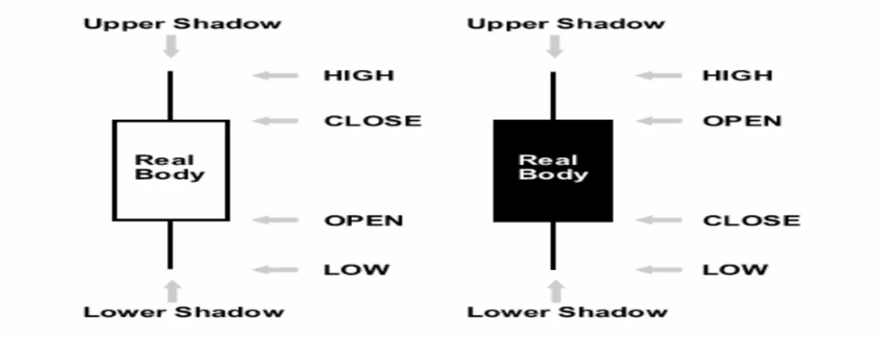
Answers (2006) further explain that when the body of the candlestick is white it signals that the closing price is higher than the opening price meaning that the price is going up. If the body of the candlestick is black it signals that the closing price is lower than the opening price meaning that the price is going down. The different variations are illustrated in the figure below. The length of the candlesticks is also important. The longer the candlesticks are “the more significant is the price change”.

Trading (2006) explain that the thin lines above and below the candlestick body are called shadows, wicks or tails. The names are the same for both the upper and lower part of the candlestick. The upper shadow is the high price and the lower shadow is the low for the period. Trading (2006) further explain that when we have candlesticks with small bodies and with long upper and lower shadows we have something called spinning tops. This means that the market is indecisive. The difference between the open and closing price was small: the market was in the end moving sideways. However the intraday price movement volatility from low to high was extreme. “Neither buyers or sellers could gain the upper hand”. A spinning top could be interpreted as a change in an ongoing trend.

StockChart (2006) compare candlesticks to a classical football game. A candlestick with a white body and “a long lower shadow would indicates that the Bears controlled the ball for a large part of the game but lost control by the end when the bulls made an impressive comeback”. This comeback by the bulls lead to a higher closing price which resulted in a long lower shadow. A candlestick with a white body and a long upper shadow would than indicate that the Bulls had control for a large part but lost control in the end to the Bears. This comeback by the Bears lead to lower closing price which resulted in a long upper shadow

Gump (2006) describes two reversal patterns called Hammer and Hanging Man which can be seen in the figure below. Both of the reversal patterns have at the top/bottom of the time series candlesticks with small black or white real bodies with long lower shadows. In the case of the Hammer we can see a small white candlestick with a long lower tail. As explained above this means that there was a strong selling pressure but in the end prices turned around and closed above the opening price. Gump (2006) further explain that the name hammer comes from “hammering out a new bottom”.

Figure 4 Reversal patterns (Gump, 2006)

Before we can act on the reversal we need some sort of confirmation. If a long white candlestick follows the hammer then we can interpret it as a confirmation that there is indeed a strong buying pressure, which would indicate a bullish reversal. The Hanging Man works in the same way with an initial strong selling pressure but in this case the prices do not turn around instead it closes below the opening price which is interpreted as a bearish signal. Also here we need confirmation that a bearish reversal is taken place in form of a long black candlestick. A hammer and Hanging Man with an upper long trail instead of a lower long trail could also be interpreted as a reversal pattern. The patterns are then called an inverted hammer vs. shooting star which is also illustrated in the above figure.

2.2 Stock Price Formations: B & R, Double- Triple Top and H & S

There are many different theories regarding price reversals for example: Bump and run reversal, double top reversal, triple top reversal and head and shoulder formations. In the text below some bullish price formation patterns will be described. The reader should notice that all these price formations also work in a bearish market. These bearish or bottom reversals will not be illustrated in order to decrease the volume of the theses. The bottom reversals works more or less in the same way but naturally in the opposite direction.

The historical price formations described here works as a basis for analysing and

understanding the current and future market. The most difficult thing is to correctly identify which of the different formations that will develop in the market. There is no easy way of knowing however if you know how the different formation looks like you could in the finishing phase of the formation correctly identify it and then profit from it.

The first price formation that will be presented is bump and Run (B & R) reversal. The bump and run formation is a result of that price is driven up too fast. The result is that there is no real support for the high price which leads to a fast decline. These types of markets are characterized by instability and speculation and can be rather destructive. Extreme bump and run reversals have historically been seen on average every fifth years.

Figure 5 Bump and Run Reversal (StockCharts, 2006)

Another formation called the double top reversal which is illustrated in the figure below. The double top reversal works more or less the same as the Bump and run formation. However here we clearly can see that the down trend is interrupted with a second up trend. Stockcharts (2006) explain that “the most important aspect of a double top reversal is to avoid jumping the gun”. An investor should wait until the support line is broken which is usually related to an expansion of volumes. Stockcharts (2006) further explain that “when the security does advance, look for a contraction in volume as an indicator of weakening demand”. As we say earlier stock price reversals are usually found after a strong uptrend in the market.

Figure 6 Double Top Reversal (Trade10, 2006)

A variation of the double top reversal is the triple top formation which is illustrated in the figure below. Daytrader (2006) explain that the formation starts with a simple uptrend that reaches point A. What we can see is that the “volume is increasing as the price move up.” After point A we will see the first v-formation A-B-C take place. The difference here is that the volume dose not increase at point B to C. This is the first warning signal that a down wards trend is developing. In second v-formation C-D-E we can see that the volumes continues to decrease in an upward trend and increases in downward trend. This is our second warning sign. At point E we can see that our triple top A-C-E has formed. Daytrader (2006) further explain that “once the price breaks the blue line the triple top is confirmed”. From point E and forward it is more or less downhill with increasing volumes as a result.

Achelis (2006) explain a fourth formation type the “Head-and-Shoulders (H & S) price pattern. The author explains that it is one of the most well-known chart patterns there is. It gets its name from the resemblance of a head with two shoulders on either side.” Stockcharts (2006) explain that the “pattern contains three successive peaks with the middle peak (head) being the highest and the two outside peaks (shoulders) being low and roughly equal”. The reason why the head and shoulder pattern are useful is because they resemble the way price trends typically reverse. The figure below illustrates how a head and shoulder reversal could look like in bull market.

Stockcharts (2006) explain that “the left shoulder forms a peak that marks the high point of the current trend. After making this peak, a decline ensues to complete the formation of the shoulder (1). The low of the decline usually remains above the trendline, keeping the uptrend intact.” Stockcharts (2006) further explain that “from the low of the left shoulder, an advance begins that exceeds the previous high and marks the top of the head. After peaking, the low of the subsequent decline marks the second point of the neckline (2)”.

Achelis (2006) describes that “the right shoulder is created as the bulls try to push prices higher, but are unable to do so. This signifies the end of the up-trend.” He also explains that a penetration of the neckline is interpreted as confirmation that a new down-trend will take place. After the penetration of the neckline it is common for prices to try to continuous the upward trend by trying to return to the neckline, as seen in the figure. However if the price is unable to return to the neckline it will usually result in a heavy price drop. A head and shoulder reversal in a bear market is illustrated in the figure below.

2.3 Eliot Wave Theory and Fibonacci Summation

Another theory about price formations is the Eliot wave’s formation. Stockcharts (2006) explain that Elliott wave theory basically says that “markets have well-defined waves that could be used to predict market direction. Stock prices also seams to be governed by cycles founded upon the Fibonacci series”. Fibtimer (2006) explain that Leonardo Fibonacci was a 13th century accountant that discovered the Fibonacci summation series. You start with the numbers 0 and 1, add them together and write down the sum. The series is continued by adding the previous two numbers. (If you take the ratio you will get the golden ratio, phi) The result is the following series: 0, 1, 1, 2, 3, 5, 8, 13, 21, 34, to infinity. According to Elliott wave theory all market moves can be described by five distinct upside waves and three distinct downside waves. The basic formations of the Elliot waves are illustrated in the figure below:

Figure 9 Eliot wave formation 1 (FutureInvestors, 2006)

Menttrading (2006) explain that “when traders are attempting to use the Elliot wave theory, one has to remember that it is a some what subjective type of analysis. If you are able to properly count the waves, they can provide great assistance”. However it is some times difficult with the untrained naked eye to exactly identify each of the waves. One example of a tool that could be used for pattern recognition and forecasting are neural networks that are becoming more and more advanced, interesting and effective. In the figure below the Elliot wave formation is illustrated for the NASDAQ Index.

2.4 Introduction to Moving Averages and MACD

Trade10 (2006) explain that moving averages are used as filters. MA reduces the white noise in the data which results in more clearly defined trends. A 20 day moving average represents the trend in prices over a period of 20 days. A long moving average is smoothed more than a short moving average. For a long moving average “each new day's data making less impact on the calculation of the moving average value compared to a shorter term moving average”. Trade10 (2006) explain that moving averages can be used as initial indicators of price trend. However an investment strategy that is only based on a moving average will most likely not produce any abnormal returns. Moving averages should therefore be used with other indicators or stop-losses to increase the reliability and security of the signals.

The periods of the moving average should be determined by the individual’s risk profile. Trader (2006) explain that “someone with a low risk profile and long-term strategies might choose slower moving averages, while someone willing to risk more might go for faster moving averages.” In the figure below a simple moving average with a two hundred day time-periods is illustrated.

Figure 11 Moving Averages (Zeal, 2006)

Chartfilter (2006) explain that investors could also use the moving average convergence/divergence (MACD) strategy. The MACD line is the difference between two exponential moving averages (EMA). One of the EMA is fast for example 12-day EMA and the other one is slower for example a 26-day EMA. The signal line is usually a 9-day EMA. Chartfilter (2006) explain that there are two MACD crossover signals: Signal line crossover that means that the MACD crosses above or below the signal line or the zero line (centerline) crossover that means that MACD crosses above or below the zero line. These two crossover signals are illustrated in the figure below. The basic MACD trading rule is to “buy when the

MACD rises above its signal line. Similarly, a sell signal occurs when the MACD crosses below its signal line.” If the zero line is also used a reference then an investor should according to Hirsch (2006) buy when the MACD graph is below the zero line (oversold) and the MACD line crosses the signal line from below and sell when the MACD graph is above the zero line (overbought) and the MACD crosses the signal line from above. Investopedia

(2006) explain a third trading signal “When the security price diverges from the MACD it indicate that the current trend is over”. A positive divergence is illustrated in the second figure below. StockCharts (2006) explain that “divergences are the least common of the three signals, but are usually the most reliable and can warn of an impending peak”.

Figure 12 Moving average convergence/divergence (ChartFilter, 2006)

2.5 Spurious Indicators: Traders Remorse and Bull Traps

MarketScreen (2006) explain something that they call Traders Remorse. Basically it is a falls indication that there is an upward trend in the market. Traders Remorse is the same thing as a “Bull Trap”. Stockcharts (2006) explain that a bull trap is “a situation that occurs when prices break above a significant level and generate a buy signal, but suddenly reverse course and negate the buy signal, thus "trapping" the bulls that acted on the signal with losses”. Traders Remorse occurs frequently when an investor uses moving averages as an investment strategy and especially when short time periods are used. The price crosses the moving average from below but directly after penetration it returns back to below the moving average. This is not good because it leaves a trader with a loss.

There are many different remedies to minimize the risk of Traders Remorse. An investor could for example use two or three moving averages with a small difference in time periods for example on nine period moving averages, one ten period moving average and one eight period moving average. The long/short period moving average works as a confirmation that there indeed is a strong upward/downward trend in the market. Another way of doing it, which is more or less the same as the previous one, is to assign the moving average with Bollinger bands that creates channels for the moving average for example a two standard deviations distance below and above either the price or the moving average. The Bollinger band works as a filter for interpreting the moving average crossovers.

Another way is to specify a percentage cross over strategy. An investor will not buy the security until it is for example 4% above or below its moving average. A fourth way that could be used includes the use of trend and momentum indicators such as Relative Strength Index (RSI), Relative Momentum Index (RMI) or Average Directional Index (ADX). These indicators will however not further be described in this thesis1_{. There is however some} additional problems related to all above described techniques. The above filters further increase the lag of our moving average indicator. The moving average will always be two steps behind but with an additional filter the investment strategy will be three steps behind which will increase the stability but reduce our potential profit.

Figure 14 Traders Remorse (MarketScreen, 2006)

2.6 Different Moving Averages and their Calculations.

There are many different types of moving averages. In this section a few of them will be described both from a technical and a more practical view. Trade10 (2006) explain that “the term "Moving" refers to the method of calculation which takes the average value over a fixed period of time and adds the latest period data to the calculation of the average while dropping the first period of the calculation so that the average continues to be calculated by the same number of periods but moves with each new period of data that occurs”. The starting point is a simple arithmetic moving average, which is illustrated below. (Cass, 2006)

1.1

Another useful moving average is called a weighted moving average which I illustrated below. Weighted moving average are useful because we can decrease the “lag” of a simple moving average by allocating more weights to the more recent prices than the ones that are longer back in time. Note that when the weights are equally distributed and sum to one, we will end up with a simple arithmetic moving average. (Cass, 2006)

1.2

Another variant is the simple geometric moving average which is illustrated below. The geometric average is more stable meaning that it is not as sensitive to volatility as the arithmetic simple moving average. Note that volatility usually is also a function of the time resolution. A dataset with a low time resolution usually have higher volatility than one with a high resolution, which is somewhat natural. We can also see that the log form of the simple geometric moving average is a simple arithmetic mean of the logged prices. (Cass, 2006)

1.3

Another variant is the exponential moving average that can be seen below. Willow (2006) explain that “exponential moving averages reduce the lag by applying more weight to recent prices relative to older prices which makes the exponential moving average more sensitive to a change in trend”. The smoothing constant (a) in the exponential moving average calculations below is a function of each of the observation in the defined range. There also exist many different variations of the Exponential moving average with somewhat different calculations. Sometimes the smoothing constant is calculated as 2/ (n+1) (Cass, 2006)

1.4 t t 1 t n 1 t P P P M n t n − − + + + + = ………… ≤ n i t i 1 1 t 2 t 1 n t n 1 i 1 t _n 1 2 n i i 1 w P w P w P w P W w w w w − + − − + = = + + + = = + + +

∑

∑

∏

3- Data and Method

The historical data from 1986-2006 on the S&P 500 index was extracted from the webpage of Yahoo finance. The data consisted of daily and monthly closing prices, volumes and dates. Motley (2005) explains that Standard & Poor 500 index is a market capitalization weighted index. This means that each companys market value is proportional to the index weight. This leads to that larger companies account for a greater share of the index. This is different from a price weighted index such as the Dow Jones Industrial Average that gives higher priced stocks more weight than lower priced stocks. “The S&P 500 represents approximately 70% of the value of the U.S. equity market. The 500 listed companies represent a diverse range of industries, spanning every relevant portion of the U.S. economy.

The larger amount of companies is one of the benefits of S&P-500 over Dow Jones Industrial Average. The index is comprised primarily of U.S.-based companies”. The S&P 500 index is an important indicator of overall US market performance. This is especially true for large cap stocks. The index work as an important benchmark of active portfolio fund managers to evaluate their performance compared to the overall stock market. “The companies that makes up the index represent 500 of the most widely held U.S.-based common stocks, chosen by the S&P Index Committee for market size, liquidity, and sector representation, leading companies in leading industries" is the guiding principal for S&P 500 inclusion”. “A small number of international companies that are widely traded in the U.S. are included, but the Index Committee has announced that only U.S.-based companies will be added in the future” (Motley, 2005).

Motley (2005) also explains that the S&P 500 have “significant liquidity requirements for its components, so some large, thinly traded companies are ineligible for inclusion. Because the index gives more weight to larger companies, it tends to reflect the price movement of a fairly small number of stocks”. This is also one of the index drawbacks. (Motley, 2005) Investors that want to follow the index dose not have to buy all 500 companies which would be quite hard. Instead they can buy exchange traded funds (ETF) called Spiders which tracks the S&P 500 index. In this thesis two different portfolios were constructed. The first portfolio Hugin was based on intraday data with a high time resolution. The second portfolio Munin was based on intramonth data with a lower time resolution. Further, the portfolios were constrained by two different types of stop losses one absolute and one trailing. The stop losses were only optimized on the first ten years from 1986 to 2006 in order not to over optimize the portfolio. The aim of this was to more realistically simulate the real world market environment by increase the uncertainty. The exact level of the stop losses was determined by iteration. A typical iteration process consisted with about 600 different trial and error simulations. The following optimization function was iterated, where T is the trailing stop-loss, A is the absolute stop- loss and P. R is the portfolio returns.

Max F~ (P. R) with respect to the constraints 0<T<50 & 0<A<50

The simulation assumed that the investor had an initial capital of 1,000 and was exposed to a 0.6 percent price slippage and transaction costs. The benchmark for the portfolios was the compounded average returns of the market over the last 20 year time period. The average market return was estimated at eight percent per year, which compounded over a 20 year period becomes 1000 * exp(0.08* 20) which is equal to approximately 2,225. If the portfolio returns minus the benchmark resulted in a positive number, we concluded that the selected portfolio and investment strategy indeed resulted in abnormal returns.

4- Empirical analysis

In the below sections as previously explained we assume that the investor have an initial capital of 1 K and is exposed to a 0.6 percent price slippage and transaction cost. We also assume that the investor takes both long and short positions in the market. Further he can only exit by the set stop-losses and he can only have one open position at a time. Our portfolio returns have to be higher than our benchmark of 1000*e^ (0.08*10) = 2 225

4.1 Optimization of the Hugin Portfolio, 1986-1996

We start with a simple 30 period MA cross strategy with no stop losses. The result of the trading strategy is presented in the table below.

Table 1 Hugin-portfolio with no stop-losses

All trades Long trades Short trades

Initial capital 1000.00 1000.00 1000.00

Ending capital 1003.89 997.59 1222.32

Net Profit 3.89 -2.41 222.32

Net Profit % 0.39 % -0.24 % 22.23 %

Exposure % 6.73 % 3.36 % 3.36 %

Net Risk Adjusted Return % 5.78 % -7.16 % 660.87 %

Annual Return % 0.04 % -0.02 % 2.05 %

Risk Adjusted Return % 0.58 % -0.73 % 61.04 %

Now we adjust the portfolio for optimal performance. We are using two types of stops here, one absolute stop-loss and one trailing profit stop loss. The code which is presented in the appendix-1 was written and implemented in order to optimize the investment strategy with the stop loses constraints. The default max, min and range of the stop loss constraint where estimated through trial and error in order to just visualize the critical areas of the charts. The result of the optimization process is illustrated in the figures below.

The charts illustrate the portfolio returns for different levels of the two stop-losses. The figure also identifies were the stable and unstable equilibriums are. You don’t want to over optimize, setting the stop-loss at an unstable point with enormous returns. A stable equilibrium with stable ROR is preferred from a stable investment perspective. The above 3D chart is compressed into a 2D graph in order to get a more clear visualization.

Figure 16 Optimized Stops for Hugin-Portfolio-2D

We can see that we can maximize the return with a trailing stop loss of 11 or with an absolute stop-loss of 1 however the points are non-stable. We therefore set the trailing profit stop loss= 24 and absolute stop-loss= 20. When we put in this in our model we get the following result presented in the table below. We can see that we have improved our trading result. Our net profit has increased. However, we are still not profitable. A further discussion of the different test statistics can be found in appendix-2.

Table 2 Hugin-portfolio after Optimization

All trades Long trades Short trades

Initial capital 1000.00 1000.00 1000.00

Ending capital 1908.40 1406.69 1717.74

Net Profit 908.40 406.69 717.74

Net Profit % 90.84 % 40.67 % 71.77 %

Exposure % 8.57 % 4.33 % 4.25 %

Net Risk Adjusted Return % 1059.94 % 940.27 % 1690.74 %

Annual Return % 6.76 % 3.52 % 5.63 %

4.2 Optimization of the Munin Portfolio, 1986-1996

We start with a simple 30 period MA cross strategy with no stop losses. The result of the trading strategy is presented in the table below.

Table 3 Munin-portfolio with no stop-losses

All trades Long trades Short trades

Initial capital 1000.00 1000.00 1000.00

Ending capital 1259.29 1215.73 1175.35

Net Profit 259.29 215.73 175.35

Net Profit % 25.93 % 21.57 % 17.54 %

Exposure % 2.52 % 1.68 % 0.84 %

Net Risk Adjusted Return % 1028.51 % 1283.61 % 2086.70 %

Annual Return % 2.37 % 2.01 % 1.66 %

Risk Adjusted Return % 94.05 % 119.32 % 197.04 %

Once again we adjust the portfolio for optimal performance. We are using two types of stops, one absolute stop-loss and one trailing profit stop loss. We run the same code but now on the monthly data in order to optimize the investment strategy with the stop loses constraints. The Figure below is a result of approximately 400 iterations.

Figure 17 Optimized Stops for Munin-Portfolio-3D

From the figure we can see that the highest returns are obtained by setting the trailing profit stop loss > 20. We can also see that the absolute stop-loss does not seam to matter for our portfolio returns. If we compare this chart with the previous one in the case of Hugin we can see that this one is more stable. In this chart we can see a large platform compared to many unstable peaks. We can see in the above figure that there is a clear structural break around a trailing profit loss of 20. To get a more clear visualization we check the 2D graph which is illustrated in the figure below. The chart confirmers our initial believes. The profits stops are therefore set at: absolute stop loss= 10 and trailing stop-loss at 23.

Figure 18 Optimized Stops for Munin-Portfolio-2D

When we put in the optimized stop levels in our model we get the following result presented in the table below. We can see also here that we have improved our trading result however we are still not profitable.

Table 4 Munin-Portfolio after Optimization

All trades Long trades Short trades

Initial capital 1000.00 1000.00 1000.00

Ending capital 1623.49 1623.49 1075.52

Net Profit 623.49 623.49 75.52

Net Profit % 62.35 % 62.35 % 7.55 %

Exposure % 56.34 % 56.34 % 0.00 %

Net Risk Adjusted Return % 110.67 % 110.67 % N/A

Annual Return % 8.65 % 8.65 % 1.25 %

4.3 Backtesting of the Hugin Portfolio, 1986-2006

Here our benchmark is 1000*e^ (0.08*20) = 4 953. By using the optimized stop-losses on the daily data (trailing= 24 and absolute= 20) on the whole trading period from 1986-2006 we get the following result presented in the figures below.

Table 5 Trading Result Hugin 1986-2006

All trades Long trades Short trades

Initial capital 1000.00 1000.00 1000.00 Ending capital 5098.15 5065.53 1514.95 Benchmark 4953.00 ** ** Overal Result +145.15 ** ** Net Profit 4098.15 4065.53 514.95 Net Profit % 409.82 % 406.55 % 51.49 % Exposure % 92.64 % 89.83 % 2.81 %

Net Risk Adjusted Return % 442.36 % 452.58 % 1831.53 %

Annual Return % 8.54 % 8.51 % 2.11 %

Risk Adjusted Return % 9.22 % 9.47 % 75.11 %

We can that the strategy indeed resulted in higher returns however the return was only marginal higher, +145.15. We can also check the trading statistics presented below.

Table 6 Trading Statistics Hugin 1986-2006

Max. trade drawdown -1544.90 -1544.90 -202.13

Max. trade % drawdown -25.01 % -25.01 % -18.86 %

Max. system drawdown -3622.25 -3623.76 -202.13

Max. system % drawdown -53.31 % -53.56 % -18.86 %

Recovery Factor 1.13 1.12 2.55

CAR/MaxDD 0.16 0.16 0.11

RAR/MaxDD 0.17 0.18 3.98

Profit Factor 3.47 3.45 N/A

Payoff Ratio 2.31 3.45 N/A

Standard Error 858.06 858.58 15.05

Risk-Reward Ratio 0.30 0.30 1.71

Ulcer Index 17.58 17.59 1.75

Ulcer Performance Index 0.18 0.18 -1.88

Sharpe Ratio of trades 0.21 0.22 N/A

4.4 Backtesting of the Munin Portfolio, 1986-2006

Also here our benchmark is 1000*e^ (0.08*20) = 4 953. By using the optimized stop-losses on the monthly data (trailing= 23 and absolute= 10) on the whole trading period from 1986-2006 we get the following result presented in the figure below.

Table 7 Trading Result Munin 1986-2006

All trades Long trades Short trades

Initial capital 1000.00 1000.00 1000.00 Ending capital 4607.82 4607.82 1231.49 Benchmark 4953.00 ** ** Overal Result -345.18 ** ** Net Profit 3607.82 3607.82 231.49 Net Profit % 360.78 % 360.78 % 23.15 % Exposure % 74.38 % 74.38 % 0.00 %

Net Risk Adjusted Return % 485.02 % 485.02 % N/A

Annual Return % 9.49 % 9.49 % 1.24 %

Risk Adjusted Return % 12.76 % 12.76 % N/A

We can that the strategy did not result in any abnormal returns, -348.18. We can also as previously check the trading statistics which are presented below.

Table 8 Trading Statistics Munin 1986-2006

Max. trade drawdown -1390.95 -1390.95 0.00

Max. trade % drawdown -23.55 % -23.55 % 0.00 %

Max. system drawdown -1390.95 -1390.95 0.00

Max. system % drawdown -23.55 % -23.55 % 0.00 %

Recovery Factor 2.59 2.59 N/A

CAR/MaxDD 0.40 0.40 N/A

RAR/MaxDD 0.54 0.54 N/A

Profit Factor N/A N/A N/A

Payoff Ratio N/A N/A N/A

Standard Error 606.21 606.21 2.23

Risk-Reward Ratio 0.49 0.49 6.19

Ulcer Index 8.42 8.42 0.00

Ulcer Performance Index 0.49 0.49 N/A

Sharpe Ratio of trades N/A N/A 0.00

5-Conclusions

Previous studies have drawn different conclusions whether technical analysis results in an extra edge in the market. My conclusion regarding the use of technical analysis and especially the 30 period moving averages is presented below. The reader should note that neither Hugin nor Munin did produce abnormal returns without the optimized stop losses. Further after backtesting the different portfolios it is clear that the more trades that are involved the more sensitive the results is to the assumption of the transaction cost. This is especially true when it comes to the Hugin portfolio. Altering the level of transaction costs will also most likely affect the outcome of the trading result

Will a 30 period MA with optimized stop-losses produce abnormal return for Hugin?

By optimizing the trading stops an investor would have increase the net profit compared to the non optimized portfolio. Further an investor taking a long position in S&P-500 for twenty years and reinvesting all profits in the portfolio would have received on average a compounded net profit of _1,000*e0.08*20_{-1,000 3,953}= If an investor would have used a 30 period MA with optimized stop-losses he would have produced a net profit of 4,098 approximately a four percent improvement. We can see that the strategy was profitable however the interpretation is not as straightforward as it first appears. The daily portfolio would by assumption require a higher return since a much more active role would be assumed by the investor. An investor has to daily monitor the portfolio mechanics for twenty years which naturally would be related to large costs.

Will a 30 period MA with optimized stop-losses produce abnormal return for Munin?

If an investor would have used a 30 period MA with optimized stop-losses he would not improved his trading result for the monthly portfolio compared to a long position. Does this mean that a 30 period MA could never successfully be applied on monthly basis? No it does not. The monthly portfolio has naturally a higher volatility and we also know that the period between 1996-2006 have had a higher volatility than the years 1986-1996. This result in that a monthly portfolio where the stop losses were optimized on the entire time period or a portfolio with stricter set stop losses would maybe have produce better results. However from a stable investment strategy perspective an investment strategy should work regardless of the time frame or individual market specifics.

Further Studies

Other theses could analyze other investment strategies based on technical analysis or any other investment strategy. Other more complex investment strategies with a combination of different indicators could also be investigated. Numerous anomalies in the market could also be tested and evaluated. Some examples IPO-effects, reversion of the mean, neglected firm effect, post earning announcement drift effect, value vs. growth or small firm effect

References

Achelis, S (2006) Technical Analysis from A to z, extracted 2006-03-01 from http://www.equis.com/free/taaz/inttrends.html

Amibroker (2006) Technical Analysis extracted 2006-03-08 from http://www.amibroker.com/ Answers (2006) Candelsticks extracted 2006-04-04 from

http://www.answers.com/topic/candlestick-chart

Cass (2006) Commodity Risk Management extracted 2006-04-01 from

www.cass.city.ac.uk/faculty/m.tamvakis/files/CRM_Lec2_Technical_analysis.ppt Chartfilter (2006 MACD extracted 2006-02-06 from

http://www.chartfilter.com/reports/c22.htm

Cheol-Ho & Irwin (2004) The Profitability of Technical Analysis: A Review, AgMAS Project Research Report

Daytrade (2006) Tripel Top Reversal extracted 2006-03-28 from

http://www.daytradeteam.com/dtt/swing-trading-strategy/2005/10/triple-top-reversal-patterns-technical.html

Fama, E (1970) “Efficient Capital Markets: A Review of Theory and Empirical Work.”

Journal of Finance, 25:383-417.

Fibtimer (2006) Basics of Fibonacci ratios and Elliott wave theory extracted 2006-03-01 from http://www.fibtimer.com/subscribers_historical_reports/050130_fibtimer_commentary.asp FutureInvestors (2006) Elliott Wave Introduction extracted 2006-03-01 from

http://www.futures-investor.co.uk/elliott_wave_intro_1.htm

Gump (2006) Trading Japanese Candlesticks extracted 2006-04-05 from http://www.babypips.com/forex-school/japanese-candlesticks.html

Hirsch (2006) Applying the MACD indicator to our best six month strategy extracted 2006-02-26 from http://www.hirschorg.com/default.asp?action=macd Investopedia (2006) MACD extracted 2006-02-26 from

http://www.investopedia.com/terms/m/macd.asp

Levich, R &Thomas, L (1993) “The Significance of Technical Trading-Rule Profits in the Foreign Exchange Market: A Bootstrap Approach,” Journal of International Money and Finance, October, pp. 451-74.

MarketScreen (2006) Support and Resistance extracted from 2006-04-10 from http://www.marketscreen.com/help/AtoZ/default.asp?hideHF=&Num=9 Menttrading (2006) Elliot Wave Basics extrated 2006-03-01 from http://www.ment.com/training/TA_EW3.htm

Motley, (2005) Motley Fool Index Centre, extracted 2005-10-06 from http://www.fool.com/school/indices/sp500.htm

Samuelson, P (1965). “Proof That Properly Anticipated Prices Fluctuate Randomly.”

Industrial Management Review, 6:41-49.

Satchwell, C (2005) Pattern Recognition and Trading Decisions, McGraw-Hill StockCharts (2006) Head and Shoulder extracted 2006-02-26 from

http://www.stockcharts.com/education/ChartAnalysis/headShouldersBottom.html Trader (2006) Moving averages extracted 2006-03-26 from http://www.option-trading-guide.com/movingaverages.html

Traders-edge (2006) The trend is your friend extracted 2006-05-30 from http://www.tradersedgeindia.com/trend_is_your_friend.htm

Trade10 (2006)Moving Averages extracted 2006-02-26 from http://www.trade10.com/Moving_Average.html

Willow (2006) Calculating Exponential Moving Averages extracted 2006-04-10 from http://www.willowsolutions.com/tips/tips_2002_11_1.shtml

Appendix

Appendix 1

Optimization and Backtesting code

AddTextColumn(FullName(),"Name");

AddColumn( C, "Close" );

AddColumn( C - Ref( C, -1 ), "Change" );

AddColumn( V, "Volume", 1 );

AddColumn( High, "High");

AddColumn( O, "Todays Open");

ApplyStop(stopTypeTrailing, stopModeRisk, Optimize( "Trailing-Profit-Stop", 0, 1, 40, 2 ), True );

ApplyStop(stopTypeLoss,stopModePercent, Optimize( "Stop-loss", 0, 1, 30, 2 ), True );

Buy = Cross (Close, MA( Close, 30 ) );

Sell = Cross (MA( Close, 30 ), Close );

Filter=Buy OR Sell; SetTradeDelays(0,0,0,0);

Cover=Buy; Short=Sell;

Appendix-2

Explanation of Statistics (Amibroker, 2006)

Exposure % - 'Market exposure of the trading system calculated on bar by bar

basis. Sum of bar exposures divided by number of bars. Single bar exposure is the

value of open positions divided by portfolio equity.

Net Risk Adjusted Return % - Net profit % divided by Exposure %

Annual Return % - Compounded Annual Return % (CAR)

Risk Adjusted Return % - Annual return % divided by Exposure %

Avg. Profit/Loss - (Profit of winners + Loss of losers)/(number of trades)

Avg. Profit/Loss % - (% Profit of winners + % Loss of losers)/ (number of

trades)

Avg. Bars Held - sum of bars in trades / number of trades

Max. Trade drawdown - The largest peak to valley decline experienced in any

single trade. The lower the better

Max. Trade % drawdown - The largest peak to valley percentage decline

experienced in any single trade. The lower the better

Max. System drawdown - The largest peak to valley decline experienced in

portfolio equity. The lower the better

Max. System % drawdown - The largest peak to valley percentage decline

experienced in portfolio equity. The lower the better

Recovery Factor - Net profit divided by Max. system drawdown

CAR/MaxDD - Compound Annual % Return divided by Max. system %

drawdown. Good if bigger than 2

RAR/MaxDD - Risk Adj Return divided by Max. system % drawdown. Good if

bigger than 2

Profit Factor - Profit of winners divided by loss of losers

Payoff Ratio - Ratio average win / average loss

Standard Error - Standard error measures chopiness of equity line. The lower the

better.

Risk-Reward Ratio - Measure of the relation between the risk inherent in a

trading the system compared to its potential gain. Higher is better. Calculated as

slope of equity line (expected annual return) divided by its standard error.

Ulcer Index - Square root of sum of squared drawdowns divided by number of

bars

Ulcer Performance Index - (Annual profit - Tresury notes profit)/Ulcer

Index'>Ulcer Performance Index. Currently tresury notes profit is hardcoded at

5.4. In future version there will be user-setting for this.

Sharpe Ratio of trades - Measure of risk adjusted return of investment. Above 1.0

is good, more than 2.0 is very good. More information

www.stanford.edu/~wfsharpe/art/sr/sr.htm Calculation: first average percentage

return and standard deviation of returns is calculated. Then these two figures are

annualized by multipling them by ratio (NumberOfBarsPerYear)/

(AvgNumberOfBarsPerTrade). Then the risk free rate of return is subtracted

(currently hard-coded 5) from annualized average return and then divided by

annualized standard deviation of returns.

K-Ratio - Detects inconsistency in returns. Should be 1.0 or more. The higher K

ratio is the more consistent return you may expect from the system. Linear

regression slope of equity line multiplied by square root of sum of squared

deviations of bar number divided by standard error of equity line multiplied by

square root of number of bars. More information: Stocks & Commodities V14:3

(115-118): Measuring System Performance by Lars N. Kestner