China's regional inflation
An empirical study of Phillips curveMaster thesis within Economics
Author: Yilin Jiang
Tutor: Börje Johansson
Ass. Tutor: Erik Wallentin
Master Thesis in Economics
Title: China’s Regional inflation – An empirical study of Phillips Curve
Author: Yilin Jiang
Supervisors: Börje Johansson; Erik Wallentin
Date: 2015
Keywords: Inflation, unemployment, GDP, Phillips curve, divergent
Abstract
This thesis is aimed at investigating the situation of divergent inflation rates of all provinces in China by the year 2000 to 2013. In order to investigate whether inflation is divergent in China, the study establishes a modified Phillips Curve model, to verify whether the Phillips curve is applicable to China, whether the provinces’ inflation rates are displaying a similar sensitivity to changes in unemployment or the output gap as the average of China. This study uses the Panel Least Square for all provinces, and the time series is used to test for each province compared with average of China separately. The result shows that the provincial inflation rates have different sensitivity to changes in the output gap compared with the average of China. Additionally, the original Phillips curves and modified Phillips curves are applicable for provinces of China when the fixed effect at regional level.
Table of Contents
Abstract...2
1 Introduction ...4
2 Theoretical Framework and Background...7
2.1 Previous research on regional disparity in China...7
2.2 Inflation studies ...8
2.3Original Phillips Curve ...9
2.3 Evolution of the Phillips Curve ...12
3 Empirical Study ...13 3.1 Econometric Model...13 4.2 Data selection ...15 4.3 Empirical investigation...16 5 Empirical Results...17 6 Conclusions ...24 References ...26 Internet database...27 Appendix A...27 Appendix B ...28 Appendix C ...28
1 Introduction
Since the end of last century, economic reforms brought China a powerful vitality. In order to promote economic development, the Chinese government adjusted its economic strategy shift from a planned economy to a market economy, gradually establish an open market environment. In this context, China has a rapid economic progress, especially in the beginning of this century. According to Figure 1.1, we can clearly recognize the China's GDP growth rate for the past ten years.
Figure1.1: GDP Growth of China (from 2005-2014)
Rapid economic growth has also brought some problems, such as fluctuations of inflation and unemployment,
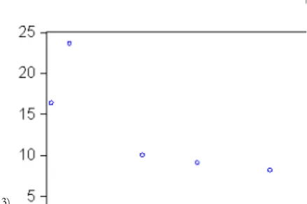
According to the data given by China Statistics Bureau, since the beginning of this century, the national unemployment rate rose by 1 percent. However, the inflation rate has stabilized. Figure 1.2 illustrates Retail Price Index (RPI) of China from 1993-2013. The retail price index takes into account the change in retail price of goods and the extent of the trend in a period of time. Retail Price Index is related to the national revenue, balance of market, consumption and accumulation. This index is used to identify the rate of inflation. At first glance, the volatility of the Index of Retail Price Index (RPI) was extremely high, but it's becoming stabilized since the end of last century, fluctuating between the intervals of -1% to 5%.
1993 1994 1995 1996 1997 1998 1999 2000 2001 2002 2003 2004 2005 2006 2007 2008 2009 2010 2011 2012 2013 -5 0 5 10 15 20 25
Retail Price Index
Figure1.2: Index of Retail Price of China (from 1993-2013)
In addition to the economic progress in national level, the difference between Chinese provinces is also becoming increasingly clear.
China is in possession of 34 provincial-level administrative regions. There make two components of the governance system in China: political centralization and economic regional decentralization (Xu 2011). The political centralization system means higher level officials control over their lower level counterparts in the hierarchical administrative system. The higher level officials to evaluate the lower level officials based on their performance (Yu, Zhou& Zhu 2014). The higher level officials are willing to promote the lower level official based on his good performance for the local economy. For example, a good performance, such as increasing GDP growth that can improve low level official’s evaluation. In this case, all lower level officials joining a ‘tournament competition’ of promotion, because opportunity for promotion depends on their performance. On the other hand, local officials have a great deal of power for enhancing the local economy, which is so-called regional economic decentralization.
Let us compare the tournament competition among native officials in China with Western style yardstick competition (Besley& Case 1995) The assessment of yardstick competition is decided on voters, it's a bottom-up power structure of a democratic approach. In China, the tournament competition depends on the choice of high-level officials, it's a top-down power structure.
Based on economic decentralization (Yu, Zhou& Zhu 2014), local officials are able to leverage investment in the governmental instruments. For example, local officials could influence the investment decisions of state-owned enterprises by administrative order. They allocate loans from local state-owned banks, and give low-interest loans to establish a pro-business policy and services. Local officials also give a low tax rate for foreign enterprises and factories. Local officials aim to attract FDI and investment from other regions (Yu, Zhou& Zhu 2014).
Yu, Zhou& Zhu (2014) researched Prefectural-city level total investment. They find that the spatial correlation between cities in the same province is concentrated. Correlation between cities that are geographically proximate but situated in different provinces are weak. The promotion of local city leaders is voted on the provincial government. In other words, each province has independent decide for economic growth.
In this case, because of differences in respective administrative measures and the region's environment, differences in economic development among various regions are inevitable
Different from nationwide economic growth, the regional economic disparities between regions performed in different fields. Scholars have already examined regional economic disparities, such as investment disparity (Chun-Hung 2011), income inequality (Ding 2008), trade disparity (Zhenhui 2012) and inflation disparity (Aviral& Suresh 2012). The most previous research has been brought on the case of European countries, examining the impact on a unified currency for each country. For example, Nilsson (2011) researched divergent inflation in Euroland by means of the Phillips Curve. My thesis opens a new perspective, built on the background of regional economic and political governance system. It considers each province of China as an independent economy, to clarify the relationship between the provincial economy and the national economy.
The hypothesis of this research: whether the Phillips curve applies to China; if the provincial inflation rate movement is significantly different from the average of China, the large economy China is facing an invisible inflation divergence. Therefore, each province is more independent from the beginning of this century.
Building on existing research, my study aims at pushing the research of regional economic disparity further by changing the inflation rates. I will use the Phillips curve to test the difference between national inflation and provincial inflation. Through creating a model, I will investigate how changes in unemployment affect inflation at both provincial and national levels. Then come if the Phillips curve applies to the case of China in accordance with the final result
The purpose of this paper is investigating if changes in unemployment or output gap for provinces affect the inflation rate for a similar way of the average of China. Furthermore, it aims to test if the provincial inflation rate is convergent with national inflation since the beginning of this century; and how is the sensitivity of inflation. Finally, whether the Phillips curve is suitable for the case of China.
The paper outlined as follows: the next section reviews some relevant literature of regional diversities of China. Furthermore, it briefly discusses the Phillips curve, the relationship between inflation and unemployment. With regard to the inflation rates of
China, the third section examines the provincial inflation trend. Section four inspects the empirical analysis and then works out the results. At last the paper ends with a conclusion in the final section.
2 Theoretical Framework and Background
2.1 Previous research on regional disparity in China
China is one of the most important economies in the world. This section briefly introduces regional disparities in China through an economic lens.
Scholars noticed China's regional disparity in investment, especially for foreign direct investment since 1990. Foreign direct investment impact on regional economies are unequal in China. In order to study the effect of foreign direct investment of regional productivity in China, Chun-Hung (2011) adopted a measure of total factor productivity (TFP). According to Chun-Hung's research, he deal with the endogenous inputs choice accompanied by various measures of investment, thereby to provide robust estimates on the TFP effect of FDI. Building on the provincial level of panel dataset over the time period 1997–2006, the difference in productivity effect of FDI between coastal and non-coastal regions is also examined. The results show that the overall productivity effect of FDI is positive, and this effect is much depends on the absorptive ability of the host region. In addition, Chun-Hung found a technological gap which is linked with the finding. It means investment has a higher impact on productivity in coastal regions instead of their non-coastal, because coastal regions tend to have better technology (Chun-Hung 2011). To sum up, Chinese government should continue to attract foreign direct investment, and provide incentives to upgrade multinational Chinese subsidiaries of its production. From the perspective of promoting productivity, FDI should consider what type of technology is suitable, instead of focus on attracting technology intensive FDI. Secondly, innovation activities are a major factor of technological progress. In order to create local technological capabilities, both public and private sector committed to innovation activities more attention
Kang (2011) examined the regional stock of foreign direct investment to test regional income inequality. From 1990 to 2005, the stock of investment has contributed less to two percent of regional income inequality. At the same time, provincial per capita tangible assets account for over fifty percent of income inequality which contributes to sixty five percent of the increases in income inequality. Other significant determinants of regional income inequality are due to the location of the province and educational level (Kang 2011).
Zhang (1999) built a mathematical model with Gini coefficients which was utilized to study the time series properties of China's regional income differences. The Gini coefficient is a numerical aggregate measure of income inequality ranging from zero to one. The greater the value of Gini coefficient, the larger inequality of income distribution. The result shows that from 1952 to 1978 the differences become larger; from 1978 to the beginning of 1990s decreases; from the beginning of 1990s to 1995 the difference slightly increases. Regional income inequality is an inevitable phenomenon in China.
Regional trade is influenced by several factors, such as costs of transportation, income level (Xu, Fan 2012). Li and Hou (2008) investigated trade border effects in China’s regional markets, depending to the gravity model. Except income and distance, other factors, such as the effects of intra-industry trade, transportation costs, and investment environment of regional trade and border effects are also associated with regional trade. Since the global economic crisis in 2007, China moves from export-led growth to promote domestic demand. Xu and Fan (2012) used Anderson and Wincoop (2003)' methodology to examine China’s domestic market integrations. The border effects of national level and regional levels are significantly different (Xu & Fan 2012). Remarkably, income growth, lower transportation costs, and higher intra-industry trade is positive for regional trade.
In summary, each region of China reflects the disparity in economic development. These huge regional differences impact on inflation, unemployment and other economic indicatorsaround the country.
2.2 Inflation studies
In addition to income, foreign direct investment and trade flows, inflation is equally a focus of research scholars. Inflation is affected by many factors, and it’s represented by different indicators. He and Fan try to find measurable indices of China’s inflation, and by establishing a model to predict China's inflation rate (He & Fan2015)
He and Fan believes that to investigate inflation, people need consider several factors. First, the inflation rate contains only factor lagging autoregressive model. The essence of this model is using their past behavior to predict future behavior of inflation. The advantage of this method is simply; but the drawback is that it is not a strong sense of economic theory, hence, this model cannot fully reflect the impact of other economic variables on inflation. Phillips curve is a classic model of inflation.
The quantity theory of money serves as a model for researching the inflation rate. Some knowledge and experience have been devoted to the quantity theory of money, but its effectiveness has been disputed by some scholars. Some scholars find that money does not have long-run effects on inflation; and the inflation rate can be interpreted by
monetary growth since there is no strong relationship between the two factors. But others scholars, find that there is a significant relationship between inflation rate and the money supply. For example, McKinnon (2014) supposes the monetary control has a significant effect for inflation.
Phillips curve is a classic model of inflation. The current study of Phillips curve shows a positive output gap means that inflationary pressure is growing. I will explain the details of this theory in the next subsection.
Based on the basic theories, Ching and Chun investigate the possibility of predictivity of three dimension reduction techniques used in a data-rich environment. They used Principal Components Analysis (PCA), Sliced Inverse Regression (SIR), and Partial Least Squares (PLS) applied in the Factor-Augmented Auto-regression (FAAR) model. Collecting data from January 1998 to December 2009 in China to construct factors for use by three different techniques. The performance of different dimension reduction methods depends on forecasting horizons, the number of factors chosen, and the number of slices for SIR. The results show the FAAR model with 11 PCA factors is the optimal one to the other models about inflation forecasting in China. (Ching & Chun 2013).
2.3Original Phillips Curve
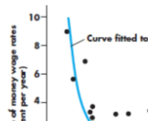
In 1958, William Phillips researched relationship between unemployment and money wage rate, according to the variations of unemployment and money wage rates during 1861-1913 in Britain. Based upon unemployment rate and the money wage change rate, Phillips (1958) made a graph to represent the relationship between unemployment and money wage rate. In figure 1, a curve shows if the unemployment rate is lower, growth rate of money wages is higher. On the contrary, when the unemployment rate is elevated, it's lower the growth rate of money wages, or even negative. According to the theory of cost-push inflation, the inflation rate can be written in money wages. Therefore, this curve can be expressed alternatively relationship between unemployment and inflation. Namely, high unemployment means that the economy is in a recession phase, where the level of wages and prices is low, so there is a low rate of inflation. Conversely low unemployment rate indicating that the economy is in the boom phase, both wage and price levels are high, thus inflation is also high. There is an opposite direction of the relationship between unemployment and inflation.
Figure 1: The original Phillips curve for the United Kingdom (Dornbusch, Startz, Fischer 2008)
Phillips curve implies a rate of change of money wage rates can be explained by the level of unemployment and the rate of change of unemployment.
𝑔𝑤=𝑊𝑡 + 1𝑊‒ 𝑊𝑡
𝑡 (1)
In equation 1, where 𝑊𝑡is the wage of this period; 𝑊𝑡 + 1is the wage of the next period
𝑔𝑤 denotes the rate of wage inflation, which is negatively related to the wage of period t, but positively related to the wage in the next period t+1.
Based on figure 2.3.1, to improve the equation 1, we need consider the natural rate of unemployment. Let 𝑢∗be the natural rate of unemployment; 𝑢 is the unemployment rate, ε is the coefficient which represents the effect of inflation movement. The new equation is:
𝑔𝑤=‒ ε(𝑢 ‒ 𝑢∗) (2)
Equation 2.2.2 states that wages are falling when the unemployment rate exceeds the natural rate (𝑢>𝑢∗). (𝑢 ‒ 𝑢∗) is the so-called 'unemployment gap'.
Next step, Phillips curve indicates that the relationship between unemployment and inflation rates, it is an ‘unemployment - price’ Phillips curve. Inflation rate substitute the rate of change of money wage rate. The substitute is achieved through an assumption. This assumption mean: price per unit of product is equal to the average labor cost plus other fixed costs and profits. This Phillips curve is similar to equation 2, except that wage
inflation was replaced by price inflation. Increasing inflation can promote employment. Based on the given relationship, a linear equation is expressed as:
π =‒ φ(𝑢 ‒ 𝑢∗) (3)
The equation 3 illustrates the relationship between inflation and unemployment. π represents inflation; φ is the coefficient which represents the effect of inflation movement;𝑢 is the unemployment rate; 𝑢∗ denotes the natural rate of unemployment. Equation 3 is a simple Phillips curve relationship, it means the basic relationship between inflation and unemployment.
In equation 3, the Phillips curve only contains the inflation rate without the expected inflation. Because it does not take into account people's expectations of inflation. Friedman (1968) raised expectations-augmented Phillips curve, he believes the original Phillips curve confused nominal wage rates and real wage rate, the real wage rate determines the labor supply and demand. Therefore, Friedman added price expectations. Firms and workers are concerned with the real value of the wage, so they would like to adjust the level of the nominal wage to forecast the expected inflation. In this case, the Phillips curve should reconsider the unemployment and add expected inflation. The equation 3 can be derived to:
(𝑔𝑤‒ π𝑒) =‒ φ1(𝑢 ‒ 𝑢∗) (4)
In equation 5, π𝑒denotes the expected price inflation in the previous period. In this case, when the inflation is change, unemployment and future expectations of inflation also changed. We suppose in time period t, the expected inflation equal to the inflation in time period t-1, π𝑒= π𝑡 ‒ 1. Actually, this equation cannot be completely accepted,
because expectations are not depending on only past experiences. According to the assumption of a constant real wage, actual inflation π will equal to wage inflation. The expectations-augmented Phillips curve is (Dornbusch, Startz, Fischer 2008):
Equation 2.2.5 will be utilized in the empirical study.
2.3 Evolution of the Phillips Curve
The relationship between economic growth and inflation rate can be termed to output - price Phillips curve. This Phillips curve uses economic growth instead of the unemployment rate of the previous Phillips curve.
Friedman's expectation and the natural rate of unemployment are expected to change the original Phillips curve. Money illusion is a factor which has not been taken into account. It means people just react to the nominal value of the currency, while ignoring the real purchasing power of currency is changing. Friedman removes inflation and unemployment in the original Phillips curve, and selects the employers and workers. It results from money illusion Short-term substitutes (Friedman 1967). For the long term, everyone will adjust to the correct expectations, changes from nominal demand will have no impact on the unemployment rate. Natural rate of unemployment affecting the development of relevant theories
Any negative correlation between inflation and unemployment, is called Phillips curve effects (Lucas 1969). The relationship between inflation and real output is called the deformation of the Phillips curve (Lucas 1972)
Lucas’s theory of the Phillips curve is to a great extent inherited from Friedman's natural rate of unemployment. In his framework, economies are pursuing the optimization principle to settle the problem, and therefore money illusion is disappeared. Therefore, he believes money should not lead to changes in the real variables change. On the contrary, there is a positive correlation between inflation and real output. Thus, the unemployment rate gap may be amended by replacing industrial gap, negative inflation rate and unemployment change to the positive correlation between inflation and the output gap. The original Phillips curve became aggregate supply curves, the relationship between the money market and the labor market became the relationship of the money market and commodity markets.
In 1962, Arthur Okun found a fixed relationship between the unemployment rate and the output gap.
𝑢 ‒ 𝑢∗ =‒ 𝑎(𝑦 ‒ 𝑦
∗
𝑢∗ denotes the natural rate of unemployment, 𝑦∗ denotes potential output/potential economic growth rate, 𝑦 denotes real output/real economic growth rate. This equation 6 is called Okun's law. Okun's law describes a fairly stable relationship between changes in GDP and unemployment change. This theory demonstrates that unemployment rate and GDP growth rate are negatively related. Depending on Okun's law, output gap/economic growth replaces the unemployment gap, and the Phillips curve can easily be converted to the aggregate supply curve. Equation 5 can be derived to:
π = φ3
(
𝑦 ‒ 𝑦∗
𝑦∗
)
+ π𝑒
(7) Based on equation 7, inflation is positively related to real output, but negatively related to potential output. Equation 7 will be used in this thesis as an alternative method of empirical study.
For China, the empirical research of the Phillips curve is more difficult. Because China's economic reform is still underway, so we cannot simply use one model to ensure whether it satisfied the conditions of the Phillips curve. Hence, I will use different Phillips curve models in the section of the empirical study.
3 Empirical Study
3.1 Econometric Model
The Phillips curve was utilized to test a negative relationship between unemployment and inflation rate. In this case, the empirical study analyzes whether changes in unemployment for regions affect the inflation rate similar to the average of China. Furthermore, ‘Phillips coefficient’ which represents the coefficient between unemployment and inflation will be investigating whether it differ in 30 provinces of China. How provincial unemployment changes to affect inflation rates across China. Panel data will be utilized in this section. The advantage of the panel data analysis which contains the cross sectional data and time series data. In this empirical study, the cross sectional term is the 30 provinces of China, time series is the time period from 2000 to 2013 (annual data).
To test whether the Phillips coefficient of the province is different from the average of China, I derive a model from the basic Phillips curve equation 3.First, we consider the Phillips curve which reflects the relationship between unemployment and inflation. And then, we assume both provincial Phillips curve and average of China’s Phillips curve
merged into one equation. Then we can compare these two Phillips curves through a parameter.
π𝑗,𝑡= π𝑗,𝑡𝑒 ‒ φ𝑗(𝑢𝑗,𝑡‒ 𝑢∗𝑗) (3.1.1)
Equation 3.1.1 represents the Phillips curve for a province. π is the inflation rate, π𝑒denotes expected price inflation in the previous period, 𝑢 is the unemployment rate, j denotes the province, t denotes time period, 𝑢∗ represents the natural rate of unemployment
π𝑎𝑣𝑒,𝑡= π𝑎𝑣𝑒,𝑡𝑒 ‒ φ𝑎𝑣𝑒(𝑢𝑎𝑣𝑒,𝑡‒ 𝑢𝑎𝑣𝑒∗ ) (3.1.2)
Equation 3.1.2 is the Phillips curve for average level of China. π𝑗,𝑡 π𝑎𝑣𝑒,𝑡= λ ‒ φ𝑗 φ𝑎𝑣𝑒( 𝑢𝑗,𝑡‒ 𝑢∗𝑗 𝑢𝑎𝑣𝑒,𝑡‒ 𝑢𝑎𝑣𝑒∗ ) + ( π𝑗,𝑡𝑒 π𝑎𝑣𝑒,𝑡𝑒 ) (3.1.3)
Equation (3.1.3) is merged from (3.1.1) and (3.1.2). λ is the intercept, φ is a negative
Phillips coefficient, ave denotes the average of China,. π𝑗,𝑡𝑒
π𝑎𝑣𝑒,𝑡𝑒 is the variable of future
expectation of inflation. φ𝑗
φ𝑎𝑣𝑒 is the coefficient to test whether two Phillips coefficients
are different. If Phillips coefficients is different, φ𝑗
φ𝑎𝑣𝑒 will be different from 1. This means the provincial inflation is not 100% sensitive to the average of China to the changes of unemployment.
Set a lagged one period as a control variable for the expectation of inflation π𝑗,𝑡𝑒
π𝑎𝑣𝑒,𝑡𝑒 . Then the equation (3.1.3) can be formulated as:
π𝑗,𝑡 π𝑎𝑣𝑒,𝑡= λ ‒ φ𝑗 φ𝑎𝑣𝑒( 𝑢𝑗,𝑡‒ 𝑢∗𝑗 𝑢𝑎𝑣𝑒,𝑡‒ 𝑢𝑎𝑣𝑒∗ ) + ω( π𝑗,𝑡 ‒ 1 π𝑎𝑣𝑒,𝑡 ‒ 1) (3.1.4)
ω is the coefficient on future expectation of inflation. Before running the regressions, the ratios of inflation (
π𝑗,𝑡
π𝑎𝑣𝑒,𝑡) and unemployment (
𝑢𝑗,𝑡‒ 𝑢∗𝑗
𝑢𝑎𝑣𝑒,𝑡‒ 𝑢𝑎𝑣𝑒∗ ) should be worked out. Equation (3.1.4) can be simplified as:
̃π𝑗,𝑡= λ ‒ φ
(
̃𝑢𝑗,𝑡)
+ ω(
̃π𝑗,𝑡 ‒ 1)
+ α𝑗+ ε𝑗,𝑡 (3.1.5)α𝑗 is the fixed effect of each province, ̃𝑢𝑗,𝑡 is equal to
𝑢𝑗,𝑡‒ 𝑢∗𝑗
𝑢𝑎𝑣𝑒,𝑡‒ 𝑢𝑎𝑣𝑒∗ . It denotes the ratio of unemployment between the specific province and average of China. For the natural rate of unemployment, it is unobservable, so the natural rate of unemployment cannot be shown separately, we assume it is incorporated into specific fixed effects α𝑗. In this case,
these are another promising estimation if the fixed effect of different time period is contained. Equation 3.1.5 transforms to:
̃π𝑗,𝑡= λ ‒ φ
(
̃𝑢𝑗,𝑡)
+ ω(
̃π𝑗,𝑡 ‒ 1)
+ ρ𝑡+ ε𝑗,𝑡 (3.1.6)Unlike equation 3.1.5, in the equation 3.1.6, a new parameter ρ𝑡 denotes the fixed effects
for different time periods. If consider both fixed effects of time periods and fixed effect of a specific province, then an equation with both α𝑗 andρ𝑡:
̃π𝑗,𝑡= λ ‒ φ
(
̃𝑢𝑗,𝑡)
+ ω(
̃π𝑗,𝑡 ‒ 1)
+ α𝑗+ ρ𝑡+ ε𝑗,𝑡 (3.1.7)If all provinces specific effect were to vary from the time period, then we could assume a fixed effect of time periods as well. This model includes fixed effects which often referred to a fixed effects model (FEM) (Gujarati, 2009). In addition, Random effect model (REM) is available. Hausman test is used to test whether a model of fixed effect (FEM) or random effect (REM) is appropriate. Initially, I set the null hypothesis: FEM
and REM do not differ significantly. If the hypothesis is rejected, it means FEM is more suitable (Gujarati, 2009).
3.2 Data selection
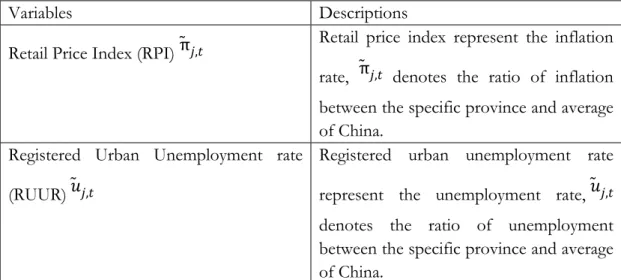
To ensure that all data are accurate in the thesis, data collected from the database of the National Bureau of Statistics of China (data.stats.gov.cn) and the statistical Yearbook. The data used in this section includes: annual Retail Price Index (RPI) to represent the inflation rate; annual Registered Urban Unemployment Rate (RUUR) to represent the unemployment rate. To ensure data integrity, time period is from 2000 to 2013, because some data are missing before 2000. I select 30 provinces without Tibet because of data missing in some time period.
Table 3.2: Variables and descriptions
Variables Descriptions
Retail Price Index (RPI) ̃π𝑗,𝑡 Retail price index represent the inflation
rate, ̃π𝑗,𝑡 denotes the ratio of inflation
between the specific province and average of China.
Registered Urban Unemployment rate (RUUR) ̃𝑢𝑗,𝑡
Registered urban unemployment rate represent the unemployment rate, ̃𝑢𝑗,𝑡
denotes the ratio of unemployment between the specific province and average of China.
3.3 Empirical investigation
Table 3.3: Descriptive Statistics for ̃π𝑗,𝑡 and ̃𝑢𝑗,𝑡
̃π𝑗,𝑡 Coefficient of Inflation ̃𝑢𝑗,𝑡Coefficient of unemployment Observations 420 420 Mean 0.984526112 0.973052972 Median 0.981818182 0.992472477 Std, Deviation 2.143320129 0.17810722 Variance 4.593821176 0.031722182 Range 35.45454545 1.321064916
Maximum 23.63636364 1.565675274
Minimum -11.81818182 0.244610358
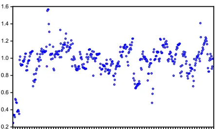
Based on selected data, table 3.3 illustrates descriptive statistics for ̃π𝑗,𝑡 and ̃𝑢𝑗,𝑡. ̃π𝑗,𝑡
means the ratio of inflation between the specific province and average of China. ̃𝑢𝑗,𝑡
denotes the ratio of unemployment between the specific province and average of China. Figure 3.3.1 and Figure 3.3.2 are ‘dot plot’ graphs. If the ratio is larger than 1, then the specific province has a larger inflation or unemployment rate than average; on the contrary, if ratio smaller than 1, average of China is larger than the specific province. The horizontal axis represents the coefficient in various provinces 29) at different times
(1-13).
0.2 0.4 0.6 0.8 1.0 1.2 1.4 1.6 1 0 0 2 0 1 3 0 2 4 0 3 5 0 4 6 0 5 7 0 6 8 0 7 9 0 8 1 0 0 9 1 1 1 0 1 2 1 1 1 3 1 2 1 4 1 3 1 6 0 0 1 7 0 1 1 8 0 2 1 9 0 3 2 0 0 4 2 1 0 5 2 2 0 6 2 3 0 7 2 4 0 8 2 5 0 9 2 6 1 0 2 7 1 1 2 8 1 2 2 9 1 3 RUUR
Figure 3.3.2: ̃𝑢𝑗,𝑡aggregated by province along the horizontal axis
In Figure 3.3.1, a few ‘dots’ are far away from the main group of other ‘dots’. As assumed before, the ratio of provincial inflation and the average inflation in China represents their relationship of one period, if a dot is scattered away from other dots. It means in this time period, the ratio of specific provincial inflation and average of China will be larger than others. For example, table 3.3 shows the maximum value of ̃π𝑗,𝑡 is
23.64, this maximum value comes from 2003 in Tianjin. In 2003, the local retail price index of Tianjin was -2.6%, which is not extremely high, while the annual weighted IUCP was only -0.11%. Compared with figure 3.3.1, Figure 3.3.2 for unemployment is not easy to observe data onto unemployment rate, because dots are too scattered. Remarkably, Figure 3.3.1 and Figure 3.3.2 have different scale on vertical axis, so it looks like the latter dots are more scattered, but in fact the former one are very scattered as well, because of the large scale. For the unemployment ratio, we can recognize that it is varying during this time period. But all the ratios are low, a majority of provinces are around 1.
4 Empirical Results
Table 4.1 demonstrates the results for three possibilities: 1) Equation 3.1.5 which includes fixed effect of provinces, 2) Equation 3.1.6 which includes fixed effect of time periods,3) Equation 3.1.7 which includes fixed effect of provinces and fixed effect for time periods. Fixed effects model is to compare the differences between categories of each category of independent variables and with the specific category/categories among other variables from the interaction effect. The difference between random effects and
fixed effects model is: in the random effects model, error terms and explanatory variables are irrelevant; but the fixed effects model assumes that the error term and the explanatory variables are related. All these equations have been interpreted in the section of the empirical study.
̃π𝑗,𝑡= λ ‒ φ
(
̃𝑢𝑗,𝑡)
+ ω(
̃π𝑗,𝑡 ‒ 1)
+ α𝑗+ ε𝑗,𝑡 (3.1.5, Model 1)̃π𝑗,𝑡= λ ‒ φ
(
̃𝑢𝑗,𝑡)
+ ω(
̃π𝑗,𝑡 ‒ 1)
+ ρ𝑡+ ε𝑗,𝑡 (3.1.6, Model 2)̃π𝑗,𝑡= λ ‒ φ
(
̃𝑢𝑗,𝑡)
+ ω(
̃π𝑗,𝑡 ‒ 1)
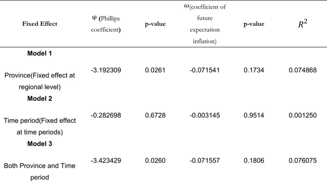
+ α𝑗+ ρ𝑡+ ε𝑗,𝑡 (3.1.7, Model 3)Table 4.1: Result of Panel Least Square with fixed effect
Fixed Effect φ (Phillips
coefficient) p-value ω(coefficient of future expectation inflation) p-value 𝑅2 Model 1 Province(Fixed effect at regional level) -3.192309 0.0261 -0.071541 0.1734 0.074868 Model 2
Time period(Fixed effect at time periods)
-0.282698 0.6728 -0.003145 0.9514 0.001250
Model 3
Both Province and Time period
-3.423429 0.0260 -0.071557 0.1806 0.076075
Value of φ denotes Phillips coefficient for each model, ω is the coefficient on future
expectation of inflation. The model 1 and model 3 have significant Phillips coefficients at 5 percent level. But the Phillips coefficient is insignificant for the model 2. All these three models have an insignificant coefficient of future expectation ω at 5 percent level.
Here, I need to consider the essential differences among these models. Model 1 is tested and to allow for provincial specific fixed effects, especially to find large differences in the natural unemployment rate between the provinces. Model 2 contains fixed effect of time periods, it is possible to include additional fixed effects for time periods. However, if the model includes such an effect, then we should suppose that the provincial specific effects vary with time. However, there is no evidence support such a theory, so time is an
invariant factor. Model 3 contains specific fixed effects of both provincial and time period. Hence, the model 1 is the most applicable model.
According purpose of this paper, empirical study focuses on the analysis of two kinds of relationships: the provincial and national differences; the relationship between inflation and unemployment. Thus, the Model 1 with fixed effect at the regional level is an available model.
The above method represents the basic Phillips curve. Since China's economic reform is still underway, perhaps the original Phillips curves is not completely satisfied with the case of China. Hence, I will use different Phillips curve models in the rest of this section, to adjust the existing three models, and analyze the results.
The modified Phillips curves is basing on ‘Okun’s Law (Graeme 2011), it includes the output gap of GDP instead of the unemployment rate. Although annual Registered Urban Unemployment Rate (RUUR) data is accurate, but there may be unregistered unemployed population, so I select the output gap of GDP as the independent variable of modified Phillips curves. To establish an output gap, here I select Hodrick-Prescott Filter to estimate the output gap of the GDP growth rate.
The Hodrick-Prescott Filter (HP Filter) is an instrument that used in real business cycle theory. It is used to remove the cyclical component of a time series from raw data and obtain a smoothed-curve representation of a time series, which is more sensitive to long-term than short-long-term fluctuations (Robert 1997). HP filter also applied for some purposes, such as estimation of the output gap (Assenmacher 2008). In this subsection, HP filter is applied for estimating the output gap
Basing on the first model of the expectations-augmented Phillips curve, a modified Phillips Curves model uses the output gap of GDP to replace the unemployment rate. Ratio of unemployment rate ̃𝑢𝑗,𝑡 can be replaced by the ratio of GDP gap ̃δ𝑗,𝑡. Equation
(3.1.1) can be rewritten as:
π𝑗,𝑡= λ + θ
(
𝑔𝑗,𝑡‒ 𝑔𝑗,𝑡∗)
+ ω(
π𝑗,𝑡 ‒ 2)
(4.1)𝑔𝑗,𝑡 is the output gap of provincial GDP at time period t, 𝑔𝑗,𝑡∗ represents the natural rate of output gap, θ denotes the coefficient of the Phillips curve, ω is the coefficient of future expectation of inflation
𝑔𝑎𝑣𝑒,𝑡 is the average of the output gap of provincial GDP. π𝑗,𝑡 π𝑎𝑣𝑒,𝑡= λ + θ
(
δ𝑗,𝑡 δ𝑎𝑣𝑒,𝑡)
+ ω(
π𝑗,𝑡 ‒ 2 π𝑎𝑣𝑒,𝑡 ‒ 2)
+ α𝑗+ ε𝑗,𝑡 (4.3)Equation (4.3) is merged from (4.1) and (4.2). λ is the intercept, δ𝑗,𝑡 is the output gap of
provincial GDP at time period t, δ𝑎𝑣𝑒,𝑡 denotes the average of the output gap of
provincial GDP. δ𝑗,𝑡
δ𝑎𝑣𝑒,𝑡 represents the output gap of GDP for a specific province 𝑗 in time period 𝑡 divided into the average output gap of China δ𝑎𝑣𝑒, 𝑡. θ is a positive Phillips
coefficient, to test whether two Phillips coefficients are different. If Phillips coefficients is different, θ will be different from 1. This means the provincial inflation is not 100% sensitive to the average of China to the changes of output gap of GDP.
π𝑗,𝑡 ‒ 2
π𝑎𝑣𝑒,𝑡 ‒ 2 is the variable of future expectation of inflation. ε𝑗,𝑡 is the error term. For the natural rate of
output gap, it is incorporated into specific fixed effectsα𝑗.
̃π𝑗,𝑡= λ + θ
(
δ𝑗,𝑡̃)
+ ω(
̃π𝑗,𝑡 ‒ 2)
+ α𝑗+ ε𝑗,𝑡 (4.4)Equation 4.4 is a simplified equation 4.3, it assumes δ𝑗,𝑡̃ equal to
δ𝑗,𝑡
δ𝑎𝑣𝑒,𝑡, ̃π𝑗,𝑡 ‒ 2 equal to π𝑗,𝑡 ‒ 2
π𝑎𝑣𝑒,𝑡 ‒ 2, α𝑗 is the fixed effect of each province
Equation 41.6 contains a new parameter ρ𝑡 which denotes the fixed effects for different
time periods. If consider both fixed effects of time periods and fixed effect of a specific province, then an equation with both α𝑗 andρ𝑡 is written as:
̃π𝑗,𝑡= λ + θ
(
δ𝑗,𝑡̃)
+ ω(
̃π𝑗,𝑡 ‒ 2)
+ α𝑗+ ρ𝑡+ ε𝑗,𝑡 (4.6)For the natural rates of output gap, they are incorporating into specific fixed effects α𝑗.
ρ𝑡 denotes the fixed effects of different time periods. Unlike the original Phillips curves models, in the modified models, I set two lags for
(
̃π𝑗,𝑡 ‒ 2)
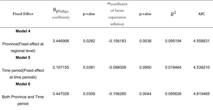
in the modified model. Table 4.2: Result of Panel Least Square with fixed effect (Output gap)Fixed Effect θ(Phillips
coefficient) p-value ω(coefficient of future expectation inflation) p-value 𝑅2 AIC Model 4 Province(Fixed effect at regional level) 3.446906 0.0282 -0.156183 0.0038 0.095194 4.558831 Model 5
Time period(Fixed effect at time periods)
2.107155 0.0381 -0.088009 0.0950 0.019464 4.539210
Model 6
Both Province and Time period
3.447026 0.0309 -0.156265 0.0044 0.095626 4.619465
Based on table 4.2, there are three sorts of modified models: 1) model 4 includes fixed effect of province time periods (equation 4.4); 2) model 5 is a fixed effect model of time periods (equation 4.5); 3) model 6 is a fixed effect model of province and time period (equation 4.6). Value of θ denotes Phillips coefficient for each model. ω is the coefficient
coefficients is positive. These three models have significant Phillips coefficients at 5 percent level. Except that, model 4 and model 6 have significant coefficients of future expectation ω at 5 percent level.
We can try to analyze the essential differences among these models. Model 4 is examined and to allow for provincial fixed effects, especially to find large differences in the natural output gap of GDP between the provinces. Model 5 includes fixed effect of time periods. Adding additional fixed effects for time periods is possible, while if the model includes such an effect, then we should suppose that the provincial specific effects vary with time. But there is no evidence support such a theory, so time period is invariant. Model 6 contains specific fixed effects of both provincial and time period.As I mentioned, θ is the coefficient to test whether the provincial Phillips coefficient and average Phillips coefficient are different. If the Phillips coefficient is different,
θ𝑗
θ𝑎𝑣𝑒 will be different from 1, provincial inflation is not equally sensitive to the average of China to the changes of GDP output gap. Therefore, the modified Phillips coefficient of 30 provinces is not alike the China’s average level. Provinces are more sensitive to changes of GDP output gap than the average of China.
In general, the results mean: when one unit of output gap ratio (δ𝑗,𝑡̃ ) increased, the
inflation rate ratio ( ̃π𝑗,𝑡) rose 3.92 units. Furthermore, ( ̃π𝑗,𝑡) is significantly different from
one. It means when the value of the output gap ratio (δ𝑗,𝑡̃ ) increase, the value of the
inflation rate ratio (̃π𝑗,𝑡) will be raised as well. But the difference in inflation between
provinces and average of China could be increase or decrease. It depends on the value of ̃π𝑗,𝑡, if the value is below 1. Rising (δ𝑗,𝑡̃
) pulls provinces to close to the average of China. For the coefficient ω, it represents how the past inflation ratio (two time periods ago) affects the current inflation ratio. When the ratio
(
̃π𝑗,𝑡 ‒ 2)
increased to one unit, thecurrent inflation ratio ̃π𝑗,𝑡 rose -0.15. If the value of ̃π𝑗,𝑡, is above 1, the difference
between provinces and average of China in the inflation rate at the current period will become smaller after two years, in other words they converge slightly.
Next step, to explain the provinces separately with the average of China, table 4.3 illustrates the result of each province specific model by simple linear least square model with time series data set.
θ p-value ω p-value 𝑅2 Beijing 14.31133 0.1866 -0.187313 0.5606 0.191761 Tianjin -67.21325 0.2553 -0.204932 0.5376 0.149213 Hebei -9.439866 0.2320 -0.193441 0.5760 0.154670 Shanxi(1)1 -5.354009 0.2107 -0.026303 0.9300 0.167953 InnerMongolia 1.266333 0.5960 0.003018 0.9925 0.035046 Liaoning -6.638588 0.8671 -0.185988 0.5897 0.042499 Jilin 19.44729 0.1941 0.030838 0.9198 0.200832 Heilongjiang 46.87221 0.0617 -0.614751 0.0011 0.738563 Shanghai 8.676196 0.1761 -0.272743 0.4140 0.203523 Jiangsu 1.198068 0.5044 -0.056103 0.8639 0.051004 Zhejiang 1.907155 0.2547 0.378465 0.1795 0.351915 Anhui 23.10550 0.1860 -0.170999 0.5954 0.188137 Fujian -22.89140 0.2179 -0.010256 0.9746 0.170343 Jiangxi 17.11790 0.0033 -0.574857 0.0028 0.765732 Shandong -3.241675 0.3870 0.058864 0.8605 0.106783 Henan -36.21281 0.5019 -0.202782 0.5607 0.069593 Hubei 22.88344 0.1527 -0.443784 0.1296 0.339058 Hunan 16.79920 0.1365 -0.528838 0.0835 0.366778 Guangdong -0.927454 0.6825 -0.427851 0.1869 0.184809 Guangxi 5.709999 0.2980 -0.493780 0.0611 0.390514 Hainan 28.74201 0.0837 -0.502116 0.0592 0.437017 Chongqing -2.036615 0.6132 -0.402828 0.2091 0.174808 Sichuan 1.335113 0.7022 0.259498 0.3241 0.148541 Guizhou 0.962091 0.5840 -0.471250 0.1101 0.269775 Yunnan 0.479559 0.7430 0.103777 0.7575 0.016151 Shanxi(2) 18.14900 0.2074 -0.067008 0.8333 0.170313 Gansu 7.971085 0.3309 0.023121 0.9474 0.113226 Qinghai 12.30848 0.7281 -0.047750 0.8928 0.014512 Ningxia -0.1576228 0.9426 -0.409038 0.2103 0.175022 Xinjiang -0.618629 0.7831 -0.618629 0.0100 0.540315
θ is the Phillips coefficient and ω is the expectations coefficient. Heteroscedasticity can be tested for Whites heteroscedastic test of each province (Appendix B). All the heteroscedastic provinces have been underlined in table 4.3.
Results of provincial specific regression show provinces and the average of China is different. Based on Table 4.3, there are only three provinces have acceptable P value which is smaller than 0.05. Also, each province has their own value of R2. Some province
like Jiangxi which can be explained by modified Phillips curve, because it has a small P value (0.0033). But for most of the other province, they do not have a small P value
which means they are insignificant. In general, it means for most of the provinces, a linear least square Phillips curve model with time series cannot perfectly interprets the inflation situation of each province.
According to the results of empirical study, we can conclude following information. First, provinces do not have a Phillips coefficient which is equal to the average of China, each specific province has different Phillips coefficients. Second, some provinces have similar sensitive to inflation to changes in GDP output gap as the average of China, but other provinces are not. Last but not least, although the fixed effect model of Philips curves at regional level is available to the case of China, there may be other economic factors which influence on inflation.
5 Conclusions
The main purpose of this thesis consists of investigating whether changes in unemployment for province affect the inflation rate for similar way as the average of China. In addition, the thesis test if the provincial inflation rate is convergent with average national inflation from 2000 to 2013. Basing on the theory original Phillips curves model, model 1 is the most applicable models. Model 1 is tested to allow for provincial specific fixed effects, especially to find large differences in the natural unemployment rate between the provinces. Based on the theory of ‘Okun’s Law, output gap replaced unemployment to adjust a modified Phillips curve model. In this case, model 4 is the most applicable models. It is tested to allow for provincial specific fixed effects, especially to find large differences in the natural output gap of GDP between the provinces. In the empirical study, both original Phillips curves and modified Phillips curves are appropriate if and only if fixed effect at regional level. When the output gap ratio increased to one unit, the inflation rate ratio would rise by more than one unit. Furthermore, ( ̃π𝑗,𝑡) is significantly different from one. When the ratio of past inflation
ratio (two time periods ago) increases to one unit, the current inflation ratio slightly decreased.
Reconsider the China’s economic situation. Compared to the national level, each province faces more sensitive inflation shock. It means changing into provincial GDP output gap impact on provincial inflation is larger than the national level. Inflation rate fluctuating with economic growth, while the inflation rates are different for each province due to specific own facts. Each province has their own economic development plan, since local officials have controlled regional economic policies, which mean these officials could design economic projects. Hence Changes in GDP output gap influence the provincial inflation rate is divergent with national inflation.
The final conclusion. In general, changing into GDP output gap of province affects the inflation rate different to the average of China, the provincial inflation rate divergent to national inflation level. For each province, economic disparities cannot be ignored. The Phillips curve model is applicable to the case of China. While there may be other factors affect the inflation.
This article has a few shortcomings. In essence inflation is a monetary phenomenon, to fully explain the inflation we must consider for money supply and national monetary policy and other factors. But this article is not an endogenous mechanisms of investigation into inflation, it aims to the discovery, whether the provincial inflation rate is convergent with national inflation by Phillips curve theory. Since Phillips curve is not fully appropriate for China, further research may start from other factors which affect inflation.
References
Anderson, James E. and Eric van Wincoop, (2003) ‘Gravity with Gravitas: A Solution to the Border Puzzle’American Economic Review 93 P 170–92.
Assenmacher-Wesche K, Gerlach S (2008) ‘Money growth, output gaps and inflation at low and high frequency: spectral estimates for Switzerland. J Econ Dyn Control 32:411– 435
Besley, T. A, Case, (1995). ‘Incumbent behavior: vote-seeking, tax-setting, and Yardstick competition’. American Economic Review 85,P 25-45.
Byström, Hans N.E. Olofsdotter, Karin. Söderström, Lars. (2005)‘Is China an optimum currency area?’Journal of Asian Economics 16 (2005) P 612–634
Cao, Tinggui. (2001). ‘The People’s Bank of China and its Monetary Policy’ Paper No. 14 Dornbusch, R.Startz, R. Fischer, S. (2008) ‘Macroeconomics’,McGraw-Hill/Irwin
Ching, Yi Lin. Wang, Chun (2013). ‘Forecasting China's inflation in a data-rich environment’. ‘Applied Economics’, Vol 45, P3049-3057
Graeme, Chamberlin (2011). ‘Okun’s Law revisited’. Economic& Labour Market Review. Feb 2011.
Gujarati, D. and Porter, D. (2009) ‘Basic Econometrics’ International Edition 2009, McGraw- Hill Education, Singapore
He, Qizhi. Fan, Conglai (2015) Forecasting inflation in China
Hodrick, Robert J. Prescott, Edward C (1997). ‘Postwar U.S. business cycles: An empirical investigation’ 1-16
Li, Huaqun. (2011) ‘Economic Structure and Regional Disparity in China: Beyond the Kuznets Transition’ International Regional Science Review April 2011,Vol. 34,No. 2, P 157-190.
Li, Shantong. Hou, Yongzhi (2008) ‘China Coordinated Regional Development and Market Integration, Beijing: EconomicScience Press’
Lu, Ding. (2008) ‘China's regional income disparity. An alternative way to think of the sources and causes’.Economics of Transition Volume 16(1) 2008, P 31-58
Lu, Meng. Milner, Chris. Yu Zhihong. (2012). ‘Regional Heterogeneity and China's Trade: Sufficient Lumpiness or Not?’Review of International Economics, 20(2) P 415-429
Mongelli, F.P. (2005) ‘What is European Economic and Monetary Union Telling us About the Properties of Optimum Currency Areas?’ Journal of Common Market Structures, Vol. 43, No. 3, P. 607-635.
Mundell, R. A. (1961). ‘A theory of optimum currency areas. American Economic Review’, 51, 657–665.
Nilsson, Anders (2011). ‘Divergent Inflation in Euroland, A Phillips Curve approach to the
EMU-12’
Penelop B, Prime. (2002) ‘China joins the WTO: How, Why and What now?’ Published in Business Economics, vol. XXXVII, No. 2 (April, 2002), P.26-32.
Phillips, A.W. (1958) ‘The Relationship between Unemployment and the Rate of Change ofMoney Wage Rates in the United Kingdom, 1861-1957’ Economica,Vol. 25, No. 100, P 283-299.
Tavlas, G. S. (1993). The ‘New’ theory of optimum currency areas. The World Economy, 16, 663–685.
Xu, C.(2011). ‘The fundamental institutions of China's reforms anddevelopment’.
Journalof EconomicLiterature49, P 1076-1151.
Xu, Zhenhui. Fan, Jianyong. (2012)‘China's Rehional Trade and Domestic Market Integrations’Review of International Economics 20(5), P 1052-1069
Yu, J. Zhou, L. Zhu, G (2014).‘Strategic Interaction in Political Competition: Evidence from Spatial Effect across Chinese Cities’
Zhang, Fei. Xu, Li Da. Tang, Bingyong. (1999) ‘Forecasting regional income inequality in China’European Journal of Operational Research 124 (2000) P 243-254
Zhu, Guobin. (2012). ‘The composite state of China under “one contry, Multiple systems”: Theoretical construction and methodological considerations’. I.CON (2012) VOL. 10. No. 1, 272-297
Internet database
data.stats.gov.cn (2015), Retail Price Index (PRI), Registered Urban Unemployment Rate (RUUR), URL: http://data.stats.gov.cn/index
China Labor Statistical Yearbook (1999-2014)
Appendix A
Unit root test for variables
Cross-Method Statistic Prob.** sections Obs
Null: Unit root (assumes common unit root process)
Levin, Lin & Chu t* -2.52694 0.0058 60 712 Null: Unit root (assumes individual unit root process)
Im, Pesaran and Shin W-stat -8.06057 0.0000 60 712 ADF - Fisher Chi-square 364.491 0.0000 60 712 PP - Fisher Chi-square 346.633 0.0000 60 780
P value smaller than 0.05, reject null hypothesis, this is No unit root
Appendix B
Correlated Random Effects - Hausman Test
Test Summary
Chi-Sq.
Statistic Chi-Sq. d.f. Prob.
Cross-section random 24.517323 2 0.0000
Hausman test is used to test whether a model of fixed effect (FEM) or random effect (REM) is appropriate. The null hypothesis: FEM and REM do not differ significantly. If the hypothesis is rejected, it means FEM is more suitable. Since the Prob value is 0, we can reject the hypothesis, then FEM is better.
Appendix C
Diagnostic tests for table 4.43 heteroscedasticity by Whites test If both P value smaller than 5%, there is a heteroscedasticity. Beijing F-statistic Obs*R-squared 2.122985 7.666547 Prob. F(5,6) Prob. Chi-Square(5) 0.1931 0.1756 Tianjin F-statistic Obs*R-squared 1.051411 5.604010 Prob. F(5,6) Prob. Chi-Square(5) 0.4671 0.3467 Hebei F-statistic Obs*R-squared 1.185635 5.963872 Prob. F(5,6) Prob. Chi-Square(5) 0.4141 0.3098 Shanxi(山) F-statistic Obs*R-squared 2.067607 7.593106 Prob. F(5,6) Prob. Chi-Square(5) 0.2012 0.1801 Inner Mongolia F-statistic Obs*R-squared 4.022442 9.242669 Prob. F(5,6) Prob. Chi-Square(5) 0.0600 0.0998 Liaoning F-statistic Obs*R-squared 0.180912 1.572111 Prob. F(5,6) Prob. Chi-Square(5) 0.9598 0.9046 0.7050 Jilin F-statistic Obs*R-squared 211.0089 16.33994 Prob. F(5,6) Prob. Chi-Square(5) 0.0000 0.0357 Heilongjiang F-statistic Obs*R-squared 12.72068 10.54879 Prob. F(5,6) Prob. Chi-Square(5) 0.0025 0.0321 Shanghai F-statistic Obs*R-squared 0.632540 4.142054 Prob. F(5,6) Prob. Chi-Square(5) 0.6841 0.5292 Jiangsu F-statistic Obs*R-squared 1.483753 6.634379 Prob. F(5,6) Prob. Chi-Square(5) 0.3199 0.2493 Zhejiang F-statistic Obs*R-squared 27.38449 11.49623 Prob. F(5,6) Prob. Chi-Square(5) 0.0005 0.0390 Anhui F-statistic Obs*R-squared 716.2528 11.97993 Prob. F(5,6) Prob. Chi-Square(5) 0.0000 0.0424 Fujian
F-statistic Obs*R-squared 11.50005 10.86615 Prob. F(5,6) Prob. Chi-Square(5) 0.0050 0.0541 Jiangxi F-statistic Obs*R-squared 1.369110 6.394946 Prob. F(5,6) Prob. Chi-Square(5) 0.3527 0.2697 Shandong F-statistic Obs*R-squared 23.58479 11.41900 Prob. F(5,6) Prob. Chi-Square(5) 0.0007 0.0437 Henan F-statistic Obs*R-squared 0.660974 4.262116 Prob. F(5,6) Prob. Chi-Square(5) 0.6669 0.5123 Hubei F-statistic Obs*R-squared 35.86452 11.61149 Prob. F(5,6) Prob. Chi-Square(5) 0.0002 0.0405 Hunan F-statistic Obs*R-squared 7.450623 10.33538 Prob. F(5,6) Prob. Chi-Square(5) 0.0149 0.0663 Guangdong F-statistic Obs*R-squared 0.325994 2.563526 Prob. F(5,6) Prob. Chi-Square(5) 0.8804 0.7669 Guangxi F-statistic Obs*R-squared 5.292312 9,781992 Prob. F(5,6) Prob. Chi-Square(5) 0.0331 0.0817 Hainan F-statistic Obs*R-squared 459.3443 11.96873 Prob. F(5,6) Prob. Chi-Square(5) 0.0000 0.0352 Chongqing F-statistic Obs*R-squared 0.348414 2.700160 Prob. F(5,6) Prob. Chi-Square(5) 0.8663 07461 Sichuan F-statistic Obs*R-squared 1.312009 6.267536 Prob. F(5,6) Prob. Chi-Square(5) 0.3706 0.2811 Guizhou F-statistic Obs*R-squared 0.178774 1.555938 Prob. F(5,6) Prob. Chi-Square(5) 0.9607 0.9065 Yunnan F-statistic Obs*R-squared 0.500440 3.531601 Prob. F(5,6) Prob. Chi-Square(5) 0.7677 0.6186 Shanxi(陕) F-statistic Obs*R-squared 1.041756 5.576464 Prob. F(5,6) Prob. Chi-Square(5) 0.4712 0.3496 Gansu F-statistic 0.333230 Prob. F(5,6) 0.8759
Obs*R-squared 2.608064 Prob. Chi-Square(5) 0.7601 Qinghai F-statistic Obs*R-squared 0.625149 4.110232 Prob. F(5,6) Prob. Chi-Square(5) 0.6886 0.5337 Ningxia F-statistic Obs*R-squared 3.919187 9.187053 Prob. F(5,6) Prob. Chi-Square(5) 0.0633 0.1018 Xinjiang F-statistic Obs*R-squared 6.953730 10.23394 Prob. F(5,6) Prob. Chi-Square(5) 0.0176 0.0689