THESIS
ALTERNATE BAR DYNAMICS IN RESPONSE TO INCREASES AND DECREASES OF SEDIMENT SUPPLY
Submitted by Andrew Bankert
Department of Civil and Environmental Engineering
In partial fulfillment of the requirements For the Degree of Master of Science
Colorado State University Fort Collins, Colorado
Fall 2016
Master’s Committee:
Advisor: Peter Nelson Brian Bledsoe
Copyright by Andrew Robert Bankert 2016 All Rights Reserved
ii ABSTRACT
ALTERNATE BAR DYNAMICS IN RESPONSE TO INCREASES AND DECREASES OF SEDIMENT SUPPLY
Gravel-bed rivers can accommodate changes in sediment supply by adjusting their bed topography and grain size in both the downstream and cross-stream directions. Under high-supply aggradational conditions, this can result in spatially non-uniform stratigraphic patterns, and the morphodynamic influence of heterogeneous stratigraphy during subsequent
degradational periods is poorly understood. We conducted an experiment in an 18.3 m long, 1.2 m wide straight rectangular channel where we developed alternate bars in a gravel-sand mixture under constant discharge and sediment supply then developed stratigraphy over existing bars through aggradation with two supply increases. The supply was then reduced back to the initial supply rate, causing degradation through that self-formed stratigraphy. We collected stratigraphic samples and made frequent measurements of the bed topography and flow depth, which were used with a two-dimensional hydrodynamic model to characterize flow conditions throughout the experiment. Migrating alternate bars stabilized during the first equilibrium phase creating bed surface sorting patterns of coarse bar tops and fine pools. During the first supply increase the bars remained stable as the pools aggraded. During the second supply increase the pools aggraded further, causing the boundary shear stress over the bar tops to increase until the bars gained the capacity to migrate and eventually stabilize in new locations. As aggradation occurred, the original sediment sorting patterns were preserved in the subsurface. During the degradational phase, the pools experienced incision and the bars eroded laterally, but this lateral erosion ceased when coarse sediment previously deposited during the bar-building phase became
iii
exposed. Our results suggest that if a sediment supply increase is capable of filling the pools it can cause stable bars to migrate and the bed to be reworked. Our findings also show that heterogeneous stratigraphy can play an important role in determining whether bars persist or disappear after a sediment supply reduction.
iv TABLE OF CONTENTS ABSTRACT ... ii CHAPTER 1: INTRODUCTION ... 1 CHAPTER 2: METHODS ... 5 Experimental Setup ... 5 Measurements... 7 CHAPTER 3: RESULTS ... 14 Bed Topography ... 14 Bedload... 20
Bed Surface Grain Size ... 20
Stratigraphy ... 22
Hydraulic Conditions ... 25
CHAPTER 4: DISCUSSION ... 29
Bar response to changes in sediment supply ... 29
Dynamic stratigraphy and critical shear stress ... 31
CHAPTER 5: CONCLUSION ... 35
1
CHAPTER 1: INTRODUCTION
Introduction
Sediment supply is widely recognized to be an important control on river channel morphology (e.g., Schumm, 1985; Buffington and Montgomery, 1997; Church 2006). Rivers adjust their slope and bed surface sediment grain size distribution to accommodate the upstream supply of sediment and water (e.g., Gilbert, 1877; Mackin, 1948; Lane, 1955; Hack, 1960, 1975; Knighton, 1998; Parker, 2007). Experiments have shown that gravel-bed rivers develop an armored surface, with less bed surface grain-size heterogeneity, when sediment supply is reduced (Dietrich et al., 1989; Nelson et al., 2009), and theoretical analyses have suggested that the grain size distribution of river bed material reflects that of the sediment supplied from adjacent
hillslopes (Sklar et al., 2006). When pulses of sediment are introduced to a river, as may occur after wildfire, from a landslide, or following dam removal or gravel augmentation, theory and experiments have shown that these pulses can evolve through dispersion, translation, or a combination of both, depending on flow characteristics, characteristics of the sediment pulse, and the extent to which channel width varies downstream of the pulse location (e.g., Lisle et al., 1997; Cui et al., 2003; Sklar et al., 2009; Nelson et al., 2015).
Despite increasing attention on the morphodynamic effects of sediment supply, our understanding of how bars in rivers may respond to changes in sediment supply remains limited. Robust analytical theory provides a mechanistic explanation of how alternate bars freely form and migrate downstream as a result of an inherent instability of flow and sediment transport fields with small perturbations in bed topography (Blondeaux and Seminara, 1985; Colombini et al., 1987). Yet with few exceptions (e.g., Nelson et al., 2014) these theories assume that the
2
sediment supply is equal to the channel’s sediment transport capacity, and they are unable to account for supply disequilibrium.
Flume experiments have provided valuable quantitative information on the relation between sediment supply and the dynamics of alternate bars. In general, these experiments have implemented either a supply increase or a supply decrease, but not both (but see Pryor et al., 2011). In a recirculating flume experiment, Podolak and Wilcock (2013) developed alternate bars and then augmented the sediment resupply upstream so that the sediment transport rate increased by a factor of 3. They observed the formation and migration of short-wavelength transient bars over the existing stationary alternate bars, reworking the bed until new stable bars eventually formed at positions near where bars had formed prior to the supply increase. As a tendency toward stable, nonmigrating bars have been observed in many experiments (e.g., Ikeda, 1983; Lanzoni, 2000; Nelson et al., 2010; Crosato et al., 2012), it is possible that a supply increase threshold must be eclipsed in order to temporarily overwhelm the stable bar configuration and rework the bed.
Lisle et al. (1993) and Venditti et al. (2012) conducted experiments in which alternate bars were allowed to develop, and then the sediment supply was reduced. With decreasing supply, Lisle et al. (1993) observed a narrowing of the zone of active sediment transport and coarsening of the bar tops, which exhibited low particle submergence and high relative roughness. Channel incision through the pools then caused the bars to become inactive and emerge. Conversely, Venditti et al’s. (2012) experiments exhibited lower relative roughness, and when the sediment supply was reduced the alternate bars disappeared, by migrating out the flume or from progressive lateral erosion. They suggested that the difference in bar response to reduced supply; i.e., pool incision vs. lateral bar erosion, was due to the differences in relative roughness
3
between the experiments. In natural channels, Lisle et al. (2000) noted a pattern between
sediment supply and width of equal mobility that was comparable to the observations in Lisle et al.’s (1993) flume experiments where the decrease in sediment supply led to a narrowing of the zone of active sediment transport. Lisle et al. (2000) also concluded that coarse areas of channel beds “created during earlier stages of channel evolution remain inactive”, similar to the
conclusions of Pryor et al. (2011) where high supply conditions controlled future channel response.
Under conditions where channel aggradation is followed by degradation, a river will create and then consume its own stratigraphy, and we do not yet have a quantitative or predictive understanding of how this may affect bar dynamics. Straight channels with alternate bars tend to have coarse bars and fine pools (e.g., Mosley and Tindale, 1985; Kinerson, 1990; Lisle and Hilton, 1992; Lisle and Madej, 1992). Flume experiments (Nelson et al., 2010) and numerical modeling (Nelson et al., 2015) studies suggest that in this pattern of coarse bar tops and fine pools is the result of interactions between spatially-varying boundary shear stress and the selective nature of lateral (cross-stream) bedload transport. As bars develop and migrate during aggradational conditions, these surface sorting patterns may be stored as stratigraphy. During subsequent degradational periods, the stratigraphy becomes the bed surface, and the potentially abrupt grain-size transitions associated with this exhumation may lead to feedbacks on
morphodynamic evolution that are difficult to predict a priori, especially if the stratigraphic layers exhibit strong lateral or longitudinal spatial variation in grain size.
4
where τ is the dimensional boundary shear stress, ρ and ρs are the density of water and sediment,
respectively, g is gravitational acceleration, and D is a characteristic grain size such as the median grain size of the bed material. Sediment is considered mobile when the local
dimensionless shear stress exceeds a critical value, which is frequently characterized by the Shields curve (e.g., Shields, 1936; Buffington and Montgomery, 1997). During aggradation, changes in bed morphology can lead to changes in the spatial distribution of boundary shear stress and therefore bed mobility, and during degradation, exposure of underlying stratigraphy can change local values of τ* by changing D, which may have important consequences for
patterns of bed evolution. To our knowledge, the effects of subsurface grain sizes on alternate bar dynamics have not been studied.
To better understand how bar dynamics are affected by increases and decreases in
sediment supply, we conducted a flume experiment where we developed alternate bars, increased the sediment supply, and then decreased the sediment supply. Frequent measurements of bed topography and bed surface grain size, along with measurements of subsurface grain size during equilibrium conditions, provide insight on how bed surface and subsurface sorting patterns influence the location and evolution of alternate bars. Our findings show that spatial variations in critical shear stress play an important role in determining whether bars will persist or migrate during both aggradational and degradational periods.
5
CHAPTER 2: METHODS
Experimental Setup
Our experiments were conducted at the Colorado State University Engineering Research Center hydraulics laboratory in a 1.2 m wide, 18.3 m long, 0.76 m deep rectangular flume. The overall goal of the experiments was to investigate bar dynamics in response to a cycle of
aggradation and degradataion by first developing alternate bars in heterogeneous sediment under an equilibrium sediment supply, then increasing the sediment supply so that the bed would aggrade and develop stratigraphy, and then decreasing the sediment supply to the initial condition to induce degradation.
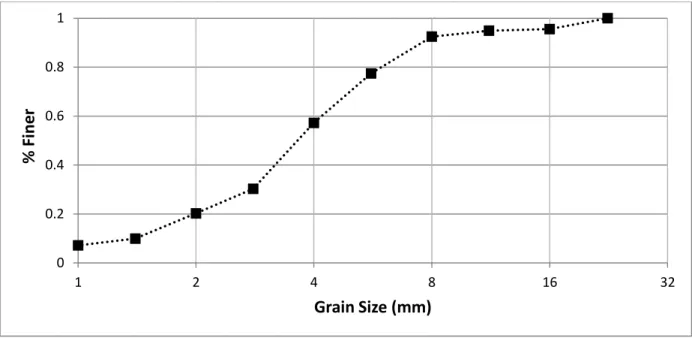
The sediment used throughout the experiment consisted of a lognormally distributed fine gravel to coarse sand mixture ranging from 1 to 22.5 mm with a median diameter (D50) of 3.64
mm, similar to the mixture used in the Venditti et al. (2012) experiments (Fig. 1). The flume was filled with 10-20 cm of sediment, which was mixed and screeded flat to an initial slope of
0.0095. Throughout the experiment, the discharge was held constant at 0.096 m3/s, which was set to keep the width to depth ratio at about 20 in order to promote the development of alternate bars.
6
Figure 1: Grain size distribution of the bulk sediment mixture used throughout experiment.
The downstream water surface elevation was maintained with an adjustable tailgate. A sediment weir at the end of the flume kept the downstream bed elevation constant, and concrete blocks and large cobbles placed in the bed at the upstream end of the flume prevented scour at the inlet. Only the downstream 15 m of the channel were analyzed to avoid entrance effects. A sediment trap captured bed load material that exited the flume. The trap was emptied every 0.5-3 hours, at which point the sediment was dried and weighed to determine the bed load transport rate exiting the flume. A subsample of the trapped sediment was then sieved to characterize the grain size distribution of the bed load material. The sample for sieving was pulled from several locations in the sediment trap to avoid bias associated with heterogeneous sediment transport.
An adjustable rate sediment feeder supplied sediment to the upstream end of the flume. The experiment was split into three phases, where in each phase we changed the sediment feed rate. Each phase of the experiment was run until the bed load transport rate exiting the flume and the grain size of the transported sediment matched the rate and grain size of the sediment feed.
0 0.2 0.4 0.6 0.8 1 1 2 4 8 16 32 % Fi n e r Grain Size (mm)
7
The equilibrium phase (Phase 1) fed a low supply (134 kg/h) for 53 hours as the channel formed stable alternate bars while reaching equilibrium. The aggradational phase (Phase 2) was split into two sediment supply increases. Phase 2.1 increased the sediment supply to 250 kg/hr for 37.75 hours, then the supply was raised to 331 kg/hr during Phase 2.2, which lasted 33.25 hours. The degradational phase (Phase 3) returned the sediment supply back to the initial supply of 134 kg/hr for 25 hours.
Measurements
The flume was run in 0.5- to 3-hour increments to allow for frequent measurements as well as sediment trap clearing. Each time the flume was restarted, the discharge was slowly increased from zero to 0.096 m3/s to minimize sediment transport associated with a rapid
increase in discharge. During Phases 2 and 3, water depths were measured with a tape measure at 0.61 m intervals along the channel centerline. During Phase 1, water depths were taken along the flume walls but these measurements were not accurate enough to be included in the results.
After each increment of run time, the flume was drained so that detailed measurements of bed topography and grain size could be collected. Bed topography was characterized using structure-from-motion (SfM), which involved taking photographs of an object or surface from many different angles, and then using software to align the images and produce a very dense 3-dimensional topographic point cloud. Morgan et al. (in review) have demonstrated that in laboratory applications, SfM techniques produce topographic datasets that are at least as accurate, and of higher resolution, than terrestrial laser scanning.
To facilitate SfM data collection and comparison of sequential topographic datasets, we affixed flat targets to the inner walls of the flume, with a spacing of approximately 0.6 m. The
8
coordinates of these targets were determined with a Leica ScanStation terrestrial laser scanner (TLS), and they were used to scale and register each topographic point cloud derived from SfM. Each time the flume was shut down, we collected two series of photographs of the flume bed and targets with an 18 megapixel Canon T3i DSLR camera with a fixed 24 mm lens. The camera was mounted to the center of a measurement cart mounted to horizontal rails on the flume walls. Photographs were taken in both the upstream and downstream directions, with the camera angled approximately 45 degrees below horizontal so that each photo captured the channel bed as well as the targets on the flume walls. Photographs were taken at 0.3 m intervals to ensure at least 70% overlap between each photo. Each series of photographs was processed in Agisoft Photoscan Professional, which produced three-dimensional topographic point clouds with an average point density of 4.27 points/cm2. Test SfM datasets of the flume collected prior to the experiments presented in this paper were compared with TLS scans using a cloud to mesh differencing (Cignoni and Rocchini, 1998), the mean error from the DEM generated using structure from motion was less than 1 mm, and 90% of the points showed less than a 2 mm difference.
Each SfM point cloud was interpolated onto a 1 cm x 1 cm digital elevation model (DEM) using a nearest neighbor algorithm. The grid was then trimmed to remove the walls as well as the upstream 3.3 m of the channel. The 1 cm x 1 cm elevation grid was used to generate longitudinal profiles of the mean elevation at each downstream grid cross-section. The average bed slope was computed by fitting a linear regression to these profiles. The slope was then used to create detrended elevation maps where the elevation of the average slope was subtracted from the elevation at each point. These detrended maps simplified the process of identifying the bars and pools during each run. Longitudinal descriptions of local topographic relief were also
9
calculated by subtracting the average of the five lowest elevations from the average of the five highest elevations at each cross section on the 1 cm x 1 cm grid. Pairs of grids collected at different times were differenced to characterize spatial patterns of erosion and deposition.
We characterized the bed surface grain size distribution using an automated image analysis procedure (Graham et al., 2005). We adopted this approach because we did not want to disturb the bed with surface sampling, and this technique has been used successfully to
characterize sorting and patchiness in previous gravel-bed flume experiments (Nelson et al., 2010, 2014). During each period when the flume was turned off, photographs for characterizing the local bed surface grain size distribution were collected at 84 locations on a 4 x 21 point grid. The points were spaced 0.305 m across the flume (between 0.15 and 1.07 m from the right wall) and 0.610 m in the streamwise direction (between 1.2 and 13.4 m from the downstream end of the flume). At each location a photograph was taken with the 18 megapixel Canon T3i DSLR with a 55 mm lens aimed orthogonal to the bed. The camera was mounted to a point gage on the mobile cart allowing each photograph to be taken from the same distance above the bed, so that each photo had the same resolution of 17 pixels/mm. Each photo was saved in RAW format and processed with Canon Digital Photo Professional 4.4 to remove lens distortion. The corrected photos were then processed using the automated image analysis method. For all analyses, the area-by-number grain-size distributions produced by the automated image analysis technique were converted to grid-by-number (or equivalently volume-by-weight) distributions using the voidless cube model (Kellerhals and Bray, 1976).
The Graham et al. (2005) method requires specification of several parameters, which are used to blur image noise and grain imperfections, enhance contrast between light and dark pixels, and determine which pixels are likely grain edges. We chose these parameters by performing
10
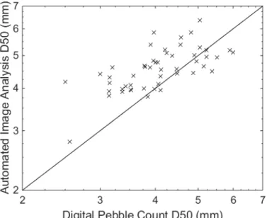
manual digital pebble counts on a subset of 50 bed photographs and comparing the results to the automated image analysis produced with a wide range of parameter combinations (Table 1). For the digital pebble counts, we brought the digital image into ArcGIS and overlaid onto it a 10 x 10 point grid. The semi-major axis of each particle onto which a grid point fell was drawn, and the length of each line was measured to develop a grid-by-number grain size distribution. The parameter values which produced the lowest overall error are given in Table 1, and using these values the average error between the median grain size from the automated image analysis and the digital pebble count methods was 10.3% (Fig. 2). Finer areas of the bed tend to be
overpredicted with the image analysis method, potentially due to the h-minima thresholding, as observed in Nelson et al. (2010). The autocorrelation method described by Warrick et al. (2007) and the wavelet method described by Buscombe (2013) were also compared against the manual digital pebble counts, but neither performed as well as the Graham et al. (2005) method.
11
Figure 2: Comparison of grain size estimates in digital pebble count vs. results from the automated image analysis.
Table 1: Values of parameters used in the automated image analysis. All combinations of the tested values were compared against digital pebble counts, and the values that produced the lowest error were used for all bed surface photo datasets.
Parameter Value Used Values Tested
Threshold 1 35 25, 30, 35, 40
Threshold 2 4 3, 4, 5
Disk Radius 7 5, 6, 7, 8
Median Filter 4 3, 4, 5
H-minima Threshold 1 0, 1, 2
At the end of each phase of the experiment, when equilibrium conditions had been reached, subsurface stratigraphy samples were taken at 6-8 locations in the flume bed. Because subsurface sampling is destructive to the bed, different locations were sampled after each experimental phase. Five locations spaced 3.05 m along the centerline, along with other
12
locations on bar tops and in pools, were sampled after each phase. Subsurface samples were collected using a 15 cm x 30 cm coring box similar to that described by Blom et al. (2003). At each location, the open-bottomed box was placed on the bed and hammered into the subsurface. Once the box was about 8 to 10 cm deep, a closing plate was hammered in from the top at a 45° angle, preserving the sediment core in the box and closing off the bottom. The box containing the sediment sample was then lifted vertically from the bed. The front wall was then lowered at 1 cm intervals and a cutting plate was inserted into the sediment horizontally to remove each 1-cm thick layer of sediment. Six layers were collected from each sample, and each layer was sieved and weighed to characterize the vertical subsurface grain size distribution. After sieving, each sample was replaced in the bed in an attempt to restore each sample site with a stratigraphy similar to what was removed in order to minimize the destructive effects of this sampling method.
Because shallow flows made it difficult to measure velocity in the flume, we
characterized the hydraulic conditions throughout the experiment by modeling the flow with the two-dimensional hydrodynamic model FastMECH (Flow and Sediment Transport and
Morphological Evolution of Channels), which is part of the free and open-source i-RIC
(International River Interface Cooperative) suite of models (Nelson et al., 2016; www.i-ric.org). FaSTMECH is fully described in Nelson and McDonald (1995), but in summary, it solves the full vertically averaged and Reynolds‐averaged momentum equations cast in a channel-fitted curvilinear orthogonal coordinate system as presented in Smith and McLean (1984). The model assumes steady, hydrostatic flow and it uses an isotropic eddy viscosity to account for
13
We used FaSTMECH to compute the flow depth, depth-averaged velocity, and boundary shear stress for most SfM topographic datasets we collected (a total of 60 flow calculations). The SfM DEM elevations were interpolated onto a Cartesian rectangular grid with computational nodes spaced 4.7 cm in the streamwise direction and 4.2 cm in the cross-stream direction. For all simulations the lateral eddy viscosity was set to 0.009 m2/s and the drying depth was set at 5 mm. The downstream stage and bed roughness were adjusted for each model simulation to maximize agreement between model-predicted and measured flow depths. The bed roughness drag
coefficient was spatially constant and took values between 0.075 and 0.095. The parameters were adjusted until the root mean square error between the measured and modeled water depths was within than 1 cm (Fig. 3).
Figure 3: Example of FaSTMECH water surface elevation (blue line) compared with measured values (blue dots) along with the bed elevation (black line) at Time = 83 h.
14
CHAPTER 3: RESULTS
Bed Topography
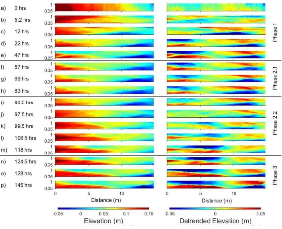
A subset of SfM derived DEMs that summarize the topographic evolution of the bed throughout the experiment are shown in Fig. 4 and 5. Figure 4 shows the elevations, both absolute and detrended, and Fig. 5 shows areas of aggradation and degradation throughout the experiment. The bed was initially flat with a slope of 0.0095 (Fig. 4a, Fig. 6d), but bars began forming quickly after the experiment began. Small, short bars rapidly moved down the channel before growing and slowing their migration rates. After 5.2 hours, a large bar-pool sequence had formed and was actively migrating down the channel at a rate of 1 m/hr (Fig. 4b). As this
sequence approached the downstream end of the channel, it began to stabilize and a second bar began to form upstream (Fig. 4c). As the bars stabilized after 22 hours, they became more defined as the channel degraded through the pools to decrease the slope (Fig. 5c and 5d). When the channel reached equilibrium during Phase 1 after 47 hours, the channel slope was 0.0057 (Fig. 6d) and the bed at the upstream end had degraded about 5 cm (Fig. 7).
15
Figure 4: A subset of SfM derived topographic DEMs collected during the experiment. The left map shows the actual elevation during selected runs, and the right map shows the detrended elevation with the slope removed. The horizontal lines between runs delineate the different phases. Flow was from left to right.
16
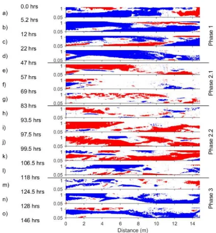
Figure 5: Areas of aggradation (red) and degradation (blue) of more than 1 cm between times bounding the left side of each map. The horizontal lines between runs delineate the different phases. Flow was from left to right.
17
Figure 6: Time series of (a) sediment feed rates and bed load transport rates of sediment exiting the flume, (b) flume-averaged median bed surface grain size, (c) median grain size of the
transported material collected in the downstream bedload trap, (d) mean bed slope, (e) mean flow depth along the channel centerline, (f) average topographic relief.
18
Figure 7: Longitudinal profiles of average bed elevation at each grid cross-section at the end of each phase of the experiment.
Increasing the sediment supply from 134 to 250 kg/h during Phase 2.1 caused the channel to become steeper, with lower cross-sectional relief, but the supply increase did not cause a complete reworking of the channel. The pools began to aggrade, but the elevation of the bar tops remained unchanged (Fig. 5e). During Phase 2.1, the overall topographic relief decreased by 26% (Fig. 6f) primarily because the elevation of the bottom of the pools rose by an average of 3.44 cm while the elevation of the bar tops aggraded just 0.34 cm. The aggradation of the pools enabled small amounts of lateral erosion in the bars (Fig. 5d). The average slope increased from 0.0057 to 0.0070 during Phase 2.1.
The second increase in sediment feed rate from 250 kg/h to 331 kg/h during Phase 2.2 led to more dramatic topographic changes. Shortly after the supply increase, short bars moved quickly through the pools (Fig. 4i), aggrading them to the point where the original bars were laterally eroded (Fig. 5h), bringing the bed surface close to planar (Fig. 4j). At 97.5 hours these short, fast-moving bars were migrating through the flume at rates greater than 9 m/hr. The bars quickly grew and slowed their migration rate until, by 99.5 hours, a larger bar-pool sequence
19
began to stabilize at a location about 2 meters downstream of the location of the stable bars present during Phases 1 and 2.1 (Fig. 4k, 4l). As the bars stabilized, the channel began degrading through the pools (Fig. 5k, 5l), causing the bar tops to emerge from the channel, until equilibrium was reached at 118 hours. During Phase 2.2, the average channel slope increased from 0.0070 to 0.0084 while the bars migrated through the channel over a planar bed at 103.5 h, then the slope decreased to 0.0069 while the bars stabilized (Fig. 6d). Overall, the entire flume bed aggraded an average of 3.5 cm during Phase 2.2 (Fig. 7).
During Phase 3, when the sediment supply was returned to the initial rate of 134 kg/h, the channel degraded through the pools while the bars underwent erosion only at the bar head and edge, making them more defined (Fig. 5m). Once this lateral erosion stopped, the bars became completely inactive. The upstream bar width decreased by 10 cm during the degradation phase. Since the degradation was almost exclusively limited to the pools, the elevation of the bar tops remained relatively unchanged while the elevation of the downstream pool decreased by 5 cm. During degradation, the channel slope initially decreased to 0.0051 before rebounding to 0.0060 as the channel approached equilibrium (Fig. 6d).
Despite the same sediment supply and discharge, the equilibrium bed topography at the end of Phase 1 differed from that at the end of Phase 3. The upstream bar at the end of Phase 3 was 2 meters further downstream and 2 meters longer than in Phase 1 (Fig. 4e and 4p), reflecting the conditions inherited when the bed was reworked during Phase 2.2. Figure 7 shows that the mean bed elevation at the end of Phase 3 was on average 1.35 cm higher than at the end of Phase 1, while the average channel slopes were roughly equal (0.0057 vs. 0.0060, Fig. 6d). The average topographic relief was similar at the end of Phases 1 and 3 (1.9 vs. 1.8 cm, Fig. 6f).
20 Bedload
Figures 6a and 6c show time series of sediment feed, sediment transport exiting the flume, and the median grain size of the transported sediment. When the supply rate was changed from one phase to the next, after a lag of between 8 and 13 hours the sediment transport rate out the end of the flume equilibrated to the feed rate (Fig. 6a), and throughout the experiment the median grain size of the transported sediment fluctuated around the median grain size of the bulk sediment supplied to the feeder (Fig. 6c). This shows that each phase of the experiment achieved equilibrium conditions.
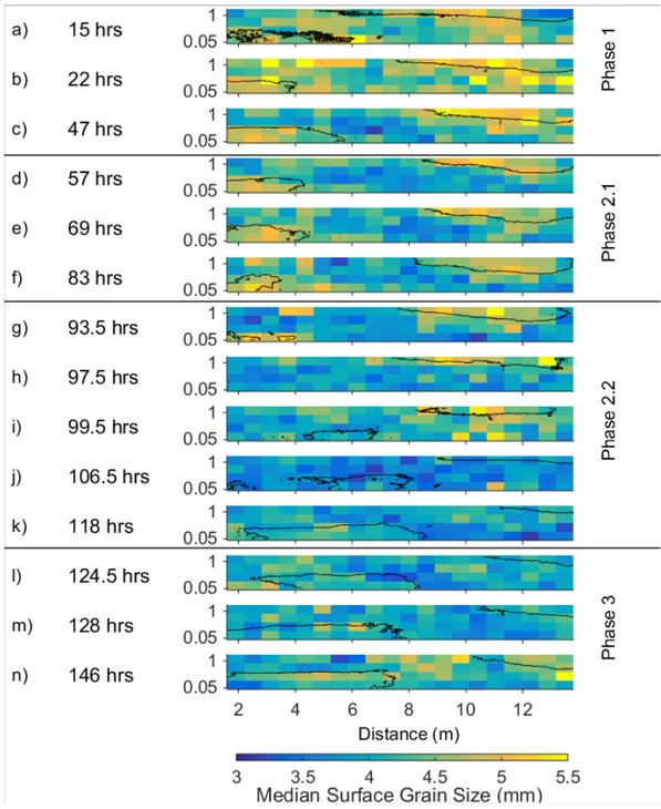
Bed Surface Grain Size
In general, the bed surface became finer as the supply increased and became coarser as the supply decreased (Fig. 6b). Shortly after the experiment began, bars began to form and the sorting pattern of coarse bar tops and fine pools typically observed in alternate bars in straight channels developed (Fig. 8). Throughout much of the experiment, the bar tops exhibited a
uniform coarse layer, while the pools consisted of a wide gradation of both fine grains and coarse grains, which may have rolled downhill off of the bars. A thin band of uniform fine sediment was often observed at the edge of the upstream bar, but the width was too small to be well documented through the automated image analysis. The bed surface D50 at the end of Phase 1
shows a distinct pattern with a coarser median grain size on the bar tops and a finer median grain size in the pools (Fig. 8c). These patterns were still distinct after Phase 2.1 (Fig. 8f), but during Phase 2.2 the mobile bars aggraded over the previous sorting patterns, and the bed surface developed a more uniform and finer grain size (Fig. 6b and 8j). The bed coarsened as the sediment supply decreased during the Phase 3, but since the bar tops had become inactive this adjustment mainly occurred in the pools resulting in less obvious bar-pool sorting patterns (Fig.
21
8n). The bed surface was not as coarse at the end of Phase 3 as it was at the end of Phase 1 even though the discharge and sediment supply conditions were the same for both phases (Fig. 6b).
Figure 8: A subset of median surface grain sizes collected through the automated image analysis process. Contour lines show the locations of bars greater than 2 cm above the mean longitudinal profile. Horizontal lines between runs delineate the different phases. Flow was from left to right.
22 Stratigraphy
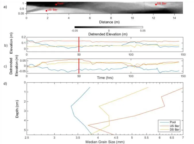
Figures 9 through 11 show vertical profiles of the median grain size from stratigraphy samples, along with time series of the elevation and detrended elevation at each sampling
location derived from the SfM topographic data. Despite the degradational nature of Phase 1, the grain size distribution 3 cm below the surface reflected the overall surface sorting pattern of coarse bar tops and fine pools that developed. This can be seen in the coarse grains 2.5 cm below the surface in both the upstream and downstream bars as well as the fine grains 2.5 cm below the pool in (Fig. 9d). Figure 9b shows that even though the overall tendency in the bed was to degrade during Phase 1, the bars underwent some aggradation before stabilizing. The coarse grains several centimeters into the subsurface were likely deposited during this local aggradation.
23
Figure 9: (a) Sampling locations of subsurface samples collected at the end of Phase 1; (b) time series of elevation at each sampling location; (c) time series of detrended elevation at each sampling location; (d) vertical profiles of median grain size of the subsurface samples. The vertical lines in (b) and (c) show the time at which the samples were collected.
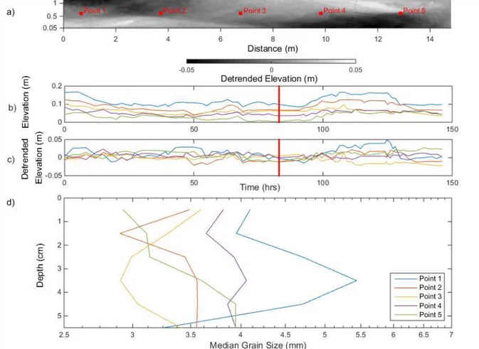
The most significant change during Phase 2.1 occurred when a finer layer of sediment buried a portion of the upstream bar. This is most noticeable at Point 1 in Fig. 10d where the sediment from 3-5 cm deep is noticeably coarser than the sediment closer to the surface. At the end of Phase 1, Point 1 had a relatively high detrended elevation of 0.0287 m, but by the end of Phase 2.1 its detrended elevation had declined to -0.0027 m (Fig. 10b), so the buried coarse grains likely reflect the coarse sediment that formed the bar top at Point 1 at the end of Phase 1. Points 2 and 3 aggraded slightly between the ends of Phase 1 and Phase 2.1 (Fig. 10b), and their subsurface samples exhibit a local minimum D50 between 1.5 and 3.5 cm below the surface,
24
likely fine pool sediment that was buried as the pools filled in with sediment during Phase 2.1. Subsurface samples collected from bars at the end of Phase 2.2 also exhibit coarse sediment 3 cm below the surface (Fig. 11d). Points 4 and 5 on the edge of the bar show coarse sediment at the surface with finer grains in the subsurface. Points 1 and 2, which lost the most elevation during the subsequent degradation in Phase 3 (Fig. 11b), had the finest grains 2.5 cm below the surface.
Figure 10: (a) Sampling locations of subsurface samples collected at the end of Phase 2.1; (b) time series of elevation at each sampling location; (c) time series of detrended elevation at each sampling location; (d) vertical profiles of median grain size of the subsurface samples. The vertical lines in (b) and (c) show the time at which the samples were collected.
25
Figure 11: (a) Sampling locations of subsurface samples collected at the end of Phase 2.2; (b) time series of elevation at each sampling location; (c) time series of detrended elevation at each sampling location; (d) vertical profiles of median grain size of the subsurface samples. The vertical lines in (b) and (c) show the time at which the samples were collected.
Hydraulic Conditions
The average flow depth shortly after the end of Phase 1 was 54 mm (Fig. 6e). As the slope increased during Phase 2.1 (Fig. 6d), the average flow depth decreased to 41 mm before rebounding to 52 mm (Fig. 6e). Phase 2.2 saw a similar response to increased supply with the average flow depth decreasing to 41 mm before rebounding to 45 mm (Fig. 6e). The shallower flow depths while the channel was responding to the change in sediment supply during each aggradation phase correspond to times where the surface grain size was finer than the equilibrium surface grain size. Like the surface grain size response, the average flow depth steadily approached the equilibrium flow depth of 58 mm during Phase 3. Unlike the flow depth,
26
the average bed slope decreased to a value below the equilibrium slope before rebounding during Phase 3 (Fig. 6d).
The average boundary shear stress over the entire channel, calculated as τ = ρghS, where
h and S are the measured depth and slope, is plotted in Fig. 12a. During each supply increase, there is a pattern of a decrease followed by a rebound of boundary shear stress, similar to what was observed in the flow depth. The lowest depth-slope product average shear stresses occurred during equilibrium in Phase 2.2, and the mean boundary stress gradually increased after the supply was reduced.
The model-predicted boundary shear stress field is spatially heterogeneous, with the highest shear stresses in the pools and low stresses over the bars (Fig. 13). Figure 12a presents time series of the flume-averaged boundary shear stress computed by the model, along with total stress estimates from both model-predicted average depths and water surface slopes, and the observed average water depths and bed slopes presented in Fig. 6. In general, there is good agreement between the depth-slope products computed from model output and from flume observations. The modeled depth-slope product was 15-20% higher than the channel averaged modeled shear stress during most runs, with a notable exception during Phase 2.2 when the channel was close to planar and the measured depth-slope product, the modeled depth-slope product, and the channel-averaged shear stress from FaSTMECH were similar. The modeled shear stress at the end of Phase 3 remained higher than that at the end of Phase 1 because the roughness in the model needed to be higher for the modeled flow depths to better match the measured flow depths.
27
The overall momentum extraction due to the presence of the bars is illustrated in Fig. 12b, where the ratio of the flume-average model-computed boundary shear stress to the depth-slope product computed with the flume-average modeled depth is shown. During Phases 1, 2.1, and 3, when bars are the dominant bed topography, the average boundary shear stress is about 70-80% of the depth-slope product, but during Phase 2.2 it at times is more than 90% of the depth-slope product.
Figure 12: (a) Shear stresses from numerical model, both depth-slope product and channel
average local shear stress, compared with measured depth-slope products throughout experiment. (b) Ratio of channel-averaged shear stress and depth-slope product from numerical model.
28
Figure 13: A subset of shear stress maps from the numerical model. Contour lines show the locations of bars greater than 2 cm above the mean longitudinal profile. Horizontal lines between runs delineate the different phases. Flow was from left to right.
29
CHAPTER 4: DISCUSSION
Bar response to changes in sediment supply
During the aggradation and degradation phases, our experiment exhibited dynamics that were similar to other studies in which the supply was either increased (i.e., Podolak and Wilcock, 2013) or decreased (i.e., Lisle et al., 1993; Venditti et al., 2012). The second supply increase in our experiment (Phase 2.2) resulted in the formation of small bars which migrated through the pools allowing for the erosion of the previously stable bars, ultimately leading to a complete reworking of the bed until new, stable bars formed. This response was similar to that described by Podolak and Wilcock (2013); however, the smaller mobile bars in our experiment neither decreased in size nor became incorporated into the larger bars. Instead, these smaller bars raised the pool bed to the point where the channel gained sufficient capacity to laterally erode the larger stationary bars as shown in Fig. 5h and 5i. As the previously stable and immobile bars eroded, the smaller bars grew laterally and slowed their migration rates, until they eventually grew into a new set of stationary bars (Fig. 4k through 4m).
The bed in our experiment only reworked itself during the second, higher, supply increase. During the first supply increase (Phase 2.1), the pools aggraded, which decreased the overall topographic relief (Fig. 6f) and allowed the flow depth and shear stress at the bar edges (Fig. 13c-f) to increase to a point where some coarse grains at the edges became entrained. The bars did undergo minor lateral erosion during Phase 2.1 (Fig. 5e) as the pools aggraded. This lateral erosion increased the width of high local shear stress (Fig. 13d-f), which likely increased the width of equal mobility as seen in Lisle et al.’s (1993) flume experiment and Lisle et al.’s (2000) field experiment, but it was insufficient to erode the entire bar. The additional
30
aggradation in the pools associated with the migratory bars during Phase 2.2 increased the shear stress over the bars even more (Fig. 13f-h), ultimately leading to the complete reworking of the bed, similar to the response in Podolak and Wilcock (2013). The different response of the bed between Phases 2.1 and 2.2 suggests that the bars will remain stable unless a sediment supply increase exceeds a threshold that produces sufficient pool filling to cause local shear stresses to become large enough to completely erode the bar edges, at which point the bed may be
reworked.
During the degradational phase (Phase 3), our channel responded to the reduced sediment supply with both incision in pools and lateral erosion of stable bars, essentially a combination of the responses to supply reduction reported by Lisle et al. (1993) and Venditti et al. (2012). Because the flow depth and shear stress over the bars were low enough to prevent local sediment transport during equilibrium stages, the main channel response to the supply decrease was incision through the pools. As this incision occurred, the shear stress at the edge of the bars became high enough to mobilize the coarse grains at the bar edge and erode the bars laterally, which widened the zone of active sediment transport. Lateral erosion did not continue until the bar disappeared (as in Venditti et al.’s (2012) experiments), but stopped after the bar had eroded about 10 cm laterally. Figure 14 shows the degradation of the pool as well as the lateral erosion of the bar at x = 4 m, the cross section with the highest relief. At 136 h, the lateral erosion
stopped and the bottom of the pool stabilized, suggesting that the lateral erosion may have ceased because the system approached a new equilibrium.
31
Figure 14: Degradation of a bar-pool cross stream during Phase 3 at x = 4 m. Dynamic stratigraphy and critical shear stress
In order to investigate the role that exhumation of heterogeneous bed stratigraphy may have played in the tradeoff between pool incision and lateral erosion shown in Fig. 14, we can use the rather high-frequency bed topography and bed surface grain size measurements to develop a simple stratigraphy model. This model initially discretized the vertical column of sediment underlying each automated image analysis grid location into a stack of 1 mm thick layers extending from an arbitrarily low bottom elevation up to the bed elevation, and it initially specified the D50 in each layer to be that of the bulk sediment mixture. Marching forward in time,
consecutive bed DEMs were used to compute the elevation change at each location between measurement times and to determine whether the bed had aggraded or degraded during that period. For each time step, the model assumes that the bed surface D50 estimated from the
32
automated image analysis technique extends 4 mm into the subsurface. If the bed aggraded locally more than 4 mm, then the median grain size between the new surface elevation and the old surface elevation is set at the new measured surface grain size and the rest of the stratigraphy remained the same as the previous time step. If the channel aggraded less than 4 mm or
degraded, the top 4 mm of the new surface elevation were replaced by the new measured grain size and the rest of the stratigraphy more than 4 mm below the new surface remained the same as in the previous time step. The vertical grain size profiles estimated with the simple model were compared against the subsurface samples collected after Phase 2.2 (chosen because the samples had the most heterogeneous stratigraphy) and were found to have a mean error of 10.3%. The model tended to predict the general pattern of coarse/fine layers well, but it usually under predicted the magnitude of change between layers. This discrepancy likely resulted from some combination of errors in the automated image analysis grain-size measurement, uncertainties in the subsurface measurements, and the model’s assumption that surface sediment was not reworked during aggradation.
Boundary shear stress over the bars, relative to the local critical shear stress (and
therefore the local bed surface grain size), is an important factor in determining the persistence of bars in natural channels (Lisle et al., 2000). The bars in our experiment likely responded based on the ratio of boundary shear stress, which changed as the pools eroded, to critical shear stress, which changed as subsurface grains became exposed. Figure 15 shows the vertical distribution of subsurface sediment D50 predicted by the simple stratigraphy model for two locations on the
upstream bar near x = 4 m depicted in Fig. 14 which showed different responses to the supply reduction. Figure 15l corresponds to y = 0.46 m, which was on a bar top that did not erode during Phase 3, and Fig. 15m corresponds to y = 0.76 m, which started Phase 3 on a bar but was
33
laterally eroded during the supply reduction. Both the model and the subsurface measurements show that a coarse layer of sediment was buried beneath most of the interior of the upstream bar during the highest supply and some fine sediment existed in the subsurface at the edge of the bar. This fine sediment likely resulted from the bar edge aggrading over an historic pool, while the interior parts of the bar were built over an historic bar. As the bar edge eroded, there was a dramatic decrease in local elevation where an easily erodible fine layer was exposed (i.e., from 125-135 h in Fig. 15m). The lateral erosion does not continue across the entire bar, but stops where the model predicts a coarse, erosion-resistant subsurface layer (box in Fig. 15l). This would suggest that when the edge of the bar was initially eroded, it exposed fine sediment from the subsurface and thus reduced the local critical shear stress, enabling further erosion. When the coarser subsurface sediments were exposed (Fig. 15l), the local critical shear stress increased and likely exceeded the local shear stress, causing erosion to cease.
34
Figure 15: Top: ((a) – (k)) Bed elevation during Phase 3. The dots indicate two locations on the x = 4 m cross section, one on the bar edge that was laterally eroded (y = 0.76 m) and another that was not eroded on the same bar (y = 0.46 m). Bottom: Temporal evolution of the vertical
distribution of subsurface sediment D50 predicted with the simple stratigraphy model (l) on the
35
CHAPTER 5: CONCLUSION
Conclusion
We analyzed the response of an experimental gravel-sand channel with alternate bar topography to a sediment supply increase followed by a supply reduction. As the supply increased, the channel responded by aggrading in the pools which caused the shear stress at the bar edges to increase and led to some lateral erosion of the stable bars. The first supply increase was not sufficient enough to mobilize the entire bed, but a second, higher, supply increase led to aggradation in the pools that increased the shear stress over the existing bars enough to
effectively rework the entire bed. This suggests that a threshold sediment supply increase exists that must be overcome in order to promote bar migration. As the entire bed aggraded during high-supply conditions, the channel developed a non-uniform stratigraphy which we quantified with subsurface measurements and modeled based on topographic and surface grain size measurements. Both the measurements and model showed a coarse subsurface under much of the upstream bar, but predicted a finer layer of sediment in the subsurface at the bar edge. During the degradation phase, the pools incised following the supply reduction which led to lateral erosion of the stable bars. This lateral erosion was largely limited to areas underlain by finer sediment, and erosion ceased when the coarse substrate deposited during the earlier bar-building phase became exposed. This suggests that patterns of subsurface grain size are an important control on channel evolution during degradation. We found that patterns of local critical shear stress play an important role in determining whether bars persist or disappear after a supply reduction. In our experiment, bars persisted during the supply reduction because the shallow flows over the coarse grains of the bar tops produced boundary shear stresses below the
36
critical value for entrainment. As the pools degraded in our experiment, the local boundary shear stresses at the bar edges increased sufficiently to mobilize the surface grains exposing finer grains in the subsurface. This fine grain size decreased the local critical shear stress, allowing for further erosion until the coarse subsurface was reached and the critical stress exceeded the local boundary shear stress.
37 REFERENCES
Blom, A., J. S. Ribberink, and H. J. de Vriend (2003) Vertical sorting in bed forms: Flume experiments with a natural and a trimodal sediment mixture, Water Resour. Res., 39, 1025-1038. Blondeaux, P., and Seminara, G. (1985) A unified bar–bend theory of river meanders. J. Fluid Mech., 157, 449-470.
Buscombe, D. (2013) Transferable wavelet method for grain‐size distribution from images of sediment surfaces and thin sections, and other natural granular patterns. Sedimentology, 60(7), 1709-1732.
Church, M. (2006) Bed material transport and the morphology of alluvial river channels. Annu. Rev. Earth Planet. Sci., 34, 325-354.
Cignoni, P., Rocchini, C., and Scopigno, R. (1998) Metro: measuring error on simplified surfaces. In Computer Graphics Forum, 17(2), 167-174. Blackwell Publishers.
Colombini, M., Seminara, G., and Tubino, M. (1987) Finite-amplitude alternate bars. J. Fluid Mech., 181, 213-232.
Crosato, A., Desta, F. B., Cornelisse, J., Schuurman, F., and Uijttewaal, W. S. (2012) Experimental and numerical findings on the long‐term evolution of migrating alternate bars in alluvial channels. Water Resour. Res., 48(6).
Cui, Y., Parker, G., Lisle, T. E., Gott, J., Hansler‐Ball, M. E., Pizzuto, J. E., and Reed, J. M. (2003) Sediment pulses in mountain rivers: 1. Experiments. Water Resour. Res., 39(9).
Dietrich, W. E., J. W. Kirchner, H. Ikeda, and F. Iseya (1989) Sediment supply and the development of the coarse surface layer in gravel-bedded rivers, Nature, 340, 215-217. Fuller, T. K., J. G. Venditti, P. A. Nelson, and W. J. Palen (2016) Modeling grain size adjustments in the downstream reach following run-of-river development, Water Resour. Res., 52, 2770–2788, doi:10.1002/2015WR017992.
Gilbert, G. K. (1877) Report on the Geology of the Henry Mountains, Government Printing Office, Washington, DC.
Graham, D. J., I. Reid, and S. P. Rice (2005) Automated sizing of coarse-grained sediments: Image-processing procedures, Math. Geol., 37, 1-28.
Hack, T. J. (1960) Interpretation of erosional topography in humid temperate regions, Am. J. Sci., 258-A, 80-97.
38
Hack, J. T. (1975) Dynamic equilibrium and landscape evolution, in: Theories of Landform Evolution, Melhorn, W. N. and R. C. Flemal (eds), Alien and Unwin, 87-102.
Ikeda, H. (1983) Experiments on bedload transport, bed forms, and sedimentary structures using fine gravel in the 4-meter-wide flume, Environmental Research Center Paper 2, Univ. of
Tsukuba, Tsukuba, Japan.
Kellerhals, R., Bray, D. I., and Church, M. (1976) Classification and analysis of river processes. J. Hydraul. Eng., 102(7), 813-829.
Kinerson, D. (1990) Bed surface response to sediment supply (Vol. 1) University of California, Berkeley.
Lane, E. W. (1955) The importance of fluvial morphology in hydraulic engineering, American Society of Civil Engineers Proceedings, 81(745), 1-17.
Lanzoni, S. (2000) Experiments on bar formation in a straight flume: 2. Graded sediment, Water Resour. Res., 36, 3351-3363.
Lisle, T. E., and Hilton, S. (1992) The volume of fine sediment in pools: an index of sediment supply in gravel‐bed streams. Journal of the American Water Resources Association, 28(2), 371-383.
Lisle, T. E., and Madej, M. A. (1992) Spatial variation in armouring in a channel with high sediment supply. Dynamics of Gravel-Bed Rivers, 277-293.
Lisle, T. E., F. Iseya, and H. Ikeda (1993) Response of a channel with alternate bars to a decrease in supply of mixed-size bed load: a flume experiment, Water Resour. Res., 29, 3623-3629.
Lisle, T. E., Nelson, J. M., Pitlick, J., Madej, M. A., and Barkett, B. L. (2000) Variability of bed mobility in natural, gravel‐bed channels and adjustments to sediment load at local and reach scales. Water Resour. Res., 36(12), 3743-3755.
Mackin, J. H. (1948) Concept of the graded river, Geol. Soc. Am. Bull., 59, 463-512. Montgomery, D. R., and Buffington, J. M. (1997) Channel-reach morphology in mountain drainage basins. Geol. Soc. Am. Bull., 109(5), 596-611.
Morgan, J.A., D.J. Brogan, and P.A. Nelson (2016) Application of Structure-from-Motion photogrammetry in laboratory flumes, Geomorphology, under revision.
Mosley, M. P., and Tindale, D. S. (1985) Sediment variability and bed material sampling in gravel‐bed rivers. Earth Surf. Proc. Land., 10(5), 465-482.
39
Nelson, J. M., and Smith, J. D. (1989) Flow in meandering channels with natural topography. River meandering, 69-102.
Nelson, J. M. and R. R. McDonald (1995) Mechanics and modeling of flow and bed evolution in lateral separation eddies, 39 pp., USGS Grand Canyon Monitoring and Research Center, Flagstaff, AZ.
Nelson, P. A., J. G. Venditti, W. E. Dietrich, J. W. Kirchner, H. Ikeda, F. Iseya, and L. S. Sklar (2009) Response of bed surface patchiness to reductions in sediment supply, J. Geophys. Res., F02005, doi:10.1029/2008JF001144.
Nelson, P. A., W. E. Dietrich, and J. G. Venditti (2010) Bed topography and the development of forced bed surface patches, J. Geophys. Res., F04024, doi:10.1029/2010JF001747.
Nelson, P. A., M. Bolla Pittaluga, and G. Seminara (2014) Finite amplitude bars in mixed bedrock-alluvial channels, J. Geophys. Res. Earth Surface, 119, 566–587,
doi:10.1002/2013JF002957.
Nelson, P. A., Brew, A. K., and Morgan, J. A. (2015) Morphodynamic response of a
variable‐width channel to changes in sediment supply. Water Resour. Res., 51(7), 5717-5734. Parker, G. (2007) 1D Sediment transport morphodynamics with applications to rivers and turbidity currents, e-book, http://hydrolab.illinois.edu/people/parkerg//morphodynamics_e-book.htm.
Podolak, C. J. P., and Wilcock, P. R. (2013) Experimental study of the response of a gravel streambed to increased sediment supply. Earth Surf. Proc. Land., 38(14), 1748-1764.
Pryor, B. S., Lisle, T., Montoya, D. S., and Hilton, S. (2011) Transport and storage of bed material in a gravel‐bed channel during episodes of aggradation and degradation: a field and flume study. Earth Surf. Proc. Land., 36(15), 2028-2041.
Schumm, S. A. (1985) Patterns of alluvial rivers. Annu. Rev. Earth Planet. Sci., 13, 5.
Sklar, L. S., Dietrich, W. E., Foufoula‐Georgiou, E., Lashermes, B., and Bellugi, D. (2006) Do gravel bed river size distributions record channel network structure?. Water Resour. Res., 42(6).
Sklar, L. S., Fadde, J., Venditti, J. G., Nelson, P., Wydzga, M. A., Cui, Y., and Dietrich, W. E. (2009) Translation and dispersion of sediment pulses in flume experiments simulating gravel augmentation below dams. Water Resour. Res., 45(8).
Venditti, J. G., P. A. Nelson, J. T. Minear, J. Wooster, and W. E. Dietrich (2012) Alternate bar response to sediment supply termination, J. Geophys. Res., 117, F02039,
40
Warrick, J. A., Rubin, D. M., Ruggiero, P., Harney, J. N., Draut, A. E., and Buscombe, D. (2009) Cobble Cam: Grain‐size measurements of sand to boulder from digital photographs and autocorrelation analyses. Earth Surf. Proc. Land., 34(13), 1811-1821.