Instant Wind
Model reduction for fast CFD computations
Elforsk report 12:72
Klaus Vogstad, Vaibhav Bhutoria, John Amund Lund, Stefan Ivanell
Instant Wind
Model reduction for fast CFD computations
Elforsk rapport 12:72
Klaus Vogstad, Vaibhav Bhutoria, John Amund Lund, Stefan Ivanell
ELFORSK
Preface
In order to make fast calculations for the energy capture of wind farms, the wake interaction of all turbines has to be calculated. CFD-methods are developing but they are still too computational intensive for purpose of wind farm optimization.. One way to use CFD results and still make the calculations quick, is to make reduced models from the CFD-results and couple them together for the whole farm. To investigate the opportunities for such methods the project “Instant Wind” has been carried out as project V-366 as part of the the Vindforsk-III program.
The project has been a cooperation between Agder Energi1, University of Gotland, Christian Michelsen Research and OpenCFD.
Klaus Vogstad at Meventus has been the project leader.
Apart from funding from Vindforsk, Agder Energi and Meventus, has also contributed to the funding of the project.
Vindforsk – III is funded by ABB, Arise windpower, AQSystem, E.ON Elnät, E.ON Vind Sverige, Energi Norge, Falkenberg Energi, Fortum, Fred. Olsen Renwables, Gothia wind, Göteborg Energi, HS Kraft, Jämtkraft, Karlstads Energi, Luleå Energi, Mälarenergi, o2 Vindkompaniet, Rabbalshede Kraft, Skellefteå Kraft, Statkraft, Stena Renewable, Svenska Kraftnät, Tekniska Verken i Linköping, Triventus, Wallenstam, Varberg Energi, Vattenfall Vindkraft, Vestas Northern Europe, Öresundskraft and the Swedish Energy Agency.
Stockholm November 2012
Anders Björck
Programme manager Vindforsk-III Electricity- and heat production, Elforsk
ELFORSK
Acknowledgements by the authors
We would like to acknowledge Martin Wicke and Adrien Treuille for their work on model reduction for real-time fluids, which has been the inspirational source of the InstantWind project. Yngve Heggelund and Inge Morten Skaar at CMR for their contribution as project participants and fruitful discussions and helpful advice on model reduction applied to wind farms. Sergio Ferraris at Open CFD for implementing the model reduction technique in OpenFoam, and Petter Furrebøe for modeling and implementing the momentum equations constraints the Matlab/C code of InstantWind.
ELFORSK
Summary
The purpose of this study is to develop a method that allows using CFD results for fast wind flow calculations.
CFD models are computationally intensive, which limits its application for wind resource assessment. CFD calculation times for wind flow models may take from days to weeks to complete per simulation. Layout optimisation algorithms would typically need to evaluate hundreds to thousands of turbine layouts. Moreover, Wind farm design is typically an iterative process requiring several changes in layouts as the projects progress. Faster and simpler models CFD are therefore being used to represent wind turbine wakes.
We apply model reduction techniques on CFD results to enable fast, almost instant wind farm simulations. A RANS CFD model with three turbines represented by actuator disks was used for our case study.
As the first step of the model reduction technique we create a set of CFD simulations with turbines in various positions to capture representative situations of wake interaction. From these simulation results we extract tiles being the rectangular regions of the wake field around each turbine.
In the next step we apply singular value decomposition on the tiles, which results in a set of basis vectors in reduced space The CFD model of each tile can be reconstructed as a linear combination of the basis vectors in reduced space.
The last step involves coupling tiles by matching boundary conditions and satisfying the momentum equations of each tile. The problem reduces to minimising the boundary matching errors and the errors of satisfying the momentum equations of each tile using the weight coefficients as decision variable.
The model reduction technique shows promising results in terms of precision, computation time and the number of basis vectors required for fast simulations of turbines moving in xy direction. The difference in production estimate between the CFD model and the reduced model was approximately 1.5%, while the model’s dimension reduces by a factor of 104 and correspondingly faster computations.
As the main outcome of this project, the implemented models are made publicly available for download at www.instantwind.com. While the model reduction method is implemented in both Matlab and OpenFoam, the model coupling method is described in Matlab.
The model coupling technique is intended for integration in tools for visualization and layout optimisation.
Accompanied with the model reduction method is the two CFD models used for our case study in OpenFoam and WindSim. The simulations generated from the case study are available on the site, and the user can download the CFD models to generate their own set of simulations.
ELFORSK
An example application of a web-based simulation demonstrates the potential use of the model reduction technique for interactive visualization.
ELFORSK
Contents
Preface Acknowledgements Summary 1 Introduction 1 2 Theoretical framework 2 2.1 Introduction ... 2 2.2 Generating Basis (B) ... 32.3 Computing Coefficients (a) ... 4
2.4 Inflow Boundary Condition – One way coupling ... 5
2.5 Inflow Boundary Condition – Two - way coupling... 5
2.5.1 RANS Equations ... 6
2.5.2 Combined Objective Function ... 7
3 Results 10 3.1 OpenFoam Simulations ... 12
3.1.1 Transverse tile movement... 12
3.1.2 Longitudinal tile movement ... 17
3.1.3 Planar Tile Movement ... 19
3.2 WindSim Simulations ... 23
3.2.1 WindSim snapshot set I ... 23
3.2.2 WindSim snapshot set II ... 27
3.3 Summary of results ... 31
4 Discussion and conclusion 32 4.1 Planar movement of tiles ... 32
4.2 Uncertainty of CFD models and the reduced model ... 33
4.3 Future work ... 34 5 Model implementation 35 5.1 Documents ... 35 5.2 Code ... 36 5.3 CFD models ... 36 5.4 Visualisation ... 36 5.5 Discussion ... 36 References 37 Appendix A. Discretisation scheme for RANS Equations 38 Appendix B. OpenFoam 40 Functions for CFD simulations ... 40
Class for Model reduction ... 40
References ... 41
ELFORSK
Appendix D. OpenFoam CFD model 43
1 Introduction
Wake effects cause 5-15% production losses and add uncertainties to production estimates. Terrain- and wake induced turbulence are critical factors for turbine loads and turbine placements. Improving methods for wind resource assessment in these aspects is therefore highly relevant for Scandinavian wind farm developers.
WASP has until recently been the industry standard for wind resource assessment as it is well validated in flat terrain. CFD models are more accurate in complex flow conditions, but it is only in recent years that CFD models have become widespread in use due to the increased computational demands.
The common approach today for wind farm design is to run CFD models that does not include turbine wakes. Simplified turbine wake models such as Jensen or the recent FUGA model are then superimposed onto the CFD results. The reason why flow models and wake models are computed separately is that every layout change in principle would require a recalculation of the CFD model. It would be too time consuming to update the flow model for every iterative change in layout.
The disadvantage of separating wake and flow models is that the complex interaction between wake model and the flow model of the wind farm is not captured well.
Agder Energi Wind & Site group met with CMR during spring 2010 to provide suggestions for research within the NORCOWE programme. Inspired by Treuille’s presentation ”New approaches to Modeling and Control of Complex Dynamics” (YouTube, 2008), and accompanying papers [1,2] Wind & Site presented the idea of applying model reduction techniques on wind farms to speed up computation time, and to enhance the application CFD results in wind farm design. December 2010, Heggelund and Skaar presented their first prototype on model reduction of a wind farm. In May 2011, Agder Energi was granted the Instant Wind project under Vindforsk III with CMR, HGO, OpenFOAM and M. Wicke as project participants.
The main delivery of this project is the source code for model reduction made available at www.instantwind.com. Model reduction tools are provided both as Matlab scripts and OpenFoam code, as well as CFD simulations for case studies. The current work of model reduction is limited to flat terrain.
2 Theoretical framework
2.1 Introduction
Model reduction technique [1,2] (MRT) as the name suggests is a simplified representation of complex (often non-linear) models or governing equations of physical phenomena. In turbulence research Proper Orthogonal Decomposition (POD) and Dynamic Mode Decomposition (DMD) have been used extensively [4,5,6] to find and study the significant ‘modes’ in the dynamical turbulent system. Both POD and DMD are examples of model reduction. For CFD, model reduction becomes useful when there’s a need to compute flow-fields quickly for applications like computing power production in optimizing wind farm design and assessment.
When pared down to its most basic idea, the reduced model is a representation of the governing equations on a constricted or ‘reduced’ finite dimensional space, i.e. the reduced model has much fewer degrees of freedom.
In CFD, the ‘reduced’ flow-field, q RN, is computed as a linear combination of an orthogonal basis, , i.e.
∑ (1) where,
[ ] [ ]
and a RM, is the coefficient or weights to each basis that can be found from enforcing physical constraints (satisfying boundary condition or governing equations).
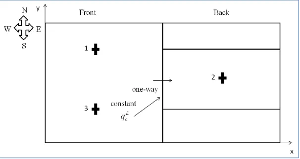
In our application of interest of wind-farm design, we need to move turbines to identify the optimal layout – one that maximizes power production. To attain this objective we create a ‘tile’ for each turbine or a group of turbines and define an associated basis. The tiles can then be assembled at run-time for fast investigation of power production. The assembling currently was limited to movements in a single direction (Y/transverse) [3] as Figure 1, left side depicts. In this report we will study movement of tiles in the 2D plane.
Figure 1: Tile movement Left: Y/Transverse direction; Right: X/Longitudinal direction. The crosses depict turbine positions.
Notwithstanding the rule of thumb for distance between wind-turbines, that wind-farm designers often use, it is useful a tool for designers to have the capability to move the turbines in a plane and get estimates of flow fields in addition to the power production. The planar movement of tiles is also a good starting point to study the feasibility of the method for complex terrain. Complex terrain adds more degrees to the solution.
By studying the effect of number of basis and snapshots on the fidelity of the solution for a planar tile movement we will be able to make initial estimates of the ‘amount of information’ needed in performing model reduction on complex terrain. While the focus is currently on predicting the power production, the model reduction technique could also be used in predicting the loads and stresses on the turbine. We estimate L2 norm of the difference between CFD and the model reduction for the 3 components of velocity.
The report is prepared as follows. The generation of the basis B is described in the next section 2.2. The methods for computing coefficients, are described in section 2.3. The results are presented in section 0 followed by the summary of what we have learnt in section 2.5.
2.2 Generating Basis (B)
The basis is generated from the ‘snapshots’ of the ‘off-line’ CFD solutions. The CFD solutions generated use an actuator-disk model to represent the influence of the turbines. The snapshots are of different situations that we expect to arise. The basis and hence the reduced solution is thus going to be able to, at best, represent the situations in the CFD solutions.
These snapshots collected together, C, are then subjected to an ‘economical’ Singular Value Decomposition (SVD) to obtain the desired orthonormal set of basis vectors (the left and right singular vectors B and V respectively):
(2)
Let P be the number of snapshots and N the size of the domain simulation. Then C is , B is , S is and V is in eq (2).
The left singular vectors, B, have the property that they span the same space (range) as the collection of snapshots, C. Also the vectors in B are arranged in a descending order based on the singular values (diagonal values in S). We can now construct a reduced space by picking the first columns in B, where M<<N.
Both the actuator-disk model and the SVD have been implemented in OpenFoam.
2.3 Computing Coefficients (a)
The key to using model reduction is in the methodology used in computing the weights a. As mentioned earlier we’ll be using the tiles to describe the flow-fields around turbines.
We are going to use two kinds of constraints to obtain the coefficients:
1) Minimize discrepancy between tiles at the tile boundary interface we, i.e., the boundary-matching condition.
2) Ensure that the solution is ‘physically meaningful’, i.e., it satisfies the Reynolds Averaged Navier-Stokes (RANS) Equations, as well as possible –RANS condition.
For now, following Heggelund et al[3], we’ll be ignoring the fact that across tile boundaries mass conservation/continuity constraint will not be satisfied. This is because our main concern is production estimates for the turbines and not finer details of the flow-field. However it may be possible, on the lines of SIMPLE scheme in CFD, to include the continuity constraints in the RANS equations and get a more physically meaningful reduced solution. This is something we have not studied and should be investigated later.
Let the state vector q, basis B and coefficient a for tile i be defined as: [ ] [ ] [ ] (3) The elements making up the state vector q are the three components of velocity (u, v, w), total viscosity (
, sum of molecular and eddy viscosity), pressure (p) and turbulent kinetic energy (k).For either one or/and both the constraints we’ll define an associated objective function, F(a), based on a, that we will minimize. We then estimate production from each turbine when we move the back turbine in the x and y direction and the x-y plane.
2.4 Inflow Boundary Condition – One way coupling
We start with the simpler situation where the front tile in Figure 2 is kept constant.Figure 2: Two-tile configuration with 1-way coupling. Crosses depict turbine positions. Front tile includes turbines 1 and 3.
We would thus like to minimize the function:
‖ ‖ (4)
where the superscripts represent projection in a given direction (W for West etc.) and the subscript c stands for ‘constant’.
Clearly, such a function is minimized when:
(5)
where ( ) and ( ) (6)
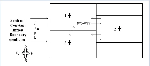
2.5 Inflow Boundary Condition – Two - way coupling
The next level of complexity is when we include one tile for each turbine and do a two-way coupling where coefficients ai need to be defined for each tile.Here the constraint will be the more realistic inflow-boundary condition which is treated as a constant, see Figure 3:
Figure 3: Three-tile configuration with 2-way coupling. Crosses depict turbine positions.
The objective function now becomes:
[ ‖ ‖ ‖ ‖ ‖ ‖ ‖ ‖ ‖ ‖ ] (7a)
which can be generalised to:
‖ ̃ ̃ ‖ (7b)
In minimizing the above function like in Eq. 5 (one-way coupling), expression for A and b are:
̃ ̃ = [ ( ) ( ) ( ) ( ) ( ) ( ) ( ) ( ) ( ) ( ) ( ) ( ) ( ) ( ) ( ) ( ) ( ) ( )] ̃ ̃ [ ] (8)
2.5.1 RANS Equations
Here we bring into consideration that the fluid flow-field that we are solving for should be as close as possible in satisfying the governing equations, i.e., RANS equations (we will keep our focus on the steady state version).
The steady state, incompressible RANS equations, with body forces ignored, is given by:
(9)
where the molecular and eddy/turbulent viscosity combined together are given by:
(
)
(10)
The RANS equations upon discretisation can be defined by operators acting on the state variable q. We follow Heggelund et al and define them as: advection, pressure, viscosity and turbulent kinetic energy operators. Each term is discretised using the 2nd order central differencing scheme (Appendix A). The discretised equation in operator form is as follows:
( ) (11)
The subscript q, in the equation represents the dependence of the operators on the state variable q. Representing q in its basis representation and pre-multiplying Eq. (12) BT we get:
( ) (12)
The viscosity and the advection terms, Aq and Vq together can thus be third
order tensors while P and K will be 2nd order tensors. The issues we ran into with the operators are described in Appendix A. We can thus represent the RANS equation in its ‘exact form’ as:
0
ij j j k ijkx
x
L
x
T
(13)and the objective function for the RANS equation as:
j ij j k ijk i
T
x
x
L
x
x
F
(
)
(14)2.5.2 Combined Objective Function
The combined objective function for both the boundary matching and RANS equations can be written as:
where
is a scalar between 0 and 1; it represents the compromise between boundary matching condition and the RANS2 conditionThis objective function (non-linear 4th- order) is solved using the Newton-Raphson method. We use the analytical expressions for the gradient and hessian of the objective function in the optimization algorithm.
{ ̃ ̃ ̃ } (16) { ̃ ̃ ( ) ( )( ) } (17)
Heggelund et al [3] uses a common basis for all tiles which seems reasonable when RANS equations provide larger contribution to the objective function. While using a common basis is convenient and efficient when generalizing the application, it must be borne in mind that the flow-physics of the two front-tiles and the back tile are different. Thus, in the studies performed below we used two sets of basis; one for the two front tiles and a second basis for the back tiles.
The parameter represents a tradeoff between matching the tile boundaries versus the momentum equations. If the model is used for production estimates, higher values should be used. If visual appearance is important (i.e. continuity across tiles) a lower values should be used. The best choice of parameters also depends on the number of tiles.
Without enforcing the RANS equations (i.e 0) in the optimization we were able to obtain the best results i.e. using only the boundary matching as optimisation criteria.
We have noticed that a large number of basis vectors may introduce unphysical modes of behaviour, and emphasizing RANS equations can suppress such undesirable modes of behaviour.
So far, better results were achieved by omitting the RANS equations in the objective function (i.e. the second term in Eq. (15)). Comparing our implementation to the work of Heggelund et al [3], our error terms are typically higher for the second term of the Eq. (15). The difference in implementation is the choice of discretisation scheme of the viscosity term in Eq. (11), see Appendix A for further explanation. A modification of the discretisation scheme is believed to provide a more precise representation of the viscosity terms and thus lower error terms, and is now being updated on the website.
It would make an interesting study to compare the two methodologies of using different set of basis vectors, keeping the total bytes of information as constant, but we will not be pursuing it at this point.
A brief discussion on which criteria to use in the objective function for optimising the coefficients for the basis vectors is provided in section 4.1.
3 Results
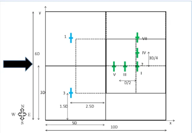
Two sets of simulations with different setups were run, one each in OpenFoam and WindSim. Both the methods used the Actuator Disk model to simulate the effects of the turbine, see Figure 4 and Figure 5.
Figure 4 OpenFoam simulation setup. The model contain three turbines contained in tiles 1,2,3. The back tile is moved in various positions creating snapshots that generate various flow patterns. The back tile is moved traverse in seven snapshots from the central position, here illustrated by snapshot I, IV and VII. The back tiles is then moved in longitudinal direction through five snapshots (marked I to V and illustrated by I, III and V). In total, 11 snapshots were generated from the OpenFoam CFD model.
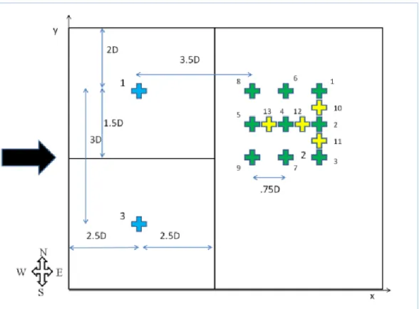
Figure 5: WindSim simulation setup. Similar to the OpenFoam setup, the simulation model contains three turbines contained in tiles 1,2,3. The back tile (tile 2) is moved intovarious positions to create various flow patterns for the snapshots. The back tile turbine position is numbered from 1..13, creating a total of 13 snapshots.
The first set of simulations in OpenFoam were performed to:
i)
Verify and validate the software capability in transverse tile movement,
ii)
Verify the capability of tile movement in longitudinal direction and,
iii)
Study ‘elastic limit’, or how little information can we use, of the model
reduction technique using tiles for planar tile movement with reasonable
agreement of the solution.
For verification and validation boundary matching error, production estimate error and error in the prediction of the velocity components for the tile 2 were performed.
We next look at the error in production and velocity predicted from Model Reduction by a direct comparison with results from the CFD. The error in production is computed as a relative error, that is,
100
%
Prod
Prod
Prod
=
Error
Production
Relative
CFD CFD MR
(18)and the error in velocity is computed as an L2 norm:
2
CFD
MR
U
U
(19) It must be mentioned at this point that the L2 norm is not normalized by the total number of grid points but is given as a representative of total error in the back tile.The second set of simulations in WindSim is what is likely to be used in the planar tile movement and we intend to use it to study the accuracy of the model reduction technique when compared with CFD. The study provides a contrast on the type of set-up ideal for model reduction for a planar tile movement as well as focuses on the amount of information necessary in getting reasonable results with Model Reduction.
3.1 OpenFoam Simulations
The OpenFoam simulations were as follows:
Transverse Tile Movement - 7 CFD snapshots/simulations for the tile 2
movement in Y/transverse direction.
Longitudinal Tile Movement - 5 CFD cases were run for the tile 2 movement in
X/longitudinal direction.
One of the simulations was common to both, providing 11 independent CFD simulations.
Each simulation has a grid size of 120x72x72.
The size of tile size is 60x36x72
The rotor diameter D is 36m.
The physical extent of the domain is 10D (360m) in x and 6D (216m) in y and z.
3.1.1 Transverse tile movement
Boundary matching error was compared using
a) basis computed from 7 snapshots in the transverse direction, b) basis from all 11 snapshots.
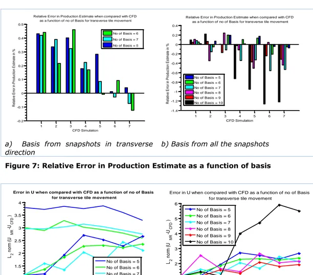
It is seen that with number of basis > 5, the boundary matching error from b) is lesser than a). This is encouraging and important since in planar tile movement we will be using all the snapshots. Boundary matching errors and L2 norms for each velocity component is presented in Figure 6 through Figure 10:
a) Solid line: Basis from snapshots in trans-verse direction. Dotted line: Basis from all the snapshots
b) Dotted line: basis from all the snapshots.
Figure 6: Boundary Matching Error as a function of basis.
a) Basis from snapshots in transverse direction
b) Basis from all the snapshots
Figure 7: Relative Error in Production Estimate as a function of basis 110 120 130 140 150 160 0 1 2 3 4 5 y-Location (m) B o u n d a ry M a tc h in g E rr o r
Boundary Matching Error as a function of basis for transverse tile movement
No of Basis = 5 No of Basis = 6 No of Basis = 7 100 110 120 130 140 150 160 0 2 4 6 8 10 12 y-Location (m) B o u n d a ry M a tc h in g E rr o r
Boundary Matching Error as a function of basis for transverse tile movement # basis= 5 # basis= 6 # basis= 7 # basis = 8 # basis = 9 # basis= 10 1 2 3 4 5 6 7 -0.2 -0.1 0 0.1 0.2 0.3 0.4 0.5 CFD Simulation R e la tiv e E rr o r in P ro d u ct io n E st im a te in %
Relative Error in Production Estimate when compared with CFD as a function of no of Basis for transverse tile movement
No of Basis = 6 No of Basis = 7 No of Basis = 5 1 2 3 4 5 6 7 -1.4 -1.2 -1 -0.8 -0.6 -0.4 -0.2 0 0.2 0.4 CFD Simulation R e la tiv e E rr o r in P ro d u ct io n E st im a te in %
Relative Error in Production Esitmate when compared with CFD as a function of no of Basis for transverse tile movement
No of Basis = 5 No of Basis = 6 No of Basis = 7 No of Basis = 8 No of Basis = 9 No of Basis = 10 1 2 3 4 5 6 7 1 1.5 2 2.5 3 3.5 4 CFD Simulation L2 n o rm ( U MR -U C F D )
Error in U when compared with CFD as a function of no of Basis for transverse tile movement
No of Basis = 5 No of Basis = 6 No of Basis = 7 1 2 3 4 5 6 7 1 2 3 4 5 6 CFD Simulation L2 n o rm ( U MR -U C F D )
Error in U when compared with CFD as a function of no of Basis for transverse tile movement
No of Basis = 5 No of Basis = 6 No of Basis = 7 No of Basis = 8 No of Basis = 9 No of Basis = 10
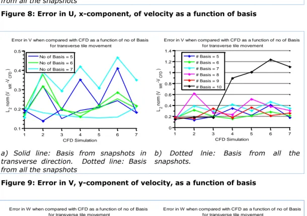
a) Solid line: Basis from snapshots in transverse direction. Dotted line: Basis from all the snapshots
b) Dotted line: Basis from all the snapshots.
Figure 8: Error in U, x-component, of velocity as a function of basis
a) Solid line: Basis from snapshots in transverse direction. Dotted line: Basis from all the snapshots
b) Dotted lnie: Basis from all the snapshots.
Figure 9: Error in V, y-component of velocity, as a function of basis
a) Solid line: Basis from snapshots in transverse direction. Dotted line: Basis from all the snapshots
b) Dotted line: basis from all the snapshots.
Figure 10: Error in W, z-component of velocity, as a function of basis
The error in production decreases with number of basis in general but suddenly shoots up for 10 basis vectors as tile 2 is moved towards tile 1 (Figure 14). Even with 10 bases the error is quite small (~1% in production and ~6 for U and ~1.2 for V and W). We know that the wake-interaction between turbines increases as we move tile 2 towards tile 1. Thus there’s more change in the flow as we move the tile 2. The boundary matching term only ensures that the discrepancy in values across the tile boundaries are small (Figure 6). It does not necessarily ensure that the flow change has been accurately addressed. 1 2 3 4 5 6 7 0.1 0.2 0.3 0.4 0.5 CFD Simulation L2 n o rm ( V MR -V C F D )
Error in V when compared with CFD as a function of no of Basis for transverse tile movement
No of Basis = 5 No of Basis = 6 No of Basis = 7 1 2 3 4 5 6 7 0 0.2 0.4 0.6 0.8 1 1.2 1.4 CFD Simulation L2 n o rm ( V MR -V C F D )
Error in V when compared with CFD as a function of no of Basis for transverse tile movement
# Basis = 5 # Basis = 6 # Basis = 7 # Basis = 8 # Basis = 9 # Basis = 10 1 2 3 4 5 6 7 0 0.1 0.2 0.3 0.4 0.5 CFD Simulation L2 n o rm ( W MR -W C F D )
Error in W when compared with CFD as a function of no of Basis for transverse tile movement
No of Basis = 5 No of Basis = 6 No of Basis = 7 1 2 3 4 5 6 7 0 0.2 0.4 0.6 0.8 1 1.2 1.4 CFD Simulation L2 n o rm ( W MR -W C F D )
Error in W when compared with CFD as a function of no of Basis for transverse tile movement
# Basis= 5 # Basis= 6 # Basis= 7 # Basis = 8 # Basis= 9 # Basis= 10
The flow field of the reduced model is presented in Figure 11 for 7 and 10 basis vectors respectively. The reconstruction of the flow field provides significant reduction in dimensionality.
a) Contour plot for U with 7 basis vectors.
Figure 11: Effect of number of basis on boundary matching and physical variables (U)
The higher basis can be considered equivalent to the high frequency components of a Fourier series. In a Fourier series by adding high frequency components we risk increasing dispersion error and not necessarily representing the curve better. The high frequency components can be ‘noisy’ and have the capability of distorting the physics. It is for this purpose the RANS operators and optimization will be useful and effective. The SVD algorithm may also play a role here but has not been investigated.
3.1.2 Longitudinal tile movement
Results from longitudinal movement of the reduced model of the OpenFoam CFD simulations are presented below. 5 CFD cases were run for the tile 2 movement in X/longitudinal direction.
The boundary matching error was compared using
a) Basis computed from 5 snapshots in the longitudinal direction, b) Basis from all 11 snapshots.
It is seen that with more than three basis, boundary matching errors from b) is comparable to a). Also with increase in basis computed from all the snapshots the boundary matching term further reduces, as can be seen in Figure 12.
a) Solid line: Basis from snapshots in longitudinal direction. Dotted line: Basis from all the snapshots
b) Solid line: Basis from all the snapshots
Figure 12: Boundary matching as a function of number of basis for longitudinal movements.
a) Basis from snapshots in longitudinal
direction. b) Basis from all the snapshots.
Figure 13: Relative Error in Production Estimate as a function of basis for longitudinal movements. 230 240 250 260 270 0 2 4 6 8 10 x-Location (m) B o u n d a ry M a tc h in g E rr o r
Boundary Matching Error as a function of basis for Longitudinal tile movement
# Basis = 3 # Basis = 4 # Basis = 5 230 240 250 260 270 0 0.5 1 1.5 2 x-Location (m) B o u n d a ry M a tc h in g E rr o r
Boundary Matching Error as a function of basis for Longitudinal tile movement
No of Basis = 5 No of Basis = 6 No of Basis = 7 No of Basis = 8 No of Basis = 9 No of Basis = 10 0 1 2 3 4 5 6 -0.1 0 0.1 0.2 0.3 0.4 0.5 0.6 CFD Simulation R e la tiv e E rr o r in P ro d u ct io n E st im a te in %
Relative Error in Production Esitmate when compared with CFD as a function of no of Basis for Longitudinal tile movement
No of Basis = 3 No of Basis = 4 No of Basis = 5 0 1 2 3 4 5 6 -0.3 -0.2 -0.1 0 0.1 0.2 0.3 0.4 0.5 0.6 CFD Simulation R e la tiv e E rr o r in P ro d u ct io n E st im a te in %
Relative Error in Production Esitmate when compared with CFD as a function of no of Basis for Longitudinal tile movement
# Basis=5 # Basis=7 # Basis=8 # Basis=9 # Basis=10 # Basis=6
a) Solid line: Basis from snapshots in longitudinal direction. Dotted line: Basis from all the snapshots
b) Solid line: Basis from all the snapshots.
Figure 14: Error in U, x-component, of velocity as a function of basis
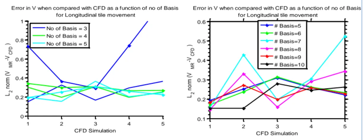
a) Solid line: Basis from snapshots in longitudinal direction. Dotted line: Basis from all the snapshots
b) Solid line: Basis from all the snapshots.
Figure 15: Error in V, y-component, of velocity as a function of basis
1 2 3 4 5 0 1 2 3 4 5 6 7 CFD Simulation L2 n o rm ( U MR -U C F D )
Error in U when compared with CFD as a function of no of Basis for Longitudinal tile movement
No of Basis = 3 No of Basis = 4 No of Basis = 5 1 2 3 4 5 1 1.5 2 2.5 3 3.5 CFD Simulation L2 n o rm ( U MR -U C F D )
Error in U when compared with CFD as a function of no of Basis for Longitudinal tile movement
# Basis=5 # Basis=6 # Basis=7 # Basis=8 # Basis=9 # Basis=10 1 2 3 4 5 0 0.2 0.4 0.6 0.8 1 CFD Simulation L2 n o rm ( V MR -V C F D )
Error in V when compared with CFD as a function of no of Basis for Longitudinal tile movement
No of Basis = 3 No of Basis = 4 No of Basis = 5 1 2 3 4 5 0.1 0.2 0.3 0.4 0.5 0.6 CFD Simulation L2 n o rm ( V MR -V C F D )
Error in V when compared with CFD as a function of no of Basis for Longitudinal tile movement
# Basis=5 # Basis=6 # Basis=7 # Basis=8 # Basis=9 # Basis=10 1 2 3 4 5 0.2 0.4 0.6 0.8 1 1.2 1.4 1.6 CFD Simulation L2 n o rm ( W MR -W C F D )
Error in W when compared with CFD as a function of no of Basis for Longitudinal tile movement
No of Basis = 3 No of Basis = 4 No of Basis = 5 1 2 3 4 5 0.1 0.2 0.3 0.4 0.5 0.6 0.7 0.8 CFD Simulation L2 n o rm ( W MR -W C F D )
Error in W when compared with CFD as a function of no of Basis for Longitudinal tile movement
# Basis=5 # Basis=6 # Basis=7 # Basis=8 # Basis=9 # Basis=10
a) Solid line: Basis from snapshots in longitudinal direction. Dotted line: Basis from all the snapshots
b) Solid line: Basis from all the snapshots
Figure 16: Error in W, z-component, of velocity as a function of basis
Production errors reduce with increasing number of basis in general and unlike the transverse tile movement it does not suddenly shoot up as the tile 2 is moved towards tile 1 and 3 (compare Figure 13 - Figure 16 with Figure 7-Figure 10). Also the error in velocities is quite small and in general decreases with basis size. In general the physics of the flow-field does not change drastically when we move the turbine 2 in the longitudinal direction. Also the production increases as we move the turbine 2 closer to 1 and 3. Hence for longitudinal tile movement RANS operators and optimization can probably be avoided.
3.1.3 Planar Tile Movement
Planar tile movement is the important capability that we are testing and studying in this project. As mentioned earlier this study will also have a bearing on the prospects of using the current methodology, of using tiles, in performing model reduction for complex terrain.
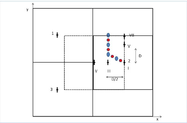
We are studying the setup as shown in Figure 17. We use all the 11 original snapshots for computing the basis. The reduced solution is computed along a trajectory shown by the red dots. The blue dots are where we perform CFD simulations and compare it with the reduced solution at the same position in addition to the location I.
Figure 17: Setup for planar tile study. The red dots depict the positions for generating snapshots for the reduced model, leading to a trajectory in moving in both transverse and longitudinal direction. The blue dots shows the
positions where we compare the original CFD model with the reduced model. We look at the same parameters as studied in longitudinal and transverse tile movement, see Figure 18 - Figure 19.
a) Basis 3-5 from all the snapshots b) Basis 6-10 from all the snapshots
Figure 18: Boundary Matching Error as a function of basis.
Consistent with earlier observation boundary matching error reduces with increase in number of basis (see Figure 18). The boundary matching error is, as expected, larger in magnitude when compared to longitudinal and transverse tile movement.
Figure 19: Relative Error in Production Estimate as a function of basis 100 120 140 160 180 0 100 200 300 400 y-Location (m) B o u n d a ry M a tc h in g E rr o r
Boundary Matching Error as a function of basis for Planar tile movement
No of Basis = 3 No of Basis = 4 No of Basis = 5 100 110 120 130 140 150 160 170 0 20 40 60 80 100 120 140 160 y-Location (m) B o u n d a ry M a tc h in g E rr o r
Boundary Matching Error as a function of basis for Planar tile movement
# Basis=5 # Basis=6 # Basis=7 # Basis=8 # Basis=9 # Basis=10 1 2 3 4 5 -2 -1.5 -1 -0.5 0 0.5 1 1.5 2 CFD Simulation R e la tiv e E rr o r in P ro d u ct io n E st im a te in %
Relative Error in Production Esitmate when compared with CFD as a function of no of Basis for Planar tile movement
No of Basis = 5 No of Basis = 6 No of Basis = 7 No of Basis = 8 No of Basis = 9 No of Basis = 10
The error increases as we move further out closer to tile 1, which was also expected. However the error shows approximately a linear growth beyond location 6. Location 6 happens to be the point beyond which we move only in the y-direction. Significantly enough, the relative error in production is within ~1.5% (Figure 19). That’s encouraging if production estimation is our sole objective. However we’d like to know the limitation in prediction of the flow variables, see Figure 20 to Figure 22.
a) Basis 3-5 from all the snapshots b) Basis 5-10 basis from all the snapshots
Figure 20: Error in U, x-component, of velocity as a function of basis
a) Basis 3-5 from all the snapshots b) Basis 5-10 from all the snapshots
Figure 21: Error in V, y-component, of velocity as a function of basis
1 2 3 4 5 0 5 10 15 20 25 30 35 40 CFD Simulation L2 n o rm ( U MR -U C F D )
Error in U when compared with CFD as a function of no of Basis for Planar tile movement
No of Basis = 3 No of Basis = 4 No of Basis = 5 1 2 3 4 5 0 5 10 15 20 CFD Simulation L2 n o rm ( U MR -U C F D )
Error in U when compared with CFD as a function of no of Basis for Planar tile movement
No of Basis = 5 No of Basis = 6 No of Basis = 7 No of Basis = 8 No of Basis = 9 No of Basis = 10 1 2 3 4 5 0 0.5 1 1.5 2 CFD Simulation L2 n o rm ( V MR -V C F D )
Error in V when compared with CFD as a function of no of Basis for Planar tile movement
No of Basis = 3 No of Basis = 4 No of Basis = 5 1 2 3 4 5 0 0.5 1 1.5 2 2.5 3 CFD Simulation L2 n o rm ( V MR -V C F D )
Error in V when compared with CFD as a function of no of Basis for Planar tile movement
No of Basis = 5 No of Basis = 6 No of Basis = 7 No of Basis = 8 No of Basis = 9 No of Basis = 10
a) Basis 3-5 from al the snapshots b) Basis 5-10 from all the snapshots
Figure 22: Error in W, z-component, of velocity as a function of basis
Figure 20 to Figure 22 shows that error in velocity prediction for number of basis >7 is of comparable magnitude to the transverse tile movement and of the same order as the longitudinal tile movement. Expectantly the error in U is greater because of the larger fluctuations across turbines. The error in V and W is smaller because of the smaller change they undergo.
All in all the method looks promising and we proceed to the WindSim simulation which we expect to be the more ‘canonical’ situation to be used in practice. 1 2 3 4 5 0 0.5 1 1.5 2 CFD Simulation L2 n o rm ( W MR -W C F D )
Error in W when compared with CFD as a function of no of Basis for Planar tile movement
No of Basis = 3 No of Basis = 4 No of Basis = 5 1 2 3 4 5 0 0.5 1 1.5 2 2.5 CFD Simulation L2 n o rm ( W MR -W C F D )
Error in W when compared with CFD as a function of no of Basis for Planar tile movement
# Basis=5 # Basis=6 # Basis=7 # Basis=8 # Basis=9 # Basis=10
3.2 WindSim Simulations
In total 13 WindSim simulations were run with different positions for the back turbine tile 2 as shown in Figure 23. The diameter, D, of the turbine used was 90m. The figures follow the same numbering for comparison with CFD simulations. The WindSim simulations were performed using a non-uniform grid, and the CFD results were then interpolated (3D) onto a regular grid (180x128x32) to fit the format for our model reduction program.
Figure 23: Setup of tiles when extracted from 13 WindSim CFD results. The green and yellow crosses represent the various turbine postions for which snapshots were generated.
We performed two tests to see how different selections of snapshots for the basis influence the model reduction accuracy.
3.2.1 WindSim snapshot set I
In this case study we use the snapshots obtained from simulations in green from Figure 23 as basis for the model reduction. The reduced solution is computed at the yellow locations, to calculate the accuracy in production estimates and velocity components for a varying number of basis vectors.
Figure 24: Relative Error in Production Estimate as a function of basis
a) U, v-component of velocity
b) V, y-component of velocity. c) W, z-component of velocity
Figure 25: U,V,W - components of velocity.
1 2 3 4 5 6 7 8 9 10 11 12 13 -30 -20 -10 0 10 20 30 CFD Simulation R e la tiv e E rr o r in P ro d u ct io n E st im a te in %
Relative Error in Production Esitmate when compared with CFD as a function of No of Basis for Planar tile movement
# Basis = 5 # Basis = 6 # Basis = 7 # Basis = 8 # Basis = 9 0 2 4 6 8 10 12 14 0 50 100 150 200 250 CFD Simulation L2 n o rm ( U MR -U C F D )
Error in U when compared with CFD as a function of No of Basis for Planar tile movement
No of Basis = 5 No of Basis = 6 No of Basis = 7 No of Basis = 8 No of Basis = 9 0 2 4 6 8 10 12 14 0 5 10 15 20 25 30 35 CFD Simulation L2 n o rm ( V MR -V C F D )
Error in V when compared with CFD as a function of No of Basis for Planar tile movement
No of Basis = 5 No of Basis = 6 No of Basis = 7 No of Basis = 8 No of Basis = 9 0 2 4 6 8 10 12 14 0 5 10 15 20 25 30 35 CFD Simulation L2 n o rm ( W MR -W C F D )
Error in W when compared with CFD as a function of No of Basis for Planar tile movement
No of Basis = 5 No of Basis = 6 No of Basis = 7 No of Basis = 8 No of Basis = 9
Figure 24 and Figure 25 shows that the results using WindSim for snapshots are poor compared to the results obtained when using OpenFOAM snapshots. This is clearly seen when the results are compared a bit more in details. CFD simulation for snapshot 2, 12, 4, 13 (i.e. longitudinal movement) from WindSim are plotted in Figure 26.
Figure 26: CFD simulations from WindSim. CFD simulation for snapshot 2 (upper left ), 12 (upper right), 4 (lower left) and 13 (lower right)
Likewise, the longitudinal CFD simulations are presented in Figure 27 as snapshots 1,2,3,4 from OpenFoam.
Figure 27 Longitudinal CFD simulations from OpenFoam. Longitudinal CFD simulations 1 (upper left), 2 (upper right), 3 (lower left) and 4 (lower right) for from OpenFoam
The results cannot be compared directly, because different boundary conditions, actuator disk properties, discretization schemes, etc. has been used.
We look at the singular values for the tile 2 based on the WindSim snapshot set I and compare it with the singular values from OpenFoam, see Figure 28 and Figure 29.
a) Snapshot set I b) All snapshots
Figure 28: Singular Values from WindSim simulation
a) Longitudinal snapshots b) All snapshots
Figure 29: Singular Values from OpenFoam simulation
There’s a substantial separation between the singular values (and consequently the basis vectors) in OpenFoam even with 5 snapshots. In WindSim the drop in singular values is not substantial. This means that there’s not enough ‘distance’ or distinction between the basis vectors especially between 3 to 8 basis vectors.
As was mentioned in the beginning, we proceed to the WindSim snapshot set II with not much optimism in getting improved results.
3.2.2 WindSim snapshot set II
This set of snapshots is outlined as green crosses in Figure 30. These snapshots are used then to compute the reduced solutions at the yellow locations in order to assess the errors in production estimates and velocity components. 0 2 4 6 8 10 101 102 103 104 105
Singular Value/Basis Vector for tile2
Sin gu lar Va lue s
Singular Values of tile 2 for WindSim
0 5 10 15 101 102 103 104 105
Singular Value/Basis Vector for tile 2
S in g u la r V a lu e s
Figure 30: Snapshot set II for WindSim. Yellow locations used as snapshots for lateral movement of turbines.
Figure 31: Relative Error in Production Estimate as a function of basis
1 2 3 4 5 6 7 8 9 10 11 12 13 -20 0 20 40 60 80 CFD Simulation R e la tiv e E rr o r in P ro d u ct io n E st im a te in %
Relative Error in Production Esitmate when compared with CFD as a function of No of Basis for Planar tile movement
No of Basis = 5 No of Basis = 6 No of Basis = 7 No of Basis = 8 No of Basis = 9
a) Error in U - velocity component as
function of basis
b) Error in V - velocity component as
function of number of basis c) Error in W - velocity component as function of number of basis Figure 32: Error in U,V,W - velocity component as a function of basis Figure 31 and Figure 32 shows that results for snapshot set II are similar to the ones obtained with the snapshot set I. Like in snapshot set I we also look at the singular values for snapshot set II (see Figure 33) and come to the same conclusions as before.
0 5 10 15 0 50 100 150 200 250 300 CFD Simulation L2 n o rm ( U MR -U C F D )
Error in U when compared with CFD as a function of No of Basis for Planar tile movement
No of Basis = 5 No of Basis = 6 No of Basis = 7 No of Basis = 8 No of Basis = 9 0 5 10 15 0 5 10 15 20 25 30 CFD Simulation L2 n o rm ( V MR -V C F D )
Error in V when compared with CFD as a function of No of Basis for Planar tile movement
No of Basis = 5 No of Basis = 6 No of Basis = 7 No of Basis = 8 No of Basis = 9 0 5 10 15 0 5 10 15 20 25 30 CFD Simulation L2 n o rm ( W MR -W C F D )
Error in W when compared with CFD as a function of No of Basis for Planar tile movement
No of Basis = 5 No of Basis = 6 No of Basis = 7 No of Basis = 8 No of Basis = 9
a) Snapshot set II b) Longitudinal Snapshots from OpenFoam Figure 33 Singular value comparison between openFoam and WindSim
The reason for the results obtained using the WindSim results has not been identified. Some possible explanations are:
- As the velocity deficit is larger behind the turbines in the WindSim simulations (higher CT), the boundary matching is performed in a region of high transverse gradients. This might call for higher order discretization schemes.
- WindSim use non-equilibrium inlet profiles for the turbulent kinetic energy, causing slight changes in the profile for turbulent kinetic energy and velocity when simulating flow over a flat terrain. This causes the rear turbine to operate under slightly different conditions depending on the stream-wise position. This effect causes a difference in the free-stream velocity of approximately 0.2% between position 1 and 8. This is small but might be enough to add noise to the results.
3.3 Summary of results
Two-way tile coupling with separate basis has been successfully implemented, and studied on two sets of flow-fields generated in OpenFoam and WindSim, both using actuator-disk model. Model reduction performed on the OpenFoam flow shows promising results in longitudinal, transverse and planar tile movement even without incorporating Newton-Raphson optimization through RANS equations.
More systematic and canonical studies were to be performed from the WindSim CFD solutions. The reason for this has not been identified, but two possible explanations are presented:
- The higher C
T-value used in the WindSim simulations give higher
transverse gradients, demanding a higher order discretization
scheme
- Non-equilibrium inlet profiles for turbulent kinetic energy used in
WindSim causes differences in free stream flow parameters in
different solutions, adding noise to the results.
4 Discussion and conclusion
A reduced model of a steady RANS CFD actuator-disc model of a three turbine configuration was successfully implemented. The model consists of turbine tiles that can be moved independently in the plane, where each turbine tile is represented by a linear combination of the basis vectors in reduced space. Since the order of the reduced model is much smaller than the full RANS model, the flow field can be computed much faster. Updating the tile flow field requires minimization of
2 2 2 2~
~
1
2
1
)
(
x
iA
ijx
jb
iT
ijkx
kx
jL
ijx
jF
(20)which is computed in less than a second for the reduced model. In our case the RANS model is of order N = 120x72x72 and the reduced model is of order M = 3x7 – a reduction by a factor of 104
4.1 Planar movement of tiles
Previous studies analyzed transversal movement of tiles [3]. Our finding is that errors in the velocity components are low for transversal movement of tiles and errors in production estimates is approximately 1%3.
We have extended the model to longitudinal movement of turbines and find that the errors are of the same magnitude as transversal movement. In fact errors reduce systematically with increasing number of basis vectors. The physics change less in longitudinal direction and it seems boundary matching is less important than for transversal movement.
Planar movement (both transversal and longitudinal) increase errors compared to transversal and longitudinal movement, but are still considered low. The production estimate errors are approximately 1.5%, which is acceptable compared to the uncertainty of underlying CFD models from which the basis solutions are extracted4.
Our tests show that model reduction can be achieved with low errors for a limited number of basis vectors. The required number of basis vectors increase in the case of planar movement.
In our test cases, boundary matching has been sufficient to enforce physical behavior of the reduced model. While errors reduce with increasing number of basis, we observed a sudden jump in errors in the case of transversal movement unless we enforce the RANS momentum equations. Unphysical modes of behavior may occur when introducing too many basis modes. The second term in Eq. (20) seeks to avoid such modes of behavior.
3 See eq. (18) in chapter 3
A continuity operator can be included in the same way as the RANS operators, see Eqs. (11) and (12). In future work, the most effective combination of boundary matching, matching the RANS equations and/or continuity equations should be investigated further.
About 65% of the basis vectors in our case studies were needed, which suggests there is a potential for applying model reduction to more complex CFD models.
4.2 Uncertainty of CFD models and the reduced model
Insights from two wake model blind test competitions show that RANS actuator disk models perform comparatively well in situations of multiple wakes and high turbulence. Agder Energi and CMR participated in a blind test study involving a range of different CFD models from standard Blade Element Momentum (BEM) methods to advanced fully resolved Computational Fluid Dynamics (CFD) models. The results varied (+/-) 10% in predicting power generation and thrust force, while there is a much larger uncertainty in predicting the wake turbulence field [7]. The study states that it was not possible to conclude that the fully resolved CFD models predictions were superior to the simpler BEM models.In a follow-up of the first blind test, a downstream turbine was introduced to the experiment [8]. While simulations results were comparable to the first blind test, RANS models improve their performance as the turbulence becomes more isotropic. Such conditions can be expected in complex terrain. At sea, ambient turbulence is lower, and the wake structure breaks down more slowly.
The models included in the blind test are not commonly used by the industry. CFD models are used for flow field calculations of the farm, while the simpler models of Jensen [9] and Frandsen [10] are used to represent wake deficit and wake turbulence calculations. Only a few full studies exist where entire wind farms are simulated using actuator disk methods.
The minimum total uncertainty in production estimates in current state-of-the-art wind resource assessment is considered to be 10% based on Meventus’ experience. A survey under the EU WAUDIT programme holds similar estimates on uncertainty [11].
The errors introduced by model reduction are therefore acceptable compared to the degree of uncertainty in the numerical CFD models themselves. We have only analyzed the errors of one downstream turbine involving three tiles. With cascading tiles downstream, errors may propagate. This is left for future work.
We have shown that the method of model reduction can be used to represent wind flow simulations with a major reduction in dimensionality (~104) and at a minor increase in errors (~1.5%). This allows reduced models to be recalculated within seconds, suitable for interactive visualisation and
optimisation purposes. The precision can be controlled by the number of snapshots and the corresponding selection of basis vectors.
4.3 Future work
Extending the model to full planar movement
Although we have demonstrated model reduction of planar movement of turbines, the movement is restricted to the region of overlapping tiles. Introducing empty tiles with a separate basis could be a way to allow free movement of turbines in a reduced model. Another approach could be to introduce turbine tiles with different length.
Errors of cascading wakes
The error propagation of cascading wakes must be also be addressed by increasing the model size.
The above issues will be addressed by applying the model reduction technique on the Sheringham Shoal offshore plant.
Extension to complex terrain
Until now we have only considered flat terrain, and the interaction of turbine wakes. When introducing complex terrain, the local flow fields around turbines do not only depend on the location of other turbines, but on the location of the turbine itself due to terrain features. The wind flow over terrain is also directional dependent and an increased number of basis vectors most likely required.
5 Model implementation
The main outcome of this work is the implementation of the model reduction method in Matlab and OpenFoam. The website www.instantwind.com has been established for free distribution of the models. The work is an ongoing effort, and the reader of this document is advised to use the webpage model as a reference for the most updated work.
The contents of the website is as follows
5.1 Documents
5.2 Code
Contains open source code available for download, plus model tutorials of both codes, both for Matlab and OpenFoam
5.3 CFD models
WindSim and OpenFoam models are provided here, plus the set of CFD simulation results used in the Instant Wind project.
5.4 Visualisation
To demonstrate the applicability of the model reduction technique, a web-based visualisation tool has been developed. The tool shows how a reduced model can be used for interactive visualisation. The whole model is loaded into the browser, and model coupling is performed, i.e. representing the turbine tiles as a weighted combination of basis vectors.
5.5 Discussion
Questions and suggestions can be made at our discussion page will become available in the future.
References
1) Trouville A., Lewis A., Popovic Z., “Model Reduction for Real-time fluids”, Association for Computing Machinery (ACM), 2006.
2) Wicke M., Stanton M., Treuille A., “Modular Bases for Fluid Dynamics”, Association for Computing Machinery (ACM) SIGGRAPH conference proceeding, 2009.
3) Heggelund Y., Skaar I.M., Jarvis C., “Interactive design of wind farm layout using CFD and model reduction of the steady state RANS equations”, 11th World Wind Energy Conference, Bonn, Germany, 2012.
4) Lumley J. L., “Stochastic Tools in Turbulence”. Academic Press. 1970. 5) Holmes P., Lumley J.L., Berkooz G., “Turbulence, coherent structures,
dynamical systems and symmetry”. Cambridge University Press 1996. 6) Sirovich L., “Turbulence and dynamics of coherent structures.” Quart J.
Appl. Math. 1989.
7) Krogstad, P-Å and PE Eriksen, ”Blind test” Calculations of the performance and wake development for a model wind turbine. Renewable Energy Vol 50, 2013
8) Krogstad, P-Å et al, ”Blind test 2” Calculations for two wind turbines in line (forthcoming)
9) Jensen NO 1983, “A note on Wind Generator Interaction”. RISØ report M-2411.
10) Frandsen, S 2007, “Turbulence and turbulence-generated structural loading in wind turbine clusters”. Risø report R-1188.
11) Rodrigo, HS 2010, “State-of-the-art of wind resource assessment” Delivery 7. Report by CENER to the Wind audit programme.
Appendix A. Discretisation scheme for
RANS Equations
Advection term ( ) For i = x; ( ) Viscous term [ ] For i = x [ ( )] [ ] where [ ] [ ] [ ]The derivative for the velocity in the viscous term is discretised using a first order forward difference scheme. In a similar model implementation by Heggelund et al.5, a second order central difference scheme was applied. Comparisons with their results suggests that a central difference discretisation provides a more accurate representation and consequently lower errors terms of the RANS equations. An improved version of the RANS operators is now being implemented and updated on the www.instantwind.com webpage. Pressure term
For i = x;
5 See Heggelund Y., Skaar I.M., Jarvis C., “Interactive design of wind farm layout using
CFD and model reduction of the steady state RANS equations”, 11th World Wind Energy Conference, Bonn, Germany, 2012.
Turbulent kinetic energy Term For i = x;
Appendix B. OpenFoam
OpenFoam is an open source CFD solver that has gained widespread use in industry and academics. Several professional wind energy companies are using, or are planning to use OpenFoam. OpenFoam has also demonstrated its capability by participating in the Bolund study [1] and the Wake model Blind tests [2,3].
Instructions on installing OpenFoam can be found at www.openfoam.org [4] OpenFoam uses the version control system git/ github for users to upload/download the latest development of the code [5]. The public repository of OpenFoam code is online available. The latest version is available at https://github.com/OpenFOAM/OpenFOAM-2.1.x
Functions for CFD simulations
The InstantWind project contributed with some functions useful for wind resource assessment using OpenFoam.
nutkWallFunction
This function helps defining roughness at the boundary walls in the model setup.
https://github.com/OpenFOAM/OpenFOAM-2.1.x/tree/master/src/turbulenceModels/incompressible/RAS/derivedFvPatchFields/wallFu nctions/nutWallFunctions/nutkAtmRoughWallFunction
RadialActuationDiskSource
This function was used in the first blind test to define an actuator disc in the RANS model.
https://github.com/OpenFOAM/OpenFOAM-2.1.x/tree/master/src/finiteVolume/cfdTools/general/fieldSources/basicSource/radialActua tionDiskSource
Class for Model reduction
Model reduction implementation is not publicly available in the OpenFoam repository yet, but is available or download on the www.instantwind.com site. Download the zipped file createPODBasis.zip, unzip and follow the instructions in the README createPODBasis.txt file.
createPODBasis performs model reduction on a set of snapshots (CFD simulations) in a specified format, and generate basis vectors. The class has no functionality for model coupling, since this functionality should be
embedded in the end tool (such as a visualization tool or an optimisation programme).
The Matlab script can however read results of the reduced model from the OpenFoam reduced model.
Testing of the model OpenFoam reduction implementations
OpenCFD carried out the OpenFoam implementation of the model reduction technique based on the mathematical model description, and the source code from the Matlab prototype.
The OpenFoam model reduction implementation has been verified by comparison of the Matlab model reduction. The model reduction was applied on the OpenFoam CFD simulation (snapshots) in the Instant Wind project. The output basis vectors and eigenvalues were compared with the corresponding Matlab results and found to be matching well.
References
1) Bechman A, NN Sørensen, J Berg, J Manna nd P-E Rethore, “The Bolund Experiment, Part II: Blind Comparison o Microscale Flow Models”. Boundary Layer Meteorol (2011) 141:245-271.
2) Krogstad, P-Å and PE Eriksen, ”Blind test” Calculations of the performance and wake development for a model wind turbine. Renewable Energy Vol 50, 2013
3) Krogstad, P-Å et al, ”Blind test 2” Calculations for two wind turbines in line (forthcoming)
4) www.openfoam.org
Appendix C. Matlab script
Matlab is a computation tool widely used in academics and in industry or analysis and processing of numerical data. We have prototyped and implemented our model reduction method and coupling method in Matlab, and provided the scripts under www.instantwind.com code
More information and instructions are available on the www.instantwind.com homepage.
Appendix D. OpenFoam CFD model
Figure 34 Simulation setup, OpenFOAM CFD
The model reduction method requires several ”snapshots” to create basis vectors. A relatively small model with a grid size of 120x72x72 (x,y,z) cells, with three tiles of size 60x36x72 each.
The CFD model is a RANS model with k-e turbulence closure and the actuator disk method was used to represent turbine wakes in each tile.
The Rotor diameter o the actuator disk was D = 36m, the physical extent of the domain size being 10D = 360m long and 6D = 216m in y and z.
The Blue and green crossess on Figure 34 shows the location of the three turbines. The turbines in the two upwind tiles are kept fixed during all simulations, while the downstream turbine changed position 7 times in the traverse /x direction and 5 times in the longitudinal / y direction.
By varying the positioning of the turbines, a range of different flow conditions were collected as ”snapshots” for model reduction generation of basis solutions.
For more details on the OpenFoam CFD simulation, the CFD results are available on www.instantwind.com, as well as the CFD model for download and generation of new snapshots.