Research
Report number: 2018:18 ISSN: 2000-0456 Available at www.stralsakerhetsmyndigheten.se
Procedure for Safety Assessment of
Components with Defects
– Handbook Edition 5
SSM 2018:18
former fracture mechanics handbook that was published at SSM as Research 2008:01. The procedure in the handbook is based on the British R6-method where the failure mechanisms fracture and plastic collapse are considered for cracked components of metallic materials by evaluating the stress intensity factor and the plastic limit load. Almost all elements of the handbook are included in a computer based expert code called ISAAC, which also have been revised as part of the project. ISAAC is an acronym for Integrity and SAfety Assessment of Components. Results
• The results of the project have meant that a number of new and updated features are now implemented in the handbook. This includes the following:
• Implementation of the R6-procedure, Rev. 4 • Implementation of ASME, section XI, edition 2007.
• A revised system of safety factors to be used with the R6 procedure. • Revised chapters on defect characterization, stress intensity factor
solutions for new crack geometries, weld residual stresses and mate-rial data including new data for fatigue crack growth and stress cor-rosion crack growth for nuclear applications.
Objective
• The SSM regulations SSMFS 2008:13, containing rules for mechani-cal components in certain nuclear facilities, allows for further opera-tion of a nuclear power plant if cracks are detected in mechanical components without repair or replacement, when it has been dem-onstrated that sufficient safety margins exist against fracture. Thus, there is a need for tools that can perform reliable safety assessments of components with defects in order to verify that the regulations are fulfilled. The fracture mechanics handbook satisfies this need. Many applied research projects since 2008, financed by SSM and in some cases together with the Swedish nuclear power plant owners, have been used to generate results, which have been included in the handbook and the computer code ISAAC. This includes the following SSM research reports:
• Research 2009:15, Improvement and Validation of Weld Residual Stress Modelling Procedure.
• Research 2009:16, Influence of Hardening Model on Weld Residual Stress Distribution.
• Research 2009:26, Tillämpning av stabil spricktillväxt vid brott-mekanisk bedömning av defekter i sega material.
SSM 2018:18
Stresses on Crack Initiation and Ductile Crack Growth at High Primary Loads.
• Research 2012:07, Implementation of the Master Curve Method in ProSACC.
• Research 2013:01, Validation of Weld Residual Stress Modelling in the NRC International Round Robin Study.
• Research 2015:03, Brottmekaniska K-lösningar för sprickor i massiv stång med icke-linjärt rotationssymmetriskt spänningstillstånd. • Research 2016:35, Säkerhetsvärdering mot plastisk kollaps vid
skade-tålighetsanalyser.
• Research 2016:39, Recommended Residual Stress Profiles for Stainless Steel Pipe Welds.
• Research 2017:03, Inverkan av inre tryck på sprickytan vid gräns- lastanalyser.
• Research 2017:16, Stress Intensity Factor Solutions for Circumferential Cracks in Cylindrical Bars under Axisymmetric Loading and Global Bending.
Need for further research
There will be a continuous need for further updates, supported by research, of the fracture mechanics handbook and the associated computer code ISAAC. This includes for example Leak Before Break (LBB) assessments and the influence of Warm Pre-stressing Effect (WPS) on fracture. This ensures that SSM as well as the Swedish nuclear power plant owners will have the best available tools, based on the latest research achievements, to assess the safety of damaged mechanical components.
Project information
Contact person SSM: Björn Brickstad Reference: SSM2010-4481/2030049-09
2018:18
Date: August 2018
Report number: 2018:18 ISSN: 2000-0456 Available at www.stralsakerhetsmyndigheten.se
Procedure for Safety Assessment of
Components with Defects
SSM 2018:18
1
This handbook presents a procedure for analyzing the influence of defects and damage in components and structures. Damage tolerance analysis is an approach that assume that defects and flaws exists in a component, and acceptable defect sizes are determined regarding failure and damage growth. This procedure describes steps for assessing the safety margin against failure by both fracture and plastic collapse for a component containing a defect. Recommendations are also given for analyzing crack growth due to fatigue and stress corrosion.
The integrity of a structure is evaluated using a failure assessment diagram (FAD) to evaluate if fracture or plastic collapse occurs for the current loading and defect size. The procedure is based on the R6 method and two variables are used to assess failure; Kr the ratio between the stress intensity factor and
the fracture toughness, and Lr the ratio between applied load and the limit load
for the component containing a defect. A safety assessment system is included in the procedure with the possibility to specify safety factors. For nuclear applications specific safety factors are recommended to achieve margins corresponding to the requirements of ASME III and ASME XI.
The handbook includes recommendations for defect characterization, material data including values for fracture toughness and crack growth, a probabilistic procedure, as well as stress intensity factor and limit load solutions covering a number of different crack geometries, components and loading conditions.
Sammanfattning
Denna handbok beskriver en procedur för att analysera betydelsen av defekter och skadetillväxt i komponenter och strukturer. Skadetålighetsanalys antar att defekter förekommer i alla komponenter och används för att analysera vilken storlek på defekter som en komponent kan tolerera avseende fara för haveri och skadetillväxt. Proceduren beskriver stegen för att analysera säkerhetsmarginalen mot brott och plastisk kollaps för en komponent med en defekt. Rekommendationer ges även för analys av spricktillväxt på grund av utmattning och spänningskorrosion.
Proceduren baseras på R6-metoden där påkänningen på en defekt avseende brott eller plastisk kollaps beskrivs med de två variablerna Kr och Lr. Kr är
kvoten mellan spänningsintensitetsfaktorn och materialets brottseghet, medan
Lr är kvoten mellan pålagd last och gränslasten för komponenten med defekt.
Värdena plottas i ett diagram (Failure Assessment Diagram, FAD) för att bedöma om haveri genom brott eller plastisk kollaps inträffar för aktuell belastning och defektstorlek.
I proceduren ingår ett säkerhetsvärderingssystem som ger möjligheten att inkludera säkerhetsmarginaler i bedömningen. Specifika säkerhetsfaktorer för nukleära ändamål inkluderas som motsvarar säkerhetsmarginalerna enligt ASME III och ASME XI.
Handboken innehåller rekommendationer för defektkaraktärisering, utvärdering av växelverkan mellan defekter, svetsegenspänningar, material-data inklusive brottseghetsvärden och spricktillväxtmaterial-data, en probabilistisk procedur, samt spänningsintensitetsfaktorer och gränslastlösningar för olika sprickgeometrier, komponenter och belastningar.
2
Table of Content
Page
SUMMARY ... 1
SAMMANFATTNING ... 1
NOMENCLATURE ... 4
1. INTRODUCTION ... 11
1.1. Background to Damage Tolerance Analysis ... 11
1.2. Overview of the Handbook ... 14
1.3. Summary of Updates in the Handbook Edition 5 .. 15
1.4. The ISAAC Software ... 15
1.5. Acknowledgments ... 16 1.6. References ... 17 2. PROCEDURE ... 18 2.1. Overview ... 18 2.2. Characterization of Defect ... 19 2.3. Choice of Geometry ... 19 2.4. Stress State ... 19 2.5. Material Data ... 19
2.6. Calculation of Slow Crack Growth ... 20
2.7. Calculation of KIp and KIs ... 22 2.8. Calculation of Lr ... 22 2.9. Calculation of Kr ... 23 2.10. Failure Assessment ... 23 2.11. Safety Assessment ... 25 2.12. References ... 28
APPENDIX A. DEFECT CHARACTERIZATION ... 29
A1. Defect geometry ... 29
A2. Interaction between neighboring defects ... 29
A3. References ... 31
APPENDIX R. RESIDUAL STRESSES ... 32
R1. Pipe butt welds ... 35
R2. Butt welded plates ... 39
R3. Pipe seam welds ... 41
R4. Fillet welds ... 41
R5. Post-Weld Heat Treatment (PWHT) for stress relieved welds ... 41
R6. References ... 43
APPENDIX G. GEOMETRIES TREATED IN THIS HANDBOOK ... 44
G1. Cracks in a plate ... 44
G2. Axial cracks in a cylinder ... 48
G3. Circumferential cracks in a cylinder ... 53
G4. Cracks in a sphere ... 58
G5. Cracks in a bar ... 59
APPENDIX K. STRESS INTENSITY FACTOR SOLUTIONS ... 61
K1. Cracks in a plate ... 61
K2. Axial cracks in a cylinder ... 77
K3. Circumferential cracks in a cylinder ... 94
3
APPENDIX L. LIMIT LOAD SOLUTIONS ... 133
L1. Cracks in a plate ... 133
L2. Axial cracks in a cylinder ... 137
L3. Circumferential cracks in a cylinder ... 142
L4. Cracks in a sphere ... 148
L5. Cracks in a bar ... 149
L6. References ... 151
APPENDIX M. MATERIAL DATA FOR NUCLEAR APPLICATIONS ... 152
M1. Yield strength, ultimate tensile strength ... 152
M2. Fracture toughness and JR-curves ... 152
M3. Crack growth data, fatigue ... 161
M4. Crack growth data, stress corrosion ... 164
M5. References ... 167
APPENDIX S. SAFETY FACTORS FOR NUCLEAR APPLICATIONS ... 169
S1. Safety factors against fracture ... 169
S2. Safety factors against plastic collapse ... 169
S3. References ... 171
APPENDIX P. PROBABILISTIC ANALYSIS ... 172
P1. Failure probabilities ... 172
P2. Parameters ... 173
P3. Calculation of failure probabilities ... 176
P4. Some remarks ... 181
P5. References ... 182
APPENDIX B. BACKGROUND ... 183
B1. Assessment method ... 183
B2. Secondary stress ... 183
B3. Fracture assessment, including stable crack growth ... 184
B4. Safety assessment ... 186
B5. New deterministic safety evaluation system ... 188
B6. Implementation of the Master Curve in ISAAC .. 189
B7. Fit of stress distribution for stress intensity factor calculation ... 192
B8. Probabilistic analysis ... 193
B9. ISAAC ... 207
B10. References ... 208
APPENDIX X. EXAMPLE PROBLEM... 211
4
Nomenclature
a Crack depth for surface cracks
𝑎̅ Crack depth with a plastic zone correction
A Geometry evaluation point 2a Crack depth for embedded cracks
da/dN Local crack growth rate for fatigue crack cracking da/dt Local crack growth rate for stress corrosion cracking
b Geometry parameter to define a crack in a cylindrical bar
B Geometry evaluation point
c Half crack length for embedded cracks;
Constant in algorithm to calculate the most probable point of failure (MPP)
c1, c2 Constants in the distribution function - Probability of
Detection
ci Constants in fitting polynomial
C Constant for fatigue or stress corrosion crack growth
C0 Constant in JR-Curve (kJ/m2) C1 Exponential constant in JR-Curve cfl Crack front length
Cp Permissible membrane factor CT Temperature dependent coefficient
d Distance from the closest free surface to the crack center (for embedded cracks)
di Search direction vector to the most probable point of
failure (MPP)
D Diameter
D(…) Detection event
E Elastic modulus
e Eccentricity of embedded cracks
f Frequency
fi Geometry function for stress intensity factor f(KI) Weibull probability density function
f1 Permissible global bending factor for Sm f2 Permissible global bending factor for σY
f2cy R6 revision 4, approximate Option 2 type assessment
curve – Continuous Yielding
f2dy R6 revision 4, approximate Option 2 type assessment
curve – Discontinuous Yielding
fb Geometry function for stress intensity factor, b bending fFAD Failure assessment curve
5
fR6 R6 revision 4, approximate Option 2 type failure
assessment curve
fx(x) Joint probability density function
FPOD Distribution function - Probability of Detection Fx(x) Cumulative distribution function
g(x) Limit state function
g(X) Limit state function
gf Material function to define the crack growth (fatigue) gFAD(X) Limit state function - Failure assessment diagram gLinear(u) Transformed limit state function, using a linear
approximation
𝑔𝐿𝑟𝑚𝑎𝑥(𝑋) Limit state function - Upper limit of Lr
gQuadratic(u) Transformed limit state function, using a quadratic
approximation
gSC Material function to define the crack growth (stress
corrosion)
gU(u) Limit state function in a transformed standard normal
space U
G(…) Limit state event
J J-integral
JIc Critical J-value according to ASTM E1820 Jacc Acceptable value of the J-integral
JR J-resistance (curve)
k Weibull distribution parameter - shape
KI Stress intensity factor
KImax Maximum stress intensity factor KImin Minimum stress intensity factor KIp Primary stress intensity factor KIs Secondary stress intensity factor
KIc Fracture toughness according to ASTM E399
K1 Elastic stress intensity factor (used in the modified version
of Budden`s method)
K2 Plastic stress intensity factor (used in the modified version
of Budden`s method)
K1mm Critical value of stress intensity factor including 1 mm
stable crack growth
K2mm Critical value of stress intensity factor including 2 mm
stable crack growth
Kcr Critical value of stress intensity factor
6
KJC Fracture toughness
KJCcfl Fracture toughness corrected for the crack front length KIC1T Fracture toughness from 1T specimens
Kr Fracture parameter
Kracc Acceptable fracture parameter l Crack length
lm Crack length at the mean radius of a cylinder L Crack length
L* Length used in calculation for a cylindrical bar with a part circumferential surface crack
Lr Limit load parameter
Lrm Limit load parameter for membrane stresses only Lrb Limit load parameter for global bending stresses only Lrmax
max r
L
Maximum allowed value of the limit load parameterm(…) Merit function in algorithm to calculate the most probable point of failure (MPP)
M0 Applied bending moment on a cylindrical bar Mf Limit load in pure bending for a cylindrical bar Mlimit Limit load parameter for a cylindrical bar
n Constant for fatigue or stress corrosion crack growth
nL Normalized limit force
N Number (cycles / simulations / random variables / inspections)
NR6 Strain hardening exponent in R6 revision 4, approximate
Option 2
N0 Applied tensile force on a cylindrical bar Nf Limit load in pure tension for a cylindrical bar NF Number of failures during simulation
Nlimit Limit load parameter for a cylindrical bar P Primary load
PF Probability of failure
PF,FORM Probability of failure - using First-Order Reliability
Method
PF,MCS Probability of failure - using Simple Monte Carlo
Simulation
PF,SORM Probability of failure - using Second-Order Reliability
Method
PL Limit load;
Local membrane stress
Pm The primary general membrane stress POD Probability of detection
7 Radius of a cylindrical bar
Re Yield strength – standardized value ReL Lower yield strength
Ri Inner radius
Rm Ultimate tensile strength – standardized value;
Mean radius of a cylinder
Rp0.2 0.2% elongation stress Rp1.0 1.0% elongation stress
RNDT Nil-ductility transition temperature s Distance between neighboring defects
sbg Stress parameter, used in the definition of limit loads for
circumferential cracks in a cylinder
s’bg Stress parameter, used in the definition of limit loads for
circumferential cracks in a cylinder
si Step size in algorithm to calculate the most probable point
of failure (MPP)
sm Stress parameter, used in the definition of limit loads for
circumferential cracks in a cylinder
s’m Stress parameter, used in the definition of limit loads for
circumferential cracks in a cylinder
SF Safety factor
SFJ Safety factor against fracture described by J
SFK Safety factor against fracture described by KI, 𝑆𝐹𝐾 = √𝑆𝐹𝐽 SFKPrimary Primary safety factor against fracture described by KI SFKSecondary Secondary safety factor against fracture described by KI SFL Safety factor against plastic collapse
SFLm Safety factor against plastic collapse for membrane and
local bending stresses
SFLb Safety factor against plastic collapse for global bending
stresses
Sm Allowable design stress Sr Magnitude of residual stresses T Temperature
T0 Fracture toughness testing temperature (Master Curve) T28J Charpy impact test temperature
T41J Charpy impact test temperature Tact Actual temperature (Master Curve) Tapp Applied tearing modulus
8
t Plate or wall thickness; Time
ti Inspection time tclad Cladding thickness
u Coordinate; Random number - between 0 and 1; Transformed random parameter
U Transformed random vector
V Multiplying factor for interaction between primary and secondary stresses W Width x Coordinate; Random parameter; Random variable X Random vector
yi Approximation to the most probable point of failure
(MPP)
z Parameter of the gamma function Δa Stable crack growth
ΔKI Stress intensity factor range, ΔKI = KImax - KImin
ΔKIeff Effective stress intensity factor range
Δtotal Total displacement, used in the definition of applied
tearing modulus
gU Gradient of the limit state function
α Angle parameter - used in the definition of limit loads for circumferential cracks in a cylinder;
Confidence level for error estimation - using Simple Monte Carlo Simulation
β Angle to the neutral axis of flawed cylinders;
Angle to the axis intersecting the deepest crack point of a part circumferential crack in a bar;
Parameter used to differentiate between plane stress and plane strain in a plastic zone correction according to Irwin
βHL Reliability index
εMCS Error estimate - using Simple Monte Carlo Simulation Φ Angle parameter, used in the definition of limit loads for
surface cracks in a bar
Φ (u) Cumulative distribution function in standard normal space
γ Geometry parameter for embedded cracks
γmk Partial coefficient (related to fracture toughness) γmy Partial coefficient (related to yield strength)
Γ(z) Gamma function
κi Principal curvatures of the limit state surface λ Equivalent crack length; Exponential distribution
9
μ Material parameter for R6 revision 4, approximate Option 2
μa Defect size - mean value
𝜇𝐾𝐼𝑐 Fracture toughness - mean value
μLogNor Log-normal distribution parameter - log-normal mean
value
𝜇𝜎𝑈 Ultimate tensile strength - mean value 𝜇𝜎𝑌 Yield strength - mean value
ν Poisson’s ratio
θ Angle parameter - used in the definition of limit loads for circumferential cracks in a cylinder;
Weibull distribution parameter - scale
ρ Additive parameter for interaction between primary and secondary stresses
σ Stress
σ0 Stress amplitude σa Axial stress;
Defect size - standard deviation
σb Through-thickness bending stress σbg Global bending stress
σbgref Global bending reference stress σf Flow stress
σh Hoop stress σi Stress component
𝜎𝐾𝐼𝑐 Fracture toughness - standard deviation
σL Longitudinal stress component
σLogNor Log-normal distribution parameter - log-normal standard
deviation
σm Membrane stress
σmref Membrane reference stress σp Primary stress
σmp Primary membrane stress σs Secondary stress
σbs Secondary bending stress σT Transverse stress component
σY Yield strength, ReL or Rp0.2 (used in design) σY20°C Yield strength at room temperature
σYd Yield strength (used in design)
10
σU Ultimate tensile strength, Rm
σU20°C Ultimate tensile strength at room temperature σUT Ultimate tensile strength at operating temperature
𝜎𝜎𝑈 Ultimate tensile strength - standard deviation 𝜎𝜎𝑌 Yield strength - standard deviation
χ Parameter for calculation of interaction parameter ρ between primary and secondary stresses
ζ Equivalent crack depth over length ratio
Δε Lüders strain used for R6 revision 4, approximate Option 2
11
1.1.
Background to Damage Tolerance
Analysis
The capacity of a component to tolerate defects and damage is essential for safe and reliable use. Small defects and heterogeneities (such as pores, pits, second phase particles, oxide inclusions, or microcracks) that occur naturally in materials and are in general acceptable. Larger defects of significance may be introduced in components during manufacturing, for example at casting, forging or welding. Defects and damage can also occur and grow during operation and use of components, both due to degradation processes (e.g. fatigue, stress corrosion cracking, or local corrosion), and due to external or unusual events (e.g. collisions, impacts, overloads, cleaning or occasional elevated temperature). As defects grow during operation, or as occasional upset loads occur, a defect can be large enough to cause failure of the component. Failure occur when the component is loaded beyond its maximum load bearing capacity with regard to the mechanisms fracture, plastic collapse or buckling. It is thus important to analyze the influence of defects, to be able to establish appropriate measures that ensure operation and use with high reliability and adequate safety margins.
Damage tolerance analysis (DTA) is the approach that assume that defects and flaws can exist in any component and evaluates their effect. The purpose is to determine limits for defect sizes, and other parameters, that influence failure and damage growth. The size of acceptable defects can be established to ensure adequate safety margins against failure. Procedures as the one described in this handbook have been develop for engineering assessments for various defects in different components, materials, and loadings. Assessment can be made when a defect is detected by non-destructive testing (NDT) to evaluate conditions for continued safe operation. Analysis can also be made for assumed (postulated) defects in order to evaluate the damage tolerance of a new design, or when establishing requirements for an inspection program. It is central to be able to assess the significance of different defects, but also to have knowledge on the ability to detect defects or damage through inspection and testing.
The effect of a defect on the integrity of a component depends on a number of influencing factors within the areas of loads, stresses, material properties and strength, as well as environment and damage that can occur. An initial crack size is normally assumed based on the capability for a particular inspection method to detect a crack. Appropriate safety margins must be applied in the assessments to account for scatter and uncertainties in influencing parameters, and with respect to the consequences of failure of the component or structure.
12
The effect from the influencing factors has to be analyzed for the specific situation, to determine which defects are harmless and which impose a threat. The factors affect how long the component may operate before inspections are necessary to assure opportunities to discover a damaged state in time for repair or other measures.
Damage tolerance analysis can be used in many situations and for different purposes. Below are some general applications described:
Damage tolerance analysis can be applied as a basis for planning of in-service inspection (ISI) and maintenance of components in the operational phase. The purpose is to determine inspection intervals and evaluate the required NDT detection capability, to assure that any defects and degradation are found before they become significant for safety and operational reliability. A detectable defect is assumed to exist and any active or potential degradation is considered. Inspection intervals are established to assure that the component will sustain defects safely until further inspection or repair can be effected.
When defects and damage are found during inspections the procedure can be used for detailed fitness-for-service (FFS) assessment, with the purpose to evaluate whether continued operation of the component with defects and damage is acceptable for a specific period, or if it is necessary to immediately repair or replace the component. A damage tolerant structure and continued safe operation may be ensured by developing an inspection schedule based on the capability for defect detection and sizing of the selected NDT system.
Damage tolerance analysis can be applied in assessments for life extension of components and equipment, considering unique aspects in design and threats from degradation, ageing and loadings, especially addressing damage not considered during design. For fatigue, crack initiation is commonly neglected and the damage tolerance analysis is based upon fatigue crack growth from an assumed reasonable flaw size that could exist in the structure. The assessment should consider any earlier inspection findings and damages, new recommendations and standards, together with review of historical and expected future operational loads, operating conditions and potential degradation mechanisms. Purposes can be to develop targeted status inspections, verify the structural integrity for the life extension period or remaining design life, identify necessary repairs and replacements, and develop a plan for adapted recurrent inspections and other actions as needed to achieve safety and reliability for an extended operational lifetime.
13
capacity of a component to tolerate surface defects and damage. In contrast to conventional design assessments for pressure equipment made from ductile materials, defects can be assumed to exist or occur at the surface as reasonably for the anticipated operation and environment. This can be especially useful when developing components in new or less common materials with unusual properties (e.g. high strength steels), or for components with less common geometry, loadings or environment. The results can guide adjustments of geometry, material selection, manufacturing and inspections for improved damage tolerance. Damage tolerance analysis results can be useful for assessing
the requirements for control during manufacturing and installation of a component. This is especially relevant for quality assurance of new applications or when using new materials, where common quality criteria based on experience can be uncertain. Manufacturing errors can be a major source for initiating damage in some applications, and consideration of manufacturing defects is important to ensure safety. Damage tolerance results are also useful for the purpose to avoid unnecessary repairs in complex and expensive components. If a defect has been detected by NDT at the manufacturing control, its relevance can be evaluated in detail for the specific operational loads for the component. Damage tolerance results can be useful if alternative methods for manufacturing control are consider, or for establishing detailed specification of reporting/acceptance levels for defects in a component, considering the anticipated future loading. It can be noted that conventional quality control acceptance levels applied in standards are generally based on experience from use in certain applications and with common materials and loadings. They are very useful and reflect good workmanship. However, it is important that the acceptance level corresponds to a fraction of the acceptable defect size as obtained by damage tolerance analysis. For new materials and applications it can be useful to employ damage tolerance results for verification when establishing criteria.
Damage tolerance analysis can be used in failure investigations to analyze causes of failure, with the purpose to clarify the influence from different key parameters for failure modes and damage growth, and assess the most likely causes. When the root cause has been determined it is important to consider similar positions and components.
This handbook builds on earlier editions [1.1] and describes a procedure for assessment of the significance of defects in components and
14
structures, as well as recommendations for evaluation of crack growth due to fatigue and stress corrosion. Other procedures for assessment of defects are given in SINTAP, R6, BS 7910, ASME XI, and API 579, [1.2] – [1.6]. The procedures are based on similar methods and approaches, but this procedure contains particular approaches established by research, development and validation performed in Sweden, including for example a safety assessment procedure, treatment of secondary stresses and specific solutions and recommendations developed for several geometries, welds and materials. Development have been performed continuously with the purpose to reduce conservatism, increase accuracy and introduce new knowledge when important for practical applications.
1.2.
Overview of the Handbook
The handbook describes in detail the steps for performing a safety assessment of a component considering the effect of defects. A failure assessment diagram (FAD) approach is used for assessment of fracture or plastic collapse at combined primary and secondary loadings. Recommendations and guidance are given in Appendices for flaw combination and evaluation of interaction between defects, weld residual stresses, safety factors, material properties, fracture toughness, embrittlement, crack growth during operation due to fatigue and stress corrosion. Stress intensity factor solutions and limit load solutions are provided for various crack geometries, different component geometries, and different loadings.
The FAD approach utilized for simultaneous assessment of fracture and plastic collapse is based on R6 [1.3]. Initiation of failure from a defect is characterized by two parameters; Kr and Lr. Kr is the ratio between
the stress intensity factor at the defect and the fracture toughness of the material, and Lr is the ratio between applied load and the plastic limit
load of the component with the defect. The values of Kr and Lr are
plotted in a failure assessment diagram which is divided into a critical and non-critical region. If the point is situated within the non-critical region, fracture is not predicted to occur. If the point is situated in the critical region however, failure and unstable crack growth may occur by fracture or plastic collapse.
A safety assessment system is included in the procedure with the possibility to include safety margins in the assessment. For nuclear applications, specific safety margins are introduced to achieve the margins corresponding to the requirements of the ASME Boiler and Pressure Vessel Code, Sections III and XI [1.5], [1.7].
The procedure with given solutions of the stress intensity factor and the limit load are validated in [1.8] to confirm conservatism. Predictions by the procedure are compared with the actual outcome of full scale experiments reported in the literature. Some of the new solutions
15
validations have been published in the R6 document [1.3].
The procedure is mainly verified for steel alloys but can be used for other metallic materials. The method is not intended for use in temperature regions where creep deformation is of importance.
1.3.
Summary of Updates in the Handbook
Edition 5
The first edition of this handbook was released in 1990, the second in 1991, the third in 1996 and the fourth in 2008 [1.1]. This fifth edition includes extensive revisions as summarized below.
The standard FAD is changed to the approximate Option 2 FAD according to R6 Revision 4 [1.3]. Procedures based on the ASME Section XI code is revised to the 2007 edition with 2009b addendum [1.5]. This affects several sections including defect characterization and defect interaction, and safety assessment for nuclear applications. Other changes include new and updated geometry solutions, new recommendations for weld residual stresses, updated crack growth laws, recommendations for fracture toughness data using Master Curve, a safety assessment procedure for reducing conservatism for secondary stresses, and probabilistic analysis as an alternative.
1.4.
The ISAAC Software
The damage tolerance analysis procedures described in this handbook are implemented in the software ISAAC [1.9]. The software has modules for safety assessment of defects in component with respect to fracture and plastic collapse, as well as modules for analysis of crack growth due to fatigue and stress corrosion cracking. Solutions are implemented for different types of cracks, component geometries and loadings, as described in the handbook.
ISAAC (Integrity and SAfety Assessment of Components) has a module for safety assessment of cracks by a procedure with FAD based on the R6-method. It also includes modules for assessment according to the ASME Boiler and Pressure Vessel Code, Section XI, Appendices A and C (defects in ferritic components and in austenitic and ferritic piping). The software provides efficiency at practical analyses, for example by facilitating analysis of limiting defect sizes, assessment of different types of defect in a component, analysis of crack growth, ductile tearing, and sensitivity analyses. The software can reduce input errors and provides automated reporting. The implementation has been validated and verified during a long period since the first revisions of the program.
16
1.5.
Acknowledgments
This handbook is developed over several years and a number of experts have contributed with valuable efforts. We gratefully acknowledge authors contributing to the previous editions and they are Peder Andersson, Mats Bergman, Björn Brickstad, Lars Dahlberg, Fred Nilsson, Iradj Sattari-Far, Göran Sund and Weilin Zang. We also thank the experts contributing to the current fifth edition of the handbook, and the authors are Peter Dillström, Jens Gunnars, Daniel Mångård and Petter von Unge.
Advances and recent development in a number of referred guidelines, standards and projects within damage tolerance assessment methodologies have been applied when developing this procedure. The work done by many experts in developing these documents is gratefully acknowledged.
This fifth edition of the handbook, as well as the corresponding revision of the software ISAAC, was financially supported by the Swedish Radiation Safety Authority (SSM), Forsmarks Kraftgrupp AB, OKG Aktiebolag, Ringhals AB and Kiwa Inspecta Technology AB.
We would like to emphasise the importance of the ambition and efforts from SSM in developing this procedure for defect tolerance analysis and advance its practical application as a part of work for maintaining and improving safety. We gratefully acknowledge the work by Björn Brickstad, Kostas Xanthopoulos and Lars Skånberg at SSM. Their driving force has been essential, from initiating the development of the procedure already in 1988, to the long term support for development of the guidelines as new knowledge evolve.
17
[1.1] SSM 2008:01, (2008), “A combined deterministic and probabilistic procedure for safety assessment of components with cracks – Handbook”, SSM Research Report 2008:01, Swedish Radiation Safety Authority.
[1.2] SINTAP, (1999), “Structural Integrity Assessment Procedures for European Industry”, Brite-Euram Project No. BE95-1426, BRPR-CT95-0024, Final Report.
[1.3] R6, (2015), “Assessment of the Integrity of Structures Containing Defects”, R6 –Revision 4, Up to amendment record No.11, EDF Energy Nuclear Generation Ltd.
[1.4] BS 7910, (2015), “Guide to methods for assessing the acceptability of flaws in metallic structures”, BS 7910:2013+A1:2015, The British Standards Institution. [1.5] ASME XI, (2007), “ASME Boiler and Pressure Vessel Code:
Rules for In-service Inspection of Nuclear Power Plant Component”, ASME XI 2007+Addendum 2009b, The American Society of Mechanical Engineers, New York, USA. [1.6] API 579, (2016), “API 579-1/ASME FFS-1,
Fitness-For-Service”, American Petroleum Institute and The American Society of Mechanical Engineers.
[1.7] ASME III, (2013), “ASME Boiler and Pressure Vessel Code, Section III, Division 1 – Subsection NB Class 1 Components”, The American Society of Mechanical Engineers, New York, USA.
[1.8] SATTARI-FAR, I., and F. NILSSON, (1991), “Validation of a procedure for safety assessment of cracks”, SA/FoU-Report 91/19, SAQ Kontroll AB, Stockholm, Sweden.
[1.9] ISAAC, (2017), User´s Manual, Kiwa Inspecta Technology AB, Stockholm, Sweden.
18
2.
Procedure
2.1.
Overview
Failure assessment according to the procedure includes the following main steps:
1) Characterization of defect (Chapter 2.2 and Appendix A). 2) Choice of geometry (Chapter 2.3 and Appendix G). 3) Determination of stress state (Chapter 2.4).
4) Determination of material data (Chapter 2.5 and Appendix M). 5) Analysis of possible slow crack growth during operation
(Chapter 2.6 and Appendix M).
6) Calculation of stress intensity factors 𝐾Ip and 𝐾Is (Chapter 2.7 and Appendix K).
7) Calculation of limit load Lr (Chapter 2.8 and Appendix L).
8) Evaluation of Kr (Chapter 2.9).
9) Failure assessment (Chapter 2.10).
10) Safety assessment of results (Chapter 2.11).
The non-critical region is limited by (as defined in Chapter 2.10),
𝐾𝑟 ≤ 𝑓𝑅6 , (2.1)
𝐿𝑟 ≤ 𝐿𝑚𝑎𝑥𝑟 , (2.2)
according to Figure 2.1.
Figure 2.1. Failure Assessment Diagram (FAD). 0,0 0,2 0,4 0,6 0,8 1,0 1,2 0 0,5 1 1,5 2 Kr Lr Non-critical region fR6 Lrmax Critical region
19
A fracture mechanics analysis requires that the actual defect geometry is defined. For application to components in nuclear power facilities, methods according to Appendix A are recommended in order to consider interaction effects and characterize the shape and size of a crack.
For assessment of an actual defect it is important to determine whether the defect remains from the manufacturing or has occurred because of service induced processes such as fatigue or stress corrosion cracking.
2.3.
Choice of Geometry
The geometries available in this procedure are documented in Appendix G. In the idealization process from the real geometry to these cases care should be taken to avoid non-conservatism. In cases when an idealization of the real geometry to one of the cases considered here are not adequate, stress intensity factor and limit load solutions may be found in the literature or be calculated by numerical methods. The use of such solutions should be carefully verified for accuracy.
2.4.
Stress State
In this procedure it is assumed that the stresses have been obtained under the assumption of linearly elastic material behavior. The term nominal stress denotes the stress state that would act at the plane of the crack in the corresponding crack free component.
The stresses are divided into primary σp and secondary σs stresses. Primary stresses are caused by the part of the loading that contributes to plastic collapse e.g. pressure, gravity loading etc. Secondary stresses are caused by the part of the loading that does not contribute to plastic collapse e.g. stresses caused by thermal gradients, weld residual stresses etc. If the component is cladded this should be taken into account when the stresses are determined.
All stresses acting in the component shall be considered. The stresses caused by the service conditions should be calculated according to reliable methods. Some guidance about weld residual stresses is given in Appendix R.
For pressurized components, the pressure acting directly on the crack face should be considered while calculating the stress intensity factor,
KI. This can be done by adding the pressure as a membrane stress on
the crack face.
2.5.
Material Data
To perform the assessments, the yield strength, σY, ultimate tensile
20
material must be determined. If possible, data obtained from testing of the actual material of the component should be used. Test data presented in a material certificate is however not sufficient to give reliable values. When actual material properties cannot be obtained, minimum values for σY and σU from codes, standards or material
specifications may be used. These data should be determined at the actual temperature.
σY is equal to the lower yield strength ReL if this can be determined and
in other cases the 0.2% proof stress Rp0.2. In the cases when ReL can be
determined the material is considered to have a yield plateau. This is for instance common for certain low alloy carbon manganese steels at low temperatures.
σU is the ultimate tensile strength of the material.
The yield strength and ultimate tensile strength of the base material should normally be used even when the crack is situated in a welded joint. The reason for this is that the yield limit of the structure is not a local property but also depends on the strength properties of the material remote from the crack.
Kcr is the critical value of the stress intensity factor for the material at
the crack front. If possible, Kcr should be set equal to the fracture
toughness KIc according to ASTM E399 [2.1]. It is in many cases not
possible to obtain a valid KIc-value. JIc-values according to ASTM
E1820 [2.2] can instead be used and converted according to Eq. (2.3).
𝐾𝑐𝑟 = √ 𝐸𝐽𝐼𝑐
1 − 𝜈2 . (2.3)
Here E is the elastic modulus of the material and ν is Poisson’s ratio. Ductile materials normally show a significant raise of the J-resistance curve after initiation. When taking this into account, Jr-data according
to ASTM E1820 [2.2] should be used.
For application on nuclear components fracture toughness and Jr-curves
according to Appendix M can be used if sufficient actual test data for the considered material is not available. Appendix M includes data for irradiation embrittlement.
When not stated otherwise the material data for the actual temperature should be used.
2.6.
Calculation of Slow Crack Growth
The final fracture assessment as described below should be based on the estimated crack size at the end of the service period. In cases where slow crack growth due to fatigue, stress corrosion cracking or some
21
The rate of crack growth due to both fatigue and stress corrosion cracking is assumed to be governed by the stress intensity factor KI.
This quantity is calculated according to methods described in Appendix K.
For fatigue crack growth, the rate of growth per loading cycle can be described by an expression of the form
𝑑𝑎 𝑑𝑁= 𝑔𝑓(∆𝐾𝐼, 𝑅) . (2.4) Here ∆𝐾𝐼 = 𝐾𝐼𝑚𝑎𝑥− 𝐾𝐼𝑚𝑖𝑛, (2.5) and 𝑅 = 𝐾𝐼 𝑚𝑖𝑛 𝐾𝐼𝑚𝑎𝑥 , (2.6)
where KImax and KImin are the algebraic maximum and minimum,
respectively, of KI during the load cycle. gf is a material function that
can also depend on environmental factors such as temperature and humidity. For cases when R < 0 the influence of the R-value on the crack growth rate can be estimated by use of growth data for R = 0 and an effective stress intensity factor range according to
∆𝐾𝐼𝑒𝑓𝑓 = 𝐾𝐼𝑚𝑎𝑥, if 𝐾𝐼𝑚𝑖𝑛 < 0. (2.7) For application on nuclear components fatigue crack growth data according to Appendix M can be used if actual test data for the considered material is not available.
For stress corrosion cracking, the growth rate per time unit can be described by a relation of the form
𝑑𝑎
𝑑𝑡 = 𝑔𝑠𝑐(𝐾𝐼). (2.8)
gsc is a material function which is strongly dependent on environmental
factors such as the temperature and the chemical properties of the environment.
For application on nuclear components stress corrosion crack growth data according to Appendix M can be used if actual test data for the material and environment under consideration is not available.
22
2.7.
Calculation of K
Ipand K
IsThe stress intensity factors KIp (caused by primary stresses σp) and KIs
(caused by secondary stresses σs) are calculated with the methods given in Appendix K. For the cases given it is assumed that the nominal stress distribution (i.e. without consideration of the crack) is known.
Limits for the applicability of the solutions are given for the different cases. If results are desired for a situation outside the applicability limits a recharacterization of the crack geometry can sometimes be made. The following recharacterizations are recommended:
a) A semi-elliptical surface crack with a length/depth ratio which is larger than the applicability limit can instead be treated as an infinitely long two-dimensional crack.
b) A semi-elliptical surface crack with a depth that exceeds the applicability limit can instead be treated as a through-thickness crack with the same length as the original crack.
c) A cylinder with a ratio between wall thickness and inner radius which is below the applicability limit can instead be treated as a plate with a corresponding stress state.
In cases when the solutions of Appendix K cannot be applied, stress intensity factors can be obtained either by use of solutions found in the literature, see for example the handbooks [2.3], [2.4], [2.5] and [2.6], or by numerical calculations, e.g. by the finite element method.
2.8.
Calculation of L
rLr is defined as the ratio between the current primary load and the limit
load PL for the component under consideration and with the presence
of the crack taken into account. PL should be calculated under the
assumption of a perfectly-plastic material with the yield strength σY
chosen as discussed in Chapter 2.5. Appendix L contains solutions of
Lr for the cases considered in this procedure.
Limits for the applicability of the solutions are given for the different cases. If results are desired for a situation outside the applicability limits a recharacterization of the crack geometry can sometimes be made similarly to what was discussed for the stress intensity factor above. In cases when the solutions of Appendix L cannot be applied, Lr can be
obtained either by use of solutions found in the literature, see for example [2.7], or by numerical calculations, e.g. by the finite element method.
23
The ordinate Kr in the failure assessment diagram (Figure 2.1) is
calculated in the following way.
𝐾𝑟 =𝐾𝐼
𝑝
+ 𝐾𝐼𝑠 𝐾𝑐𝑟
+ 𝜌 , (2.9)
where ρ is a parameter that accounts for plastic effects due to interaction between secondary and primary stresses. ρ is dependent on the fR6-curve
[2.8] and typical values are illustrated in the diagram in Figure 2.2 where ρ is given as a function of Lr and the parameter χ defined as
𝜒 =𝐾𝐼
𝑠𝐿 𝑟
𝐾𝐼𝑝 . (2.10)
χ is set to zero if χ falls below zero. Also, ρ is restricted to non-negative
values as defined in Figure 2.2.
Figure 2.2. Example diagram for ρ.
An alternative approach instead of the additive factor ρ is the multiplying factor V which can be used to calculate Kr as
𝐾𝑟 =𝐾𝐼
𝑝
+ 𝑉𝐾𝐼𝑠
𝐾𝑐𝑟 . (2.11)
The factor V has recently replaced the factor ρ in R6 [2.9].
2.10.
Failure Assessment
In order to assess the margin to failure for the defect loading, the assessment point (Lr, Kr) is calculated as described above and plotted in
the diagram in Figure 2.1. If the point is situated within the non-critical region no initiation of farcture or collapse is predicted to occur. The non-critical region is limited by the R6 approximate Option 2 type failure assessment curve [2.9] according to
24 𝐾𝑟 ≤ 𝑓𝑅6(𝐿𝑟) = { 𝑓2𝑐𝑦(𝐿𝑟) Continuous Yielding 𝑓2𝑑𝑦(𝐿𝑟) Discontinuous Yielding , (2.12) 𝐿𝑟 ≤ 𝐿𝑚𝑎𝑥𝑟 = 𝜎𝑓 𝜎𝑌 , (2.13)
where f2cy is the approximate Option 2 curve for materials which show
a continuous stress-strain curve without any yield plateau and f2dy is the
approximate Option 2 curve for materials with a stress-stain curve that exhibit discontinuous yielding. Lrmax is the cut-off value for Lr and the
uniaxial flow stress σf is defined as
𝜎𝑓 =
𝜎𝑌+ 𝜎𝑈
2 . (2.14)
For materials which show continuous yielding, the failure assessment curve is defined as 𝑓2𝑐𝑦(𝐿𝑟) = { 0.3 + 0.7𝑒−𝜇𝐿6𝑟 √1 + 0.5𝐿2𝑟 𝐿𝑟 ≤ 1 𝑓2𝑐𝑦(1)𝐿𝑟 𝑁𝑅6−1 2𝑁𝑅6 1 < 𝐿 𝑟 < 𝐿𝑚𝑎𝑥𝑟 , (2.15) where 𝜇 = min (0.001𝐸 𝜎𝑌 , 0.6), (2.16) 𝑁𝑅6 = 0.3 [1 −𝜎𝑌 𝜎𝑈 ]. (2.17)
For materials with discontinuous yielding, the failure assessment curve is defined as 𝑓2𝑑𝑦(𝐿𝑟) = { 1 √1 + 0.5𝐿2𝑟 𝐿𝑟 < 1 1 √𝜆𝑅6+ 1 2𝜆 𝑅6 ⁄ 𝐿𝑟 = 1 𝑓2𝑑𝑦(1)𝐿𝑟 𝑁𝑅6−1 2𝑁𝑅6 1 < 𝐿 𝑟 < 𝐿𝑚𝑎𝑥𝑟 , (2.18) where 𝜆𝑅6 = 1 + 𝐸∆𝜀 𝜎𝑌 , (2.19) ∆𝜀 = 0.0375 [1 − 𝜎𝑌 1000], (2.20)
25
geometry is kept constant. The critical load is then given by the load level which causes the point (Lr, Kr) to fall on the border to the critical
region. Similarly, the limiting crack size is obtained by keeping the loads fixed and calculating the point (Lr, Kr) for different crack sizes
until it falls on the border of the critical region.
In order to assess the risk of fracture for materials with high toughness, stable crack growth has to be included in the assessment. The non-critical region is here limited by
𝐽 = 𝐽𝑅 , (2.21)
𝑇𝑎𝑝𝑝 ≤ 𝑇𝑅 . (2.22)
Where J is the applied J, JR is the resistance curve, Tapp is the applied
tearing modulus and TR is the tearing modulus of the material.
Background to this assessment procedure is given in Appendix B.
2.11.
Safety Assessment
The following conditions should be fulfilled to determine if a detected crack of a certain size is acceptable, cf. [2.10]:
𝐽 ≤ 𝐽𝐼𝑐
𝑆𝐹𝐽 , (2.23)
𝑃 ≤ 𝑃𝐿 𝑆𝐹𝐿
. (2.24)
Eqs. (2.23) and (2.24) account for the failure mechanisms fracture and plastic collapse, and SFJ and SFL are the respective safety factors
against these failure mechanisms. Plastic collapse is assumed to occur when the primary load P is equal to the limit load PL. This occurs when
the remaining ligament of the cracked section becomes fully plastic and has reached the flow stress σf. J is the path-independent J-integral which
is meaningful for situations where J completely characterizes the crack-tip conditions. J should be evaluated with all stresses present (including residual stresses) and for the actual material data. JIc is the value of the J-integral at which initiation of crack growth occurs.
In this procedure J is estimated using the approximate Option 2 type R6, Revision 4 failure assessment curve [2.9]. The R6-estimation of J is given by 𝐽 =(1 − 𝜈 2)𝐾 𝐼2 𝐸 1 [𝑓𝑅6(𝐿𝑟) − 𝜌]2 , (2.25)
26
where fR6 is defined by Eq. (2.12). The second fraction on the right hand
side of Eq. (2.25) can be interpreted as a plasticity correction function, based on the limit load, for the linear elastic value of J determined by the stress intensity factor KI, where KI = KIp + KIs.
Combining Eqs. (2.3), (2.23) and (2.25) gives the following relation for the acceptance of a crack:
𝐾𝐼 𝐾𝑐𝑟+ 𝜌 √𝑆𝐹𝐽 ≤𝑓𝑅6(𝐿𝑟) √𝑆𝐹𝐽 . (2.26)
The left-hand side of Eq. (2.26) represents the parameter Kr used for
safety assessment. Eq. (2.26) implies that the assessment point (Lr, Kr)
should be located below the R6 failure assessment curve divided by the safety factor √𝑆𝐹𝐽. The maximum acceptable condition is obtained in
the limit when the assessment point is located on the reduced failure assessment curve, expressed by Eq. (2.26) with a sign of equality. In addition a safety factor against plastic collapse, corresponding to Eq. (2.24), is introduced as a safety margin against the cut-off of Lr as
𝐿𝑟 ≤
𝐿𝑚𝑎𝑥𝑟
𝑆𝐹𝐿 . (2.27)
Eqs. (2.26) and (2.27) represent the safety assessment procedure used in this handbook and in the calculation software ISAAC [2.13] as well as its predecessor ProSACC [2.12]. In Appendix S, a set of safety factors are defined for different types of load cases, as to be used for nuclear applications, cf. [2.10] and [2.11]. The safety factor SFK is
introduced which is the safety factor on Kcr corresponding to the safety
factor SFJ on JIc. They are related through SFK = √𝑆𝐹𝐽. Critical
conditions are obtained when all safety factors are set to unity and when the assessment point is located on the failure assessment curve.
This safety evaluation system is may overestimate the contribution from secondary stresses (i.e. welding residual stresses or stresses from a thermal transient) for ductile materials. Therefore, an alternative safety evaluation system has been introduced that quantify the treatment of secondary stresses for high Lr-values in a R6 fracture assessment. This
recommendation defines alternative safety factors against fracture described by KI and differentiate between SFKPrimary (relating to primary
stresses) and SFKSecondary (relating to secondary stresses). This safety
evaluation system is described in more detail in Appendix B.
Ductile materials normally show a significant raise of the J-resistance curve after initiation. In safety assessments including stable crack growth, Eq. (2.23) is no longer valid and the acceptable region is given by
27
It is generally recommended to performe sensitivity analysis to understand the influence of parameter uncertainties. Such an analysis should consider a systematic variation of the load, crack size and material properties.
28
2.12.
References
[2.1] —, (2012), “Standard Test Method for Linear-Elastic Plane-Strain Fracture Toughness KIc of Metallic Materials”, ASTM
E399-12e3, ASTM International, West Conshohocken, PA, U.S.A.
[2.2] —, (2015), “Standard Test Method for Measurement of Fracture Toughness”, ASTM E1820-15, ASTM International, West Conshohocken, PA, U.S.A.
[2.3] MURAKAMI, Y. (ed.), (1987-1991), Stress intensity factors
handbook, Vol. 1-3, Pergamon Press, Oxford, U.K.
[2.4] MURAKAMI, Y. (ed.), (2001), Stress intensity factors
handbook, Vol. 4-5, Elsevier, Oxford, U.K.
[2.5] TADA, H., PARIS, P. C., and G. C. IRWIN, (1985), The stress
analysis of cracks handbook, 2nd edition, Paris Productions
Inc., St. Louis, U.S.A.
[2.6] ROOKE, D. P., and D. J. CARTWRIGHT, (1976),
Compendium of stress intensity factors, Her Majesty’s
Stationary Office, London, U.K.
[2.7] MILLER, A. G., (1988), “Review of limit loads of structures containing defects”, The International Journal of Pressure
Vessels and Piping, Vol. 32, pp. 197-327.
[2.8] AINSWORTH, R. A., (1988), “The Treatment of Thermal and Residual Stresses in Fracture Assessment”, Central Electricity Generating Board, Berkeley Nuclear Laboratories, Berkeley, Gloucestershire, U.K.
[2.9] —, (2013), “Assessment of the Integrity of Structures Containing Defects”, R6 –Revision 4, Up to amendment record No.10, EDF Energy Nuclear Generation Ltd.
[2.10] BRICKSTAD, B., and M. BERGMAN, (1996), “Development of safety factors to be used for evaluation of cracked nuclear components”, SAQ/FoU-Report 96/07, SAQ Kontroll AB, Stockholm, Sweden.
[2.11] VON UNGE, P., (2016), “Säkerhetsvärdering mot plastisk kollaps vid skadetålighetsanalyser”, Research Report 2016:35, Swedish Radiation Safety Authority, Stockholm, Sweden. (Available at: http://www.stralsakerhetsmyndigheten.se). [2.12] ProSACC, (2016), User’s Manual, Inspecta Technology AB,
Stockholm, Sweden.
[2.13] ISAAC, (2017), User´s Manual, Kiwa Inspecta Technology AB, Stockholm, Sweden.
29
A fracture mechanics assessment requires that the current defect geometry is characterized uniquely. In this appendix general rules for this are given. For additional information it is referred to ASME Boiler and Pressure Vessel Code, Sect. XI [A1].
A1. Defect geometry
Surface defects are characterized as semi-elliptical cracks. Embedded defects are characterized as elliptical cracks. Through thickness defects are characterized as rectangular cracks. The characterizing parameters of the crack are defined as follows:
a) The depth of a surface crack a corresponding to half of the minor axis of the ellipse. b) The depth of an embedded crack 2a corresponding to the minor axis of the ellipse.
c) The length of a crack l corresponding to the major axis of the ellipse for surface and embedded cracks or the side of the rectangle for through thickness cracks.
In case the plane of the defect does not coincide with a plane normal to a principal stress direction, the defect shall be projected on to normal planes of each principal stress direction. The one of these projections is chosen for the assessment that gives the most conservative result according to this procedure.
A2. Interaction between neighboring defects
When a defect is situated near a free surface or is close to other defects the interaction shall be taken into account. Some cases of practical importance are illustrated in Fig. A1. According to the present rules the defects shall be regarded as one compound defect if the distance s satisfies the condition given in the figure. The compound defect size is determined by the length and depth of the geometry described above which circumscribes the defects. The following shall be noted:
a) The ratio l/a shall be greater than or equal to 2. Using the rules in BS 7910 [A2] it is possible to evaluate defects with a ratio less than 2.
b) In case of surface cracks in cladded surfaces the crack depth should be measured from the free surface of the cladding. If the defect is wholly contained in the cladding the need of an assessment has to be judged on a case-by-case basis.
c) Defects in parallel planes should be regarded as situated in a common plane if the distance between their respective planes is less than 12.7 mm (0.5 inch).
30
Case Defect sketches Criterion
1 If s < 0.4a1 then a = 2a1 + s 2 If s < max(0.5a1, 0.5a2) then l = l1 + l2 + s See note (1). 3 If s < max(a1, a2) then l = l1 + l2 + s 4 If s < max(a1, a2) then 2a = 2a1 + 2a2 + s 5 If s < max(a1, 0.5a2) then a = 2a1 + a2 + s 6 If s1 < max(a1, 0.5a2)
and s2 < max(a1, 0.5a2)
then
a = 2a1 + a2 + s1
l = l1 + l2 + s2
(1) If l/a < 2, the criterion s < min(l1, l2) could be used according to BS 7910 [A2].
Figure A1. Rules for defect characterization at interaction.
s 2a1 s 2a1 2a2 s 2a1 a2 2a1 a2 l2 s1 l1 s2 l 1 s l 2 a1 a2 s l 2 l 1 2a1 2a2
31
[A1] —, (2007), ASME Boiler and Pressure Vessel Code, Sect. XI, Rules for inservice
inspection of nuclear power plant components. The American Society of Mechanical
Engineers, New York, U.S.A.
[A2] —, (2015), BS 7910:2013+A1:2015, Guide to methods for assessing the acceptability of
32
APPENDIX R. RESIDUAL STRESSES
This appendix gives recommendations on weld residual stress distributions for use in fracture mechanical assessment of flaws at welds in pipes and plates.
Background
The effects of residual stresses should be considered when calculating fracture mechanics stress intensity factors. Residual stresses can be introduced at manufacturing for example by welding, forming, rolling, thermal treatments, shrink fit, and surface treatment such as shot peening. Residual stresses are defined as stresses existing in a component after removal of all external loading, and consequently they are self-balanced within the component. The distribution and magnitude of residual stresses in a component depend on the manufacturing process and is sometimes influenced by operating loads.
It is important to consider residual stresses since they have substantial influence on crack growth by stress corrosion and fatigue, and they can also affect failure by fracture. In addition residual stresses influence crack opening which are important to consider in leak rate assessments and for certain non-destructive testing methods.
Residual stresses can occur in many manufacturing processes but residual stresses from welding are of particular importance. Defects and degradation frequently concentrate to welds due to defects that can occur during the welding process, due to local changes in micro-structure caused by welding, and due to local stress concentrations at welds. In addition to this, welding generate residual stresses of high magnitude. During welding residual stresses are generated as a result of non-uniform plastic deformation caused by rapid local heating and cooling, phase changes, solidification and differences in thermal expansion. The distribution of the weld residual stresses through the thickness of a component is dependent on component geometry, material and welding process. Further, bending and forming, as well as mechanical and thermal loads during operation, may affect the as-welded residual stress field. For example a pressure test may reduce peak stresses in a residual stress distribution.
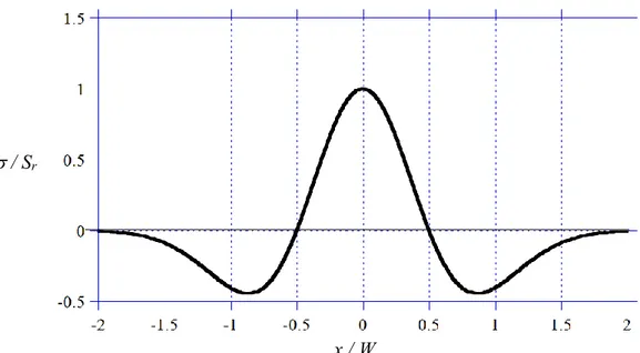
Weld residual stresses may be approximated by assuming a uniform stress distribution at the level of the yield strength of the material, which generally provide conservatively higher effect from weld residual stress when assessing a flaw at a weld. This assumption may be used for an initial assessment, but if not adequate safety margins are obtained, then more detailed information is needed about the distribution of the residual stresses through the component thickness. This appendix provide recommendations on distributions of residual stress in as-welded butt welds.
Weld residual stresses have large influence on degradation processes resulting in slow crack growth during operation, such as stress corrosion cracking or fatigue. However, the influence from residual stresses to failure by fracture is limited in some situations. There are numerical and experimental investigations showing a declining influence from weld residual stress on the driving force for fracture in ductile materials in situations with high primary loading (Lr > 0.8). The effect is due to substantial
plasticity at the crack front before initiation of fracture in these cases, and the effect is rapidly decreasing for lower Lr. ASME Section XI disregard weld residual stress in all situations for fracture of austenitic
stainless steels, but this approximation can be rough for situations dominated by secondary loads (e.g. weld residual stress and a thermal shock) or if the material is not sufficiently ductile. Procedures have been developed for consideration of the contribution from weld residual stresses at high Lr-values and
![Table R1. Coefficients for the 5 th order polynomial along the weld centreline [R1]](https://thumb-eu.123doks.com/thumbv2/5dokorg/3336847.18341/42.892.73.842.246.666/table-r-coefficients-th-order-polynomial-weld-centreline.webp)