Contents
1 Introduction 5
2 WiMAX technology 6
2.1 Why will WiMAX be a technology of the future? . . . 6
2.2 802.16d versus 802.16e . . . 7
3 Path loss models 8 3.1 Free space path loss . . . 8
3.2 Weissberger’s model . . . 9
3.3 Early ITU model . . . 9
3.4 Stanford University Interim (SUI) model . . . 10
4 Measurement campaign 12 4.1 Equipment . . . 12 4.1.1 Transmitter side . . . 12 4.1.2 Receiver side . . . 13 4.2 Measurement trip . . . 13 5 Measurement result 16 5.1 The collected data . . . 16
5.2 Mean with different window sizes . . . 16
5.3 Median with different window size . . . 17
5.4 Mode . . . 17
5.5 Standard deviation . . . 17
5.6 Histogram . . . 17
6 Data analysis 26 6.1 Free space path loss . . . 26
6.2 Weissberger’s model . . . 28
6.3 Early ITU model . . . 28
6.4 Standford University Interim model . . . 29
6.5 Discussion . . . 30 7 WRAP 31 7.1 Detvag-90/FOI . . . 31 7.2 WRAP measurement . . . 31 8 Summary 35 9 Reference 36
List of Figures
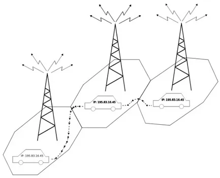
1 WiMAX scenario . . . 6
2 Block diagram at transmitter side . . . 12
3 The base station coupling. . . 13
4 Block diagram at the receiver antenna side . . . 14
5 The omni directional antenna with gain Gt=2.15 dBi. . . 14
6 The panel antenna CPA3320/34. . . 14
7 Mean diagrams . . . 19
8 Driven distance . . . 20
9 Driven path . . . 20
10 Median diagrams . . . 21
11 Mode diagram . . . 22
12 Standard deviation over mean . . . 22
13 Standard deviation over median . . . 23
14 Driven route . . . 23
15 Photos on the terrain . . . 24
16 Histogram over each of the antennas. . . 25
17 Free space path loss . . . 26
18 Weissberger’s model . . . 28
19 Early ITU model . . . 29
20 Standford University Interim model . . . 30
21 Map from the WRAP program . . . 32
22 Diagrams over terrain and magnitude . . . 33
23 WRAP prediction tool . . . 34
24 Receiver antenna . . . 37
List of Tables
1 WiMAX Parameters . . . 7
2 SUI Parameters . . . 11
3 Detvag-90 . . . 31
4 WRAP color magnitude . . . 32
Abstract
Propagation measurements at the frequency 3.5 GHz for the WiMAX tech-nology have been conducted. The purpose of these measurements is that a coverage analysis should be accomplished. The mathematical software pack-age MATLAB has been used to analyze the collected data from the measure-ment campaign. Path loss models have also been used and a comparison between these models and the collected data has been performed. An analysis prediction tool from an application called WRAP has also been used in the comparison with the collected data.
In this thesis, different receiver antennas have been used during the mea-surement campaign and the results have been compared.
Keywords: WiMAX, path loss models, omni directional antenna, panel antenna, mean, median, mode
1
Introduction
In this thesis, a study of propagation characteristics at frequencies of WiMAX technology and a coverage analysis in different environments was done. WiMAX technology standard 802.16e supports handover [15], which makes this standard to be interesting because it is possible to get WiMAX cover-age when going on a business trip by bus to give an example. With this technology, it is possible to use Internet without any connection loss because handover will take care of your connection when moving out from one base station cell to another base station cell.
The study was done with employing one base station antenna and one receiver antenna. Different receiver antennas were used. The receiver anten-nas propagation performance was compared with each other and an analysis was performed on the measured magnitude from different receiver antennas. A prediction and analysis tool, WRAP, and mathematical models were used on the measurement data. The measurement results were compared with theoretical path loss models.
This thesis is organized as follows: Chapter 2 introduce the WiMAX technology. In Chapter 3, some path loss models are described. In Chapter 4, the measurement campaign is explained and the equipment used for the measurement is introduced. In Chapter 5, an explanation of the measurement results and some analysis of the data collected at the measurement trip is done. In Chapter 6, the measured data results will be compared with the path loss models described in Chapter 3. In Chapter 7, results from the path loss prediction tool, WRAP is described. In Chapter 8, a conclusion of the thesis is presented.
2
WiMAX technology
The Worldwide Interoperability for Microwave Access (WiMAX) standard also known as IEEE 802.16 operates at 3.5 GHz. The propagation model for WiMAX follows the Line-of-sight (LOS) propagation which all signals over 30 MHz do and WiMAX use 3.5 GHz [2]. WiMAX is classified as a Wireless Metropolitan Area Network (WMAN). A Metropolitan Area Network is a network which is city wide and the WMAN is a network which is wireless and cover users in city wide ranges [6].
WiMAX is an interesting technology in Sweden since it has coming 1441 applications for the technology to the Swedish frequency provider, Post- och telestyrelsen (PTS). This will end in a auction because there are not as many available permissions as there are applications [11] [12]. One municipality in Sweden use an old permission and they will use it to let a power supply company use WiMAX to read the power consumption in the households.
Figure 1: This figure illustrate mobile WiMAX. A mobile part can move from one base station antenna in one cell into another cell with another base station antenna without connection loss.
2.1
Why will WiMAX be a technology of the future?
WiMAX can support many times better range than WiFi and this makes it possible for WiMAX to be used as WiFi with ranges which covers for
example a city instead of a caf´e. Sweden has the goal to make it possible for all inhabitant to connect to broadband. It is expensive to dig fiber cables to all households which lays miles away from each other. WiMAX can help Internet Service Providers (ISP’s) in Sweden to reach their goals. WiMAX ranges makes it fit good for these people who are living in rural areas and it will be cheaper for Sweden to let these households connect to Internet with WiMAX. This technology is also a good choice regarding the data rates which can reach transmission rates up to 75 Mbit/s [3] [6]. WiMAX does also support the MIMO (Multiple Input Multiple Output) antenna and Adaptive Antenna System (AAS) [4] [5]. The MIMO antenna can make it possible to reach higher data rates than WiMAX will be able to do with a Single Input Single Output (SISO) antenna. Higher data rates makes it possible to let a bigger number of multiple users connect to the same base station [1].
2.2
802.16d versus 802.16e
IEEE 802.16d (Fixed WiMAX) and IEEE 802.16e (Mobile WiMAX) are two known versions of 802.16. Fixed WiMAX fits big companies because it is not possible to move the mobile part out of range from the base station which it is connected to. With mobile WiMAX it is possible to move the mobile part out of range from the connected base station and still get connection to the Internet. This is possible because mobile WiMAX technology support seamless handovers. In this case, seamless handovers means that the same Internet Protocol (IP) address is used even if the mobile part is moving from one base stations cell to another base stations cell [7].
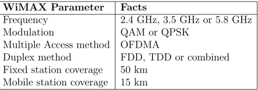
In the following table, some parameters specific for the WiMAX technol-ogy are presented [16] [17] [18].
Table 1: Some important parameters in the WiMAX technology. WiMAX Parameter Facts
Frequency 2.4 GHz, 3.5 GHz or 5.8 GHz
Modulation QAM or QPSK
Multiple Access method OFDMA
Duplex method FDD, TDD or combined Fixed station coverage 50 km
3
Path loss models
Path loss is about how much power the signal is reduced from the transmitter to the receiver antenna. There are different models to calculate the path loss and the models weighting different obstacles in the environment between transmitter and receiver antenna. Some theoretical models for path loss will be described in this chapter to let the reader be introduced to the models before studying them more in practice in Chapter 6.
3.1
Free space path loss
Free Space Path Loss (FSPL) is how much power the signal loses in the prop-agation from the sender antenna to the receiver antenna. FSPL depends on frequency and distance and the antenna type. There are two different types of antenna; isotropic antenna and non isotropic antenna, which has to be considered before calculating the FSPL. Isotropic antenna is a theoretical antenna which radiates equal power in all directions. The formula for calcu-lating FSPL with an isotropic antenna is [2]
Pt Pr = (4πd) 2 λ2 (1) where
Pt = Signal power at the transmitting antenna
Pr = Signal power at the receiver antenna
d = Propagation distance between antennas λ = Carrier wavelength
The carrier frequency λ can be calculated with the following formula λ = c
f (2)
where
c = Speed of light (3∗ 108 m/s)
f = Carrier frequency
The formula in (1) for the isotropic antenna is sometimes used to calculate approximations for the FSPL if the gain for the transmitter and receiver antenna are unknown. If the antenna type is known as nonisotropic antenna the most accurate FSPL will be retrieved with the following formula
Pt Pr = (4πd) 2 GrGtλ2 (3) where
Gr = Gain of the receiving antenna
Gt = Gain of the transmitting antenna
To get the FSPL in dB, use the following formula LdB = 10log
Pt
Pr
(4)
3.2
Weissberger’s model
This model uses the distance through vegetation that the signals has propa-gated when calculating the path loss. The formula to calculate the path loss with Weissberger’s model is [10][13]
L = ! 1.33f0.284d0.588 f if 14 < df ≤ 400 0.45f0.284d f if 0 < df ≤ 14 (5) where L = Path loss in dB f = Carrier frequency in GHz
df = Signals distance through vegetation in meter
Path loss will differ between 3 and 5 dB regarding the season. In the summer when trees got leaves, the path loss will be higher than in the winter when the trees are without leaves [13].
The Weissberger’s model can be applied to frequencies from 230 MHz to 95 GHz. This makes it possible to compare the WiMAX measurement at 3500 MHz with this model. The other condition for this model is that the model takes care of vegetation distances up to 400 meters.
3.3
Early ITU model
The early ITU model is another model that takes care of the signals distance through vegetation [10].
L = 0.2f0.3d0.6f (6)
L = Path loss
f = Frequency in GHz df = Depth of foliage
3.4
Stanford University Interim (SUI) model
There are two versions of the SUI model, one for signals around 2 GHz and one for other frequencies [8] [9]. The first formula presented here are for signals with a frequency around 2 GHz
L = A + 10γlog(d d0
) + s for d > d0 (7)
To compare the data simulation of the path loss model results with the results from the measurement campaign in this thesis, an extended formula will be used L = A + 10γlog(d d0 ) + Lf + Lh+ s (8) where A = 20log(4πd0 λ ) (9) γ = a− bhb+ c hb (10) Lf = 6.0log( f 2000) (11) Lh = ! −10.8log( hr
2000) for SUI Terrain Types A and B
−20.0log( hr
2000) for SUI Terrain Type C
where
d = Distance between antennas
d0 = The reference distance, 100 meter
s = A distributed factor between 8.2 dB and 10.6 dB λ = Carrier wavelength
hb = Height of the base station antenna
hr = Height of the receiver antenna
f = Carrier frequency in MHz
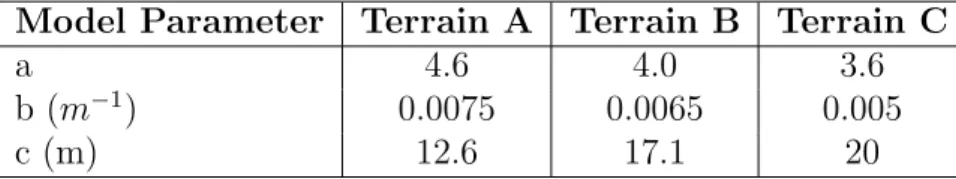
The parameters a, b and c in (10) are connected to the terrain type where the measurement campaign were done. Also the parameter Lh in the
extended formula depends on the environment. A reproduced table from [9] will be helpful to find out the correct values of the parameters.
Table 2: SUI parameters for different terrain.
Model Parameter Terrain A Terrain B Terrain C
a 4.6 4.0 3.6
b (m−1) 0.0075 0.0065 0.005
c (m) 12.6 17.1 20
The terrain type A is a terrain where it is difficult for the signal to propa-gate, for example it could be hilly, and this will result in maximum path loss. In contrast to A, terrain type C is a terrain where the signal can propagate easily and the signal reach the receiver with minimum path loss. The terrain type B is a mix of both terrain type A and terrain type C.
4
Measurement campaign
The equipment used for the measurement trip will first be presented in this chapter. How the collection of the measurement data has been done and under what circumstances will also be clarified in this Chapter. One of the purposes of the measurement campaign is that a test of the antennas in practice will be done. In Chapter 6, a data analysis will be performed to compare it with the results from the analysis of the measurement campaign which are purpose of the measurement analysis.
4.1
Equipment
Some equipments were used in the measurement campaign. In this section, the equipment will be presented and how they were connected to each other during the measurement campaign.
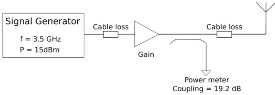
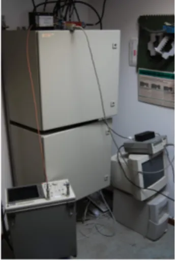
4.1.1 Transmitter side
A signal generator (HP8753D) at 3.5 GHz with a transmitter effect of 15 dBm to sending out the signal were used in the measurement campaign. There were a coupling at 19.2 dB to a power meter. The coupling at the trans-mitter side had a total cable loss of -2.0 dB. The sum of this were that the effective transmitter power through the base station antenna (panel antenna VP890/34) where at 34.65 dBm. In the Appendix A, a radiation pattern for this antenna is provided. Radiation pattern is an important characteristic when designing the network to know how to direct the antenna to get the main beam directed to the area with the highest capacity requirements and where the biggest amount of connection will be needed.
The transmitter antenna were mounted at a height of 40 m.
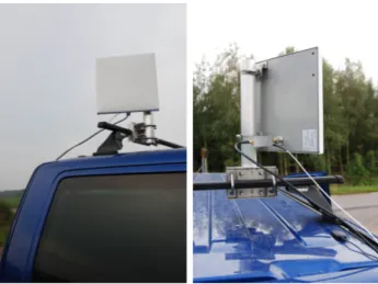
Figure 3: The base station coupling. 4.1.2 Receiver side
On the receiver side three different antennas (two omni directional antennas; one quarterwave antenna with 2.15 dBi and an antenna named VO8/34 with 8 dBi, a panel antenna CPA3320/34) where used. Two preamplifiers at 30 dB and 25 dB respectively were used in the measurement campaign. After these preamplifiers, a spectrum analyzer (HP8563E) were used. The cable loss at the receiver side is -4 dB. The receiver antenna were mounted at the roof of the van used for the measurement trip which were at a height of approximatly 2 m.
The car used in the measurement campaign had a cruise control which were helpful to get stable speed and measurement points with regular dis-tances.
The spectrum analyzer were able to take 8-10 measurements each second but the computer were the bottleneck in this part of the system which were able to register 5-10 measurement samples each second.
4.2
Measurement trip
The collected data consists of many shorter trips and a couple of longer trips. We used all three receiver antennas on the same stretch. Why driving the same stretch with different antennas were because the different antennas would be compared with each other. The antennas used at this stretch were two different omni antennas (quarterwave antenna with 2.15 dBi and VO8/34) and one panel antenna (CPA3320/34).
Figure 4: Block diagram of the receiver side. The total cable loss at this side is 4 dB.
Figure 5: The omni directional antenna with gain Gt=2.15 dBi.
Figure 6: The panel antenna CPA3320/34.
each of the antennas to see how stable each of the antennas were. The other reason for this scenario was to study if there are any difference between the antennas.
The same three antennas were used at an old measurement campaign which my supervisor at the company did before the thesis started. The main part of the measurement result were done when it were about 20◦C and
5
Measurement result
Data from the measurements were analyzed with help of MATLAB. When analyzing the data some different ways to get a good approximation of the mean value for the received signal where used. The different methods used to calculate the mean with a window size of different number of wavelengths, median and mode 1 where used.
5.1
The collected data
The collected data consisted of a time column and a column with the position from the GPS represented with a longitude and a latitude coordinate. The GPS updated its position ones per second. The GPS sent a signal with velocity, course and if the GPS were fix, which means if the GPS have been updated since last registration of measurement sample. In the data sheet, a flag was set every time the GPS updated the positions. The frequency were registered from the signal generator. To the data collection there were a column with the power amplitude which the spectrum analyzer registered. The spectrum analyzer registered 8-10 values per second.
5.2
Mean with different window sizes
The mean formula used to analyze the measurement results is [14] m = 1 n n " i=1 xi (12) where
n = Number of samples in the sum i = Measurement sample index number xi = Measured power magnitude
Only values from the past and the current value where used in this method. This makes the mean value to be unreliable in the start.
The mean curve in the diagrams with window size 100 and 200 wave-lengths, it can be seen that the curve fluctuate much in Figure 7. Compare these curves with the diagram with window size 300 wavelengths. The last diagram have to small fluctuations. The conclusion from this is that a win-dow size with 250 wavelengths should be the best alternative. This is also shown in Figure 7. The way driven can be seen in Figure 8 and in Figure 9.
5.3
Median with different window size
The median where used to see if it were possible to get a more accurate method to calculate a mean curve. Look at the diagrams where median are used in the Figure 10.
In simulation with the mean case which were described above, it is pos-sible to see that the diagram with the window size with 250 wavelengths is the most accurate window size.
5.4
Mode
Mode is the number that is represent most times of the values. In this report, only one diagram will be included just to show how it looks like. Why only one diagram is shown is because it not differs so much that it will be worth to show diagrams with different window sizes. When using mode to calculate the mean curve, the values received by the receiver antenna where rounded to an integer. See Figure 11 for mode diagram.
This diagram shows that the received magnitude fluctuate much and that there are not any values that are common to receive.
5.5
Standard deviation
To realize how accurate the mean in Figure 7 with 250 wavelengths is, stan-dard deviation were used. See Figure 12 for diagram over the stanstan-dard deviation with mean method and see Figure 13 over standard deviation with median as the mean method.
5.6
Histogram
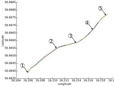
The antennas used on the same route have been studied and compared with each other. First, look at the Figure 14 to see how the GPS registered the route.
Some photos of the terrain against the base station antenna can be seen in Figure 15.
The plotted histograms for each measurements are shown in Figure 16. From the histograms it is possible to point out that the received signal with the omni directional antenna is varying most of these three measure-ments. For this antenna, the received signal is varying mostly between -60 dBm and -50 dBm.
When looking at the two measurements with the panel antenna, they are looking a bit different. The panel antenna which is not directed, focuses for
the received signals is around -60 dBm but looking at the panel antenna when it is directed, focus for the received signals is between -60dBm and -50dBm. When comparing the three measurements, similarities can be found between the two measurements with the panel antenna. With the omni directional antenna, almost no signals are received over -40 dBm.
(a) Th e wind ow size is 100 λ . (b ) The wi ndo w si ze is 200 λ . (c) The w ind ow si ze is 250 λ . (d ) The wi ndo w si ze is 300 λ . Figur e 7: Mean with w indo w size 100 , 200 , 250 and 300 w av elengths resp ectiv ely .
Figure 8: The distance between base station and the receiver antenna during one of the trips can be seen in this figure.
Figure 9: The path driven during the same trip as in Figure 8 can be seen in this figure.
(a) T he win do w size is 100 λ . (b ) The win do w size is 200 λ . (c) The w ind ow si ze is 250 λ . (d ) The win do w size is 300 λ . Figur e 10: Me dia n with windo w size 10 0, 20 0, 25 0, 300 w av eleng ths resp ec tiv ely .
Figure 11: Mode with window size 250 wave lengths. The blue plot is the magnitude received by the antenna and the red plot is the result of the mode.
Figure 12: The blue lines are the standard deviation, upper standard devi-ation and lower standard devidevi-ation and the red line is the mean with the window size 250 wavelengths.
Figure 13: The blue lines are the standard deviation, upper standard devia-tion and lower standard deviadevia-tion, and the red line is the average when using the median method with the window size 250 wavelengths.
Figure 14: Three different measurements. The blue line is the omni direc-tional antenna, the green line is the panel antenna and the red line is the panel antenna directed 20 degree. In this figure it is possible to see that the
Figure 15: Some photos at the terrain where the measurement with the different antennas were done.
(a) Histogram for omni directional antenna.
(b) Histogram for panel antenna.
(c) Histogram for panel antenna directed 20◦.
6
Data analysis
In this section, the mathematical path loss prediction models introduced in Chapter 3 will be applied and compared with the measurement results from the measurement campaign.
6.1
Free space path loss
One of the important path loss measurement is to compare the measurement campaign with the free space path loss. In Figure 17, it is possible to study the predicted path loss.
Figure 17: The cyan line is the received signal, the blue line is the actual path loss and the green line is the predicted free space path loss.
The line in cyan is the power in dBm registered by the spectrum analyzer. The green line is calculated by using the following formula
Pt
Pr
= (4πd)
2
and then the following formula to get the FSPL in dB. LdB = 10log
Pt
Pr
Both formulas where introduced in Chapter 3.1.
To get the blue line, the transmitted power where first calculated. The following calculations where used.
First it is necessary to know how much power were used to the power meter, which will be found with the following calculation
Pcoupled = 10−19.2/10= 0.012 = 1.2%
From this it is known that 1.2% power where used from the signal.
The power meter showed 15.5 dBm. The fact that the power meter use 19.2 dB realizes that the signal is
Signal = 15.5dBm + 19.2dB = 34.7dBm
The signal will be decreased with 2 dB cable loss, which will give the signal power to the antenna to be
Signal To Antenna = 34.7dBm− 2dB = 32.7dBm
The Signal To Antenna, which were just calculated, is the transmitted power from the base station.
To get the path loss from base station antenna to receiver antenna, the following calculation will be done for every measurement to compensate for the gain at 25 dB and 30 dB respectively and the 4 dB cable loss:
Magnitude Receiver Antenna = Registered Magnitude− 25dB + 4dB − 30dB Registered Magnitude is the power measured by the spectrum analyzer. To get the path loss which is illustrated by the blue line, the finally calculation is
Path Loss = (34.7dBm + 14.5 dBi)− Magnitude Receiver Antenna The antenna gain for the base station antenna where used in the final calcu-lation at 14.5 dBi.
The diagram shows that the free space path loss with the prediction tool is not as huge as the real measured path loss is.
Figure 18: The green line is the Weissberger’s predicted results. The cyan line is the measured results during the measurement trip and the blue line is the measures path loss.
6.2
Weissberger’s model
The Weissberger’s model takes care of the depth of foliage. In this prediction model, one third of the distance to the base station were used as the depth of foliage. The Figure 18 will show the results of this mathematical prediction tool.
If the distance through vegetation is longer than 400 meter, the distance will be set to 400 meter. The Weissberger’s model predicted much lower path loss than the real path loss was.
6.3
Early ITU model
Early ITU model is competiting with the Weissberger’s model. They both take care of the depth of foliage. In Figure 19, the result of the early ITU mathematical prediction tool is shown.
Figure 19: The green line is the early ITU predicted results. The cyan line is the measured results during the measurement trip and the blue line is the measures path loss.
were used. If the distance through vegetation is longer than 400 meter, the distance will be set to 400 meter. At these distances and at 3.5 GHz, this model is a more accurate method than Weissberger’s model, but the results are not satisfying.
6.4
Standford University Interim model
When predicted the path loss with the SUI model, the distributed factor at 10.6 dB where used. Terrain type C where used. The results is shown in Figure 20.
The interpretation of the SUI model gives the result closest to the mea-surement results.
Figure 20: The green line is the SUI model predicted results. The cyan line is the measured results during the measurement trip and the blue line is the measures path loss.
6.5
Discussion
The SUI model gave a predicted path loss closest to the measurement. All models applied in this thesis where optimistic and gave a predicted path loss better than the path loss from the measurement. A semi-terrain based model is needed and the ITU-R P.1546 is that kind of model [20].
The antennas used for the measurement trip had impact on the result as were showed in Chapter 5.6. The directed panel antennas received strong signals that the omni directional antenna could not receive.
7
WRAP
WRAP is a software used to plan how wireless networks will be designed. This software can be used for many things, for example to analyze measured data. In this report some analyzes with WRAP will be shown.
7.1
Detvag-90/FOI
Detvag-90/FOI is a prediction tool in WRAP for path loss. This model uses several propagation models and weight them to get the final prediction of the path loss. In Table 3, the different models used in the Detvag-90/FOI are arranged. The table are a part of a reproduced table from [19].
Table 3: Models in detvag-90.
Frequency range and Accuracy
Method Above 1000 MHz
Low High
Spherical earth None None
Diffraction Giovaneli GTD
No. of obstacles 3 7
Urban Add cover height Add cover height Vegetation Add cover height Add cover height
Effective antenna height None None
GTD in the table is short for Geometrical Theory of Diffraction. GTD and Giovaneli are two models used in the calculations to the detvag-90.
Spherical earth make an approximation of signals as direct, ground and surface waves and use them in calculations.
7.2
WRAP measurement
The data collected at the measurement campaign were included into the WRAP program.
In the map, the base station is marked out at east. The red areas are cities.
The driven path is in different colors. The colors represent different mag-nitude and follow Table 4.
From the driven path with magnitude in Figure 21, some diagrams were done. The WRAP program using maps with information about the terrain above sea which is the height where the car where placed and the receiver
Figure 21: The driven path with the magnitude on a map from the WRAP program.
Table 4: The colors corresponding magnitude.
Color Magnitude Blue 20 Light green 15 Yellow 10 Cyan 5 Dark green -5
Black outside range
antenna where placed on the roof of the car which gives the actual height where the receiver antenna where placed. In Figure 22, two diagrams are shown. In the first diagram, the black line which is filled with blue under it, is the height where the measurement where done above sea level. There are some other colors in this diagram. In Table 5, explanations to the colors can be found.
Figure 22: The diagram at the top is showing the terrain. The black line filled with blue under is the receiver antenna height above sea level. The colors corresponding to different terrain types. For further explanation, see Table 5.
Table 5: WRAP is using the following colors when representing different terrains.
Color Terrain Light green Pasture
Red Cities with more than 200 inhabitants Blue Hardwood forest/coniferous forest Yellow Cities with maximum 200 inhabitants Dark green Provinces with buildings
this magnitude with the distance to the base station, Figure 8 can be used. WRAP includes several propagation prediction tools. In this thesis, the propagation tool, Detvag-90/FOI, described in Chapter 7.1 were used. The result of this tool is shown in Figure 23.
The interpretation of Detvag-90/FOI were close to the measurements and it is a adequate approximation of how the signal will propagate.
Figure 23: The result when using WRAP prediction propagation tool, Detvag-90/FOI. The magnitude from the measured route is also visible in this figure.
8
Summary
When looking at the histograms, it is possible to make a conclusion that it is important to choose antenna and to direct the antenna as accurate as possible to get as much as possible out of the connection. In these measurements, the best choice of antenna where the directed panel antenna when it were directed, but even when it was not directed it were better than the omni directional antenna.
From the data analysis, the SUI model were the model which were closest to the measurements. The predicted propagation with the WRAP software gave results close to the measurement.
9
Reference
[1] Documentation from WiMAXPro.com, http://wimaxpro.com/
[2] William Stallings, Wireless Communications & Networks, Pearson Pren-tice Hall, 2005
[3]WiMAX, General information about the standard 802.16, Rohde & Schwarz
[4] WiMAX MIMO and AAS, ArrayComm Announces Network MIMO for
WiMAX, WiMAX Industry, November 21, 2005
[5] A. Salvekar, S. Sandhu, M-A. Voung and X. Qian, Multiple Antenna Technology in WiMAX Systems, Intel Technology Journal, vol. 08, Issue 03, pp 228-239, August 20, 2004
[6] Case Studies, Intel,http://www.intel.com/standards/case/case wimax.htm
[7] WiMAX information, NORDIC nowire, http://www.nowire.se/
[8] Fabricio Lira Figueiredo and Paulo Cardieri, Coverage Prediction and Performance Evaluation of Wireless Metropolitan Area Networks based on IEEE 802.16, Journal of communication and information systems, vol. 20, no. 3, pp 132-140, 2005
[9] V.S. Abhayawardhana, I.J. Wassell, D. Crosby, M.P. Sellars, M.G. Brown,
University of Cambridge, Comparison of Empirical Propagation Path Loss Models for Fixed Wireless Access Systems
[10] J. D. Parsons, The Mobile Radio Propagation Channel (Second Edition), John Wiley & Sons, 2000
[11] Mats Lewan, Telia vill bygga tradl¨ost bredband i varenda buske, Ny Teknik, no. 37, pp 18, September 13, 2006
[12] Jonas Karlsson, PTS v¨aljer auktion, Elektronik i norden, No. 16, pp 8, 2006
[13] IEEE Transactions on vehicular technology, Vehicular Technology Soci-ety, Volume 37, Number 1, February 1988
[14] Ekblom m.fl., Tabeller och formler for NV-programmet, Fj¨arde uppla-gan, Liber AB, 1997
[15] Thomas Zemen,WiMAX Standards History from 802.16 to 802.16e, The Telecommunications Research Center Vienna, November 22, 2006
[16] Information from WiMAX.com, http://www.wimax.com/education
[17] White papers, Intel
[18] WiMAX Broadband Wireless Technology Access, Intel [19] WRAP User Manual Introduction, WRAP, AerotechTelub
[20] E. ¨Ostlin, H. Suzuki and H-J. Zepernick, Evaluation of the Propagation Model Recommendation ITU-R P.1546 for Mobile Services in Rural Aus-tralia, April 28, 2006
Appendix A
Figure 24: This antenna were used as a receiver antenna in the measurement campaign.
Figure 25: This antenna were used as the base station antenna in the mea-surement campaign.