Umeå University
Department of mathematics and mathematical statistics
Directional edge detection by the gradient method
applied to linear and non-linear edges
Spring 2020
Course: Thesis Project for the Degree of Bachelor of Science in Mathematics, 15 credits Author: Mohammed Al-Dory
Abstract
When we humans look at images, especially paintings, we are usually interested in the sense of art and what we regard as “beauty”. This may include colour harmony, fantasy, realism, expression, drama, ordered chaos, contemplative aspects, etc.
Alas, none of that is interesting for a robot that processes a two-dimensional matrix representing what we humans call an image.
Robots, and other digital computers, are programmed to care about things like resolution, sampling frequency, image intensity, as well as edges. The detection of edges is a very important subject in the field of image processing. An edge in an image represents the end of one object and the start of another object. Thus, edges exist in different shapes and forms. Some edges are horizontal, other edges are vertical and there are also diagonal edges, all these edges are straight lines with constant slopes. Then we have also circular and curved edges whose slopes depend on the spatial variables. It is not always beneficial to detect all edges in an image, sometimes we are interested in edges in a certain direction. In this work we will explain the mathematics behind edge detection using gradient approach and try to give optimal ways to detect linear edges in different directions and discuss detection of non-linear edges. The theory developed in this work will then be applied and tested using Matlab.
Keywords: Edge detection, Gradient, Image processing, Computer vision, Circular convolution, Transform methods, Applied mathematics.
Sammanfattning
När vi människor tittar på bilder, särskilt målningar, är vi vanligtvis intresserade av konst- känslan och vad vi betraktar som “skönhet”. Detta inkluderar bl. a. färgharmoni, fantasi, realism, uttryck, drama, ordnat kaos, kontemplativa aspekter, osv.
Tyvärr är inget av detta intressant för en robot som behandlar en tvådimensionell matris som representerar vad vi människor kallar för bild.
Robotar, och andra digitala datorer, är programmerade för att bry sig om saker som: upplösning, samplingsfrekvens, bildstyrka samt kanter. Att detektera kanter är ett viktigt område inom bildbehandling. En kant i en bild innebär slutet på ett objekt och början på ett annat. Därför existerar kanter i olika slag. Vissa kanter är horisontella, andra kanter är vertikala och det finns också diagonala kanter, alla dessa kanter har former av räta linjer med konstanta lutningar. Dessutom finns det även cirkulära och böjda kanter vars lutningar beror på rumsvariablerna. Det är inte alltid välgörande att detektera alla kanter i en bild, ibland är vi endast intresserade av bilder i en viss riktning. I detta arbete kommer vi att gå genom matematiken bakom kantdetektering med gradientmetoden samt försöka ange optimala sätt att detektera linjära kanter i olika riktningar. Teorin som vi kommer att utveckla kommer därefter att tillämpas och testas med hjälp av Matlab.
Nyckelord: Kantdetektering, Gradient, Bildbehandling, Datorseende, Cirkulär faltning, Transformmetoder, Tillämpad matematik.
1
Content
1 Introduction ... 2 1.1 Mathematical definitions ... 2 1.1.1 The gradient ... 2 1.1.2 The Convolution ... 21.1.3 The Fourier transform ... 3
2 Theory ... 6
2.1 Images as functions and matrices ... 6
2.2 Edges ... 6
2.3 Filter design ... 7
2.3.1 Low-pass filters ... 8
2.3.2 High-pass filters ... 8
2.4 Applying filters to linear edges ... 8
2.4.1 Horizontal and vertical edges... 9
2.4.2 Diagonal edges ... 9
2.5 Noise in images ... 11
3 Results ... 14
3.1 Linear edges ... 14
3.1.1 Horizontal and vertical edges... 14
3.1.2 Diagonal edges ... 17
3.1.3 Technical issues with diagonal edges ... 21
3.2 Non-linear edges ... 24
3.3 Dealing with noise ... 25
4 Discussions and conclusions ... 28
5 Suggestions for future work ... 29
6 Appendices ... 30
2
1 Introduction
Edge detection is a wide subject in the field of computer vision and image processing. Computer scientists have been working out different approaches for efficient edge detection all of which are based upon mathematical principles of calculus and transform methods. Our aim in this work is to explain edge detection from a mathematical perspective using the gradient approach and apply it on linear and non-linear edges. Furthermore, the issue of noise and its effects on edge detection are explained. To proceed, we need some definitions.
1.1 Mathematical definitions
We present the mathematical tools needed to perform edge detection by the gradient approach. Since we are working with image processing, all continuous functions in this section are assumed to be defined as 𝑓: ℝ2 → ℝ, that is, scalar functions of two variables defined for all 𝑥, 𝑦 ∈ ℝ2. Furthermore, all discrete arrays are assumed to be matrices from the set 𝑀𝑚×𝑛(ℂ), i.e. the set of 𝑚 × 𝑛 matrices with complex entries.
1.1.1 The gradient
The gradient is a vector valued function whose vector field, at a point (𝑥, 𝑦), points in the direction of maximum change.
Definition 1.1 Given a function 𝑓: ℝ2 → ℝ, the gradient ∇𝑓(𝑥, 𝑦) is defined as
∇𝑓(𝑥, 𝑦) = (𝜕𝑓 𝜕𝑥,
𝜕𝑓
𝜕𝑦) 1.1
1.1.2 The convolution
The convolution is the amount of overlap between two functions 𝑓 and 𝑔 when the one is shifted over the other.
Definition 1.2 Let 𝑓(𝑥, 𝑦) and 𝑔(𝑥, 𝑦) be dimensional continuous signals, then the two-dimensional convolution may be given by the double integral
(𝑓 ∗ 𝑔) = ∫ ∫ 𝑓(𝜏𝑥, 𝜏𝑦) ∙ 𝑔(𝑥 − 𝜏𝑥, 𝑦 − 𝜏𝑦)𝜕𝜏𝑥𝜕𝜏𝑦 ∞ −∞ ∞ −∞ 1.2
Definition 1.3 For two-dimensional discrete signals, i.e. sampled images defined by matrices 𝑈, 𝑉 ∈ 𝑀𝑚×𝑛(ℂ), the convolution may be given by
(𝑈 ∗ 𝑉)𝑚×𝑛= ∑ ∑ 𝑈𝑖,𝑗∙ 𝑉𝑚−𝑖,𝑛−𝑗 ∞ 𝑗=−∞ ∞ 𝑖=−∞ 1.3
However, since digital images have finite size, we can define a circular convolution by first extending the finite signals periodically. That is, we say that for the 𝑚 × 𝑛 signal 𝑈 with components 𝑢𝑘,𝑙, we have 𝑢𝑘 𝑚𝑜𝑑 𝑚,𝑙 𝑚𝑜𝑑 𝑛. This means that the signal 𝑈 is extended periodically with period 𝑚 in the 𝑘 −direction and 𝑛 in the 𝑙 −direction. The same periodic extension holds for the 𝑚 × 𝑛 signal 𝑉. Now, if the two signals are convolved with each other, the result is the convolution 𝐶 = 𝑈 ∗ 𝑉 which, is the matrix 𝐶 ∈ 𝑀𝑚×𝑛(ℂ) with elements
3 𝑐𝑟,𝑠 = ∑ ∑ 𝑢𝑖,𝑗∙ 𝑣𝑟−𝑖,𝑠−𝑗 𝑛−1 𝑗=0 𝑚−1 𝑖=0 , 1.4 where 0 ≤ 𝑖 ≤ 𝑚 − 1 and 0 ≤ 𝑗 ≤ 𝑛 − 1.
Definition 1.4 The expression (1.4) is the circular convolution in two dimensions.
Remark 1.1. The periodicity of the extension of a 𝑚 × 𝑛 signal 𝑈 implies that for any integers 𝑖 and 𝑗 we have ∑ ∑ 𝑢𝑘,𝑙 𝑗+𝑛−1 𝑙=𝑗 𝑖+𝑚−1 𝑘=𝑖 = ∑ ∑ 𝑢𝑘 𝑚𝑜𝑑 𝑚,𝑙 𝑚𝑜𝑑 𝑛 𝑛−1 𝑙=0 = 𝑚−1 𝑘=0 ∑ ∑ 𝑢𝑘,𝑙 𝑛−1 𝑙=0 𝑚−1 𝑘=0
Remark 1.2. In many textbooks the linear convolutions in (1.2) and (1.3) are denoted by the symbol ∗ while the circular convolution is denoted by other symbols like ⊗ or ⋆. However, since the circular convolution is the standard for our work, it will be denoted by ∗.
1.1.3 The Fourier transform
When performing signal processing, it is often convenient to express signals as functions of frequency rather than functions of space (or time). One way to transform functions from the spatial domain into the frequency domain is to apply the Fourier transform. Here 𝜔1 and 𝜔2 are frequency variables.
Definition 1.5. For a continuous function 𝑓: ℝ2 → ℝ, the two-dimensional Fourier transform is given by 𝐹̂(𝜔1, 𝜔2) = ℱ{𝑓(𝑥, 𝑦)} = ∫ ∫ 𝑓(𝑥, 𝑦)𝑒−𝑖(𝜔1𝑥+𝜔2𝑦)𝑑𝑥𝑑𝑦 ∞ −∞ ∞ −∞ 1.5 we have also
Definition 1.6. The two-dimensional inverse Fourier transform may be given by
𝑓(𝑥, 𝑦) = ℱ−1{𝐹̂(𝜔1, 𝜔2)} = ∫ ∫ 𝐹̂( 𝜔1, 𝜔2)𝑒𝑖(𝜔1𝑥+𝜔2𝑦)𝑑𝜔1𝑑𝜔2 ∞ −∞ ∞ −∞ 1.6
For a discrete 2D matrix, we define the two-dimensional discrete Fourier transform, or DFT. Definition 1.7. For a matrix 𝐴 ∈ 𝑀𝑚×𝑛(ℂ), the DFT, is the matrix 𝐴̂ ∈ 𝑀𝑚×𝑛(ℂ) with components 𝑎̂𝑘,𝑙= ∑ ∑ 𝑎𝑘,𝑙𝑒−2𝜋𝑖( 𝑘𝑟 𝑚+ 𝑙𝑠 𝑛) 𝑛−1 𝑠=0 𝑚−1 𝑟=0 1.7 We also have
4 Definition 1.8. If 𝐴̂ ∈ 𝑀𝑚×𝑛(ℂ) is the matrix with components 𝑎̂𝑘,𝑙 given by (1.7), then the two-dimensional inverse discrete Fourier transform, or IDFT, is the matrix 𝐴 ∈ 𝑀𝑚×𝑛(ℂ), with components 𝑎𝑘,𝑙 = 1 𝑚𝑛 ∑ ∑ 𝑎̂𝑘,𝑙𝑒 2𝜋𝑖(𝑘𝑟𝑚+𝑙𝑠𝑛) 𝑛−1 𝑠=0 𝑚−1 𝑟=0 1.8
One of the useful properties of the Fourier transform is that it turns a convolution in the time/spatial domain into a multiplication in the frequency domain.
Theorem 1.1 (The convolution theorem for two-dimensional discrete signals) Suppose that we have two matrices 𝑈 ∈ 𝑀𝑚×𝑛(ℂ) and 𝑉 ∈ 𝑀𝑚×𝑛(ℂ) with (two-dimensional) DFTs 𝑈,̂ 𝑉̂ ∈ 𝑀𝑚×𝑛(ℂ) consisting of components given by equation (1.7), i.e.
𝑢̂𝑘,𝑙 = ∑ ∑ 𝑢𝑘,𝑙𝑒−2𝜋𝑖(𝑘𝑟𝑚+ 𝑙𝑠 𝑛) 𝑛−1 𝑠=0 𝑚−1 𝑟=0 and 𝑣̂𝑘,𝑙= ∑ ∑ 𝑣𝑘,𝑙𝑒−2𝜋𝑖( 𝑘𝑟 𝑚+ 𝑙𝑠 𝑛) 𝑛−1 𝑠=0 𝑚−1 𝑟=0 respectively.
Then 𝐶 = 𝑈 ∗ 𝑉 has (two-dimensional) DFT 𝐶 ∈ 𝑀𝑚×𝑛(ℂ) with elements
𝑐̂𝑘,𝑙 = 𝑢̂𝑘,𝑙∙ 𝑣̂𝑘,𝑙 1.9 for 0 ≤ 𝑘 ≤ 𝑚 − 1 and 0 ≤ 𝑙 ≤ 𝑛 − 1. Proof 1: By (1.7), 𝑐̂𝑘,𝑙 is given by 𝑐̂𝑘,𝑙 = ∑ ∑ 𝑐𝑘,𝑙𝑒−2𝜋𝑖( 𝑘𝑟 𝑚+ 𝑙𝑠 𝑛) 𝑛−1 𝑠=0 𝑚−1 𝑟=0 and by (1.4), 𝑐𝑟,𝑠 is given by 𝑐𝑟,𝑠 = ∑ ∑ 𝑢𝑥,𝑦∙ 𝑣𝑟−𝑥,𝑠−𝑦 𝑛−1 𝑦=0 𝑚−1 𝑥=0
substituting this expression in the formula for 𝑐̂𝑘,𝑙 above and interchanging the summation order yield 𝑐̂𝑘,𝑙 = ∑ ∑ 𝑐𝑘,𝑙𝑒−2𝜋𝑖( 𝑘𝑟 𝑚+ 𝑙𝑠 𝑛) 𝑛−1 𝑠=0 𝑚−1 𝑟=0 = ∑ ∑ ( ∑ ∑ 𝑒−2𝜋𝑖(𝑘𝑟𝑚+ 𝑙𝑠 𝑛) 𝑛−1 𝑠=0 𝑚−1 𝑟=0 ) 𝑢𝑥,𝑦∙ 𝑣𝑟−𝑥,𝑠−𝑦 𝑛−1 𝑦=0 𝑚−1 𝑥=0
In the 𝑟 and 𝑠 sums, define 𝑝 = 𝑟 − 𝑥,and 𝑞 = 𝑠 − 𝑦 (so that 𝑟 = 𝑥 + 𝑝 and 𝑠 = 𝑦 + 𝑞) and change the summation limits accordingly to find
𝑐̂𝑘,𝑙 = ∑ ∑ ( ∑ ∑ 𝑒 −2𝜋𝑖(𝑘(𝑥+𝑝)𝑚 +𝑙(𝑦+𝑞)𝑛 ) 𝑛−1−𝑦 𝑞=−𝑦 𝑚−1−𝑥 𝑝=−𝑥 ) 𝑢𝑥,𝑦∙ 𝑣𝑝,𝑞 𝑛−1 𝑦=0 𝑚−1 𝑥=0
5 = ( ∑ ∑ 𝑢𝑥,𝑦𝑒−2𝜋𝑖(𝑘𝑥𝑚+ 𝑙𝑦 𝑛) 𝑛−1 𝑦=0 𝑚−1 𝑥=0 ) ( ∑ ∑ 𝑣𝑝,𝑞𝑒−2𝜋𝑖(𝑘𝑝𝑚+ 𝑙𝑞 𝑛) 𝑛−1−𝑦 𝑞=−𝑦 𝑚−1−𝑥 𝑝=−𝑥 ).
Now, exploit the fact that the term 𝑣𝑝,𝑞𝑒−2𝜋𝑖(
𝑘𝑝 𝑚+
𝑙𝑞
𝑛) is periodic in 𝑝, 𝑞, by remark (1.1), we can
shift the summation limits into 𝑝 = 0 to 𝑚 − 1 and 𝑞 = 0 to 𝑛 − 1. Which gives
𝑐̂𝑘,𝑙 = ( ∑ ∑ 𝑢𝑥,𝑦𝑒−2𝜋𝑖( 𝑘𝑥 𝑚+ 𝑙𝑦 𝑛) 𝑛−1 𝑦=0 𝑚−1 𝑥=0 ) ( ∑ ∑ 𝑣𝑝,𝑞𝑒−2𝜋𝑖( 𝑘𝑝 𝑚+ 𝑙𝑞 𝑛) 𝑛−1 𝑞=0 𝑚−1 𝑝=0 ) = 𝑢̂𝑘,𝑙 ∙ 𝑣̂𝑘,𝑙.
This proves the theorem.
□
Suppose that we have signals 𝐴, 𝐵, 𝐶 ∈ 𝑀𝑚×𝑛(ℂ), where 𝐶 = 𝑝𝐴 + 𝑞𝐵, for some constants 𝑝, 𝑞 ∈ ℂ, so that 𝑐𝑘,𝑙 = 𝑝𝑎𝑘,𝑙+ 𝑞𝑏𝑘,𝑙. Then, by definition (1.7), the Fourier transform of 𝐶 is the matrix 𝐶̂ ∈ 𝑀𝑚×𝑛(ℂ) with components𝑐̂𝑘,𝑙 = ∑ ∑ 𝑐𝑘,𝑙𝑒−2𝜋𝑖( 𝑘𝑟 𝑚+ 𝑙𝑠 𝑛) 𝑛−1 𝑠=0 = ∑ ∑(𝑝𝑎𝑘,𝑙+ 𝑞𝑏𝑘,𝑙)𝑒−2𝜋𝑖( 𝑘𝑟 𝑚+ 𝑙𝑠 𝑛) 𝑛−1 𝑠=0 𝑚−1 𝑟=0 𝑚−1 𝑟=0
Rearranging the term on the right-hand side gives
𝑐̂𝑘,𝑙 = 𝑝 ∑ ∑ 𝑎𝑘,𝑙𝑒−2𝜋𝑖( 𝑘𝑟 𝑚+ 𝑙𝑠 𝑛)+ 𝑞 ∑ ∑ 𝑏𝑘,𝑙𝑒−2𝜋𝑖( 𝑘𝑟 𝑚+ 𝑙𝑠 𝑛) 𝑛−1 𝑠=0 𝑚−1 𝑟=0 𝑛−1 𝑠=0 𝑚−1 𝑟=0 = 𝑝𝑎̂𝑘,𝑙+ 𝑞𝑏̂𝑘,𝑙 1.10
which means that
𝐶̂ = 𝑝𝐴̂ + 𝑞𝐵̂ 1.11
This property is called the linearity property. It says that the Fourier transform of a linear combination is the linear combination of the Fourier transforms.
6
2 Theory
2.1. Images as functions and matrices
In the analog case we regard the intensity of an image as a function 𝑓: ℝ2 → ℝ. Similarly, for discrete sampled images, the image intensity is represented by a matrix 𝐴 ∈ 𝑀𝑚×𝑛(ℂ) whose components 𝑎𝑖,𝑗, 0 ≤ 𝑖 ≤ 𝑚 − 1, 0 ≤ 𝑗 ≤ 𝑛 − 1, are the image pixels.
The term 𝑎0,0, indicates the pixel in the top-left corner of the image. So, if we consider the pixel 𝑎𝑖,𝑗, then the pixel 𝑎𝑖+1,𝑗 is the one just below 𝑎𝑖,𝑗. Similarly, the pixel 𝑎𝑖,𝑗+1 is the pixel to the right of 𝑎𝑖,𝑗. To summarise:
In the discrete case, the i-axis corresponds to the y-axis in the analog case, and the j-axis corresponds to the x-axis.
This fact is very important for understanding the upcoming results in this essay, especially for understanding the direction of edges to be detected, as we will see later.
2.2. Edges
Edges in images are the limits between objects, for an analog image whose intensity is given by a function 𝑓(𝑥, 𝑦), edges are regarded as the abrupt changes in the intensity of the image. So, we’d expect edges to occur where the gradient magnitude ‖𝑓(𝑥, 𝑦)‖ is large enough. For a discrete sampled image, we have a matrix whose components indicate pixels given by numerical values. Let 𝐴 ∈ 𝑀𝑚×𝑛(ℂ) be a matrix which represents a sampled image with pixels 𝑎𝑖,𝑗, 0 ≤ 𝑖 ≤ 𝑚 − 1, 0 ≤ 𝑗 ≤ 𝑛 − 1, Then for any integers 𝑘 and 𝑙:0 ≤ 𝑖 + 𝑘 ≤ 𝑚 − 1, 0 ≤ 𝑗 + 𝑙 ≤ 𝑛 − 1, we have an edge whenever |𝑎𝑖+𝑘,𝑗+𝑙− 𝑎𝑖,𝑗| is sufficiently large. In grayscale, lower values represent pixels with dark colour (0 = black), while higher values represent brighter pixels (255 = white). Consider figure 2.1 below, we have a 6 × 7 image denoted by 𝐴 with pixels having different values, we would expect to have an edge between the pixels 𝑎0,0 and 𝑎0,1 because the difference between the values is relatively large, however, we wouldn’t expect to see an edge between 𝑎0,0 and 𝑎1,0. If we highlight all places where there occur abrupt changes in the pixel values, we get the picture shown in figure 2.2.
7 Figure 2.1: A simple 6 × 7 image 𝐴 with valued pixels.
Figure 2.2: Image 𝐴 with highlighted edges.
The edges in figure 1.2 are not perfectly accurate. For instance, the edge between 𝑎1,2 and 𝑎1,3 should be clearer than the edge between 𝑎5,4 and 𝑎5,5 since |𝑎1,2− 𝑎1,3| > |𝑎5,4− 𝑎5,5|. This is just an example to give a basic idea of how edges are made of abrupt jumps in the image intensity.
What was done in the example above is edge detection by inspection. This approach is not efficient for large images with high resolution and complicated edges. To deal with such images, we need to develop a systematic way which, when applied to images, gives reliable results. One such way is filter design.
2.3. Filter design
Filters are very useful tools in signal/image processing. Given a sampled image represented by a matrix 𝐴 ∈ 𝑀𝑚×𝑛(ℂ), we can create another matrix (filter) 𝐵 ∈ 𝑀𝑚×𝑛(ℂ) which gives us a
8 desired effect on 𝐴. The effect is made by convolving the two matrices, i.e. by taking (𝐴 ∗ 𝐵) according to (1.4), resulting in a new matrix 𝐶 ∈ 𝑀𝑚×𝑛(ℂ) which is based on 𝐴 but carries the desired properties caused by 𝐵. For example, 𝐴 could represent a blurry image with unclear edges, so we want to design a filter 𝐵 to improve the edges in 𝐴 and the result is an image 𝐶 which is the same image as in 𝐴 but with clear edges. How to design the filter 𝐵 is the task in this case, it completely depends on what action we want it to make on 𝐴.This is what makes the subject of filter design a very vast one.
A two-dimensional filter, i.e. a filter defined as a matrix, is usually called a mask. 2.3.1 Low-pass filters
A low-pass filter is a filter which, in the frequency domain, cuts off components with frequencies higher than a certain threshold and only preserves components with lower frequencies. One such filter may be defined, in one-dimension, as
𝐿̂(𝜔) = {1, |𝜔| < 𝜔𝑡ℎ
0, 𝑒𝑙𝑠𝑒 2.1
Here, 𝜔𝑡ℎ is the threshold. In general, a low-pass filter satisfies the condition: lim
|𝜔|→∞𝐿̂(𝜔) = 0 2.3.2 High-pass filters
A high-pass filter is a filter which cuts off components with frequencies lower than a specified threshold. One such filter may be defined, in one-dimension, as
𝐻̂(𝜔) = {1, |𝜔| > 𝜔𝑡ℎ
0, 𝑒𝑙𝑠𝑒 2.2
In general, a high-pass filter satisfies the condition: 0 < lim
|𝜔|→∞|𝐻̂(𝜔)| < ∞
Remark 2.1. Note that if we have a function defined in the frequency domain as 𝐹̂(𝜔) = 1, for all 𝜔, then it follows that: 𝐻̂(𝜔) = 𝐹̂(𝜔) − 𝐿̂(𝜔) ⇔ 𝐿̂(𝜔) = 𝐹̂(𝜔) − 𝐻̂(𝜔). 𝐹̂(𝜔) is called “all-pass filter” since it preserves all components.
2.4 Applying filters to linear edges
Linear edges are edges that have the shape of straight lines with constant slopes. In an analog image represented by 𝑓(𝑥, 𝑦), a linear edge may be given by
𝑦 = 𝑘𝑥 + 𝑚 2.3
Where 𝑘, 𝑚 ∈ ℝ and 𝑘 is the slope of the edge. There are three types of linear edges: 1. Horizontal edges, where 𝑘 = 0 (parallel to the 𝑥 −axis).
2. Vertical edges, where k → ±∞ (parallel to the 𝑦 −axis). 3. Diagonal edges, where 𝑘 is finite and nonzero.
9 In this section we design filters that give ideal edge detections of the three cases listed above. 2.4.1 Horizontal and vertical edges2
Suppose that we have a discrete sampled image 𝐴 ∈ 𝑀𝑚×𝑛(ℂ) obtained by sampling an analog image given by 𝑓(𝑥, 𝑦), then 𝐴 has components 𝑎𝑟,𝑠= 𝑓(𝑥𝑠, 𝑦𝑟), where 𝑥𝑠 = 𝑠(∆𝑥) and 𝑦𝑟 = 𝑟(∆𝑦). Recall that edges are abrupt jumps in the values of 𝑓, in other words, where ‖𝛻𝑓(𝑥, 𝑦)‖ = ‖(𝜕𝑓
𝜕𝑥, 𝜕𝑓
𝜕𝑦)‖ is large. This could occur in one of the directions, in this case 𝜕𝑓 𝜕𝑥 and/or 𝜕𝑓
𝜕𝑦. If we consider only the 𝑦 −direction (that is 𝜕𝑓
𝜕𝑥 = 0), then, by our discussion in section 2.2, we would expect the difference 𝑓(𝑥𝑠, 𝑦𝑟) − 𝑓(𝑥𝑠, 𝑦𝑟−1) = 𝑎𝑟,𝑠− 𝑎𝑟−1,𝑠 to be large in magnitude. The expression ∆𝑓
∆𝑦=
𝑓(𝑥𝑠,𝑦𝑟)−𝑓(𝑥𝑠,𝑦𝑟−1)
𝑦𝑟−𝑦𝑟−1 in the discrete case corresponds to
𝜕𝑓 𝜕𝑦 in the analog case. It follows that
𝑎𝑟,𝑠− 𝑎𝑟−1,𝑠= 𝑓(𝑥𝑠, 𝑦𝑟) − 𝑓(𝑥𝑠, 𝑦𝑟−1) ≈ (∆𝑦) ∙ 𝜕
𝜕𝑦𝑓(𝑥𝑠, 𝑦𝑟) 2.4
Equation (2.4) shows that 𝑎𝑟,𝑠− 𝑎𝑟−1,𝑠 is approximately proportional to 𝜕
𝜕𝑦𝑓(𝑥𝑠, 𝑦𝑟), so for |𝑎𝑟,𝑠− 𝑎𝑟−1,𝑠| to be large, the term |𝜕
𝜕𝑦𝑓(𝑥𝑠, 𝑦𝑟)| must be large, which means we have large change of image intensity in the 𝑦 −direction. This implies detection of horizontal edges. Now, how do we obtain 𝑎𝑟,𝑠− 𝑎𝑟−1,𝑠 from 𝐴? Well, we design a filter (mask) which, when convolved with 𝐴, gives us 𝑎𝑟,𝑠− 𝑎𝑟−1,𝑠. The mask is 𝐻 ∈ 𝑀𝑚×𝑛(ℂ) with components ℎ0,0 = 1,
ℎ1,0 = −1, and all other ℎ𝑟,𝑠 = 0. Then, by (1.4), (𝐴 ∗ 𝐻)𝑟,𝑠 = 𝑎𝑟,𝑠− 𝑎𝑟−1,𝑠.
Similarly, to detect vertical edges, we search for abrupt changes in the 𝑥 −direction. We design a new mask 𝑉 ∈ 𝑀𝑚×𝑛(ℂ) with components 𝑣0,0 = 1, 𝑣0,1 = −1, and all other 𝑣𝑟,𝑠 = 0. Then (𝐴 ∗ 𝑉)𝑟,𝑠 = 𝑎𝑟,𝑠− 𝑎𝑟,𝑠−1= 𝑓(𝑥𝑠, 𝑦𝑟) − 𝑓(𝑥𝑠−1, 𝑦𝑟) and the equivalent of equation (2.4) for vertical edges is 𝑎𝑟,𝑠− 𝑎𝑟,𝑠−1 = 𝑓(𝑥𝑠, 𝑦𝑟) − 𝑓(𝑥𝑠−1, 𝑦𝑟) ≈ (∆𝑥) ∙ 𝜕 𝜕𝑥𝑓(𝑥𝑠, 𝑦𝑟) 2.5 where ∆𝑥 = 𝑥𝑟− 𝑥𝑟−1. 2.4.2 Diagonal edges
The discussion in the section 2.4.1 implies that the ideal way to detect a linear edge with slope 𝑘 is to search in the path of slope −1/𝑘. That is, we maximize the magnitude of the gradient ∇𝑓 by targeting the edge in a direction perpendicular to the edge.
Suppose we have an analog image 𝑓 and want to detect a linear diagonal edge in it. In this case we search for abrupt changes in both 𝑥 and 𝑦 directions. In the sampled image 𝐴, a diagonal edge with, say, slope 𝑘 = 1 is detected by convolving the image matrix 𝐴 with a mask defined as 𝐷1 with components 𝑑10,0 = 1, 𝑑11,1 = −1, and all other 𝑑1𝑟,𝑠 = 0. With this mask the convolution becomes (𝐴 ∗ 𝐷)𝑟,𝑠 = 𝑎𝑟,𝑠− 𝑎𝑟−1,𝑠−1= 𝑓(𝑥𝑠, 𝑦𝑟) − 𝑓(𝑥𝑠−1, 𝑦𝑟−1)
10 Since we seek for abrupt changes in both 𝑥 and 𝑦 directions, the equivalent of equation (2.4) is
|𝑎𝑟,𝑠− 𝑎𝑟−1,𝑠−1| ≈ ‖((∆𝑥) ∙ 𝜕
𝜕𝑥𝑓(𝑥𝑠, 𝑦𝑟), (∆𝑦) ∙ 𝜕
𝜕𝑦𝑓(𝑥𝑠, 𝑦𝑟))‖ 2.6
In general, for a sampled image 𝐴 ∈ 𝑀𝑚×𝑛(ℂ), the mask that gives ideal detection of a diagonal edge of positive slope 𝑘 =𝑎
𝑏∈ ℚ, where 0 < 𝑎 < 𝑛 and 0 < 𝑏 < 𝑚, may be defined as 𝐷 ∈ 𝑀𝑚×𝑛(ℂ) with components 𝑑0,0 = 1, 𝑑𝑏 ,𝑎= −1 and all other 𝑑𝑟,𝑠 = 0. The convolution, for positive 𝑘, is then given by
(𝐴 ∗ 𝐷)𝑟,𝑠 = 𝑎𝑟,𝑠− 𝑎𝑟−𝑏,𝑠−𝑎 = 𝑓(𝑥𝑠, 𝑦𝑟) − 𝑓(𝑥𝑠−𝑎, 𝑦𝑟−𝑏) 2.7
If the diagonal edge had a negative slope 𝑘 =𝑎
𝑏∈ ℚ, where 0 < 𝑎 < 𝑛 and 0 < 𝑏 < 𝑚, then the mask may be defined as 𝐷 ∈ 𝑀𝑚×𝑛(ℂ) with components 𝑑0,𝑛−1 = 1, 𝑑|𝑏| ,𝑛−1−|𝑎| = −1 and all other 𝑑𝑟,𝑠 = 0. The convolution, for negative k, is then given by
(𝐴 ∗ 𝐷)𝑟,𝑠 = 𝑎𝑟,𝑠− 𝑎𝑟−𝑏,𝑠+𝑎 = 𝑓(𝑥𝑠, 𝑦𝑟) − 𝑓(𝑥𝑠+𝑎, 𝑦𝑟−𝑏) 2.8 For equation (2.7), where 𝑘 is positive, The straight line between pixel 𝑎𝑟,𝑠 and pixel 𝑎𝑟−𝑏,𝑠−𝑎 has slope −𝑏
𝑎 = − 1
𝑘. Which is the path perpendicular to that of slope 𝑘 = 𝑎
𝑏. Similarly, For equation (2.8), where 𝑘 is negative, The straight line between pixel 𝑎𝑟,𝑠 and pixel 𝑎𝑟−𝑏,𝑠+𝑎 has slope −𝑏
𝑎= − 1
𝑘. Which is the path perpendicular to that of slope 𝑘 = 𝑎
𝑏. Therefore, in both the cases above the mask 𝐷 will give a search in the direction perpendicular to that of the edge, as will be seen in section 3.1.2.
However, sometimes we get across edges with slopes 𝑘 =𝑎
𝑏∈ ℚ, where |𝑎| and/or |𝑏| are greater than 𝑛 and 𝑚 respectively. For example, when there is a linear edge with slope
𝑘 = ±106 inside a 700 × 600 image matrix. In this case, |𝑎| = 106 > 600, so to detect this edge we simply treat it as a vertical edge, since |𝑘| is relatively large that the edge “looks” vertical. Similarly, if the edge was of slope 𝑘 = ±10−6, then |𝑏| = 106 > 700 and the magnitude of the slope is small enough for us to treat the edge as a horizontal edge.
There is also the case where the slope is not very large/small in magnitude but still is given by 𝑘 =𝑎
𝑏∈ ℚ, where 𝑎 > 𝑛 and 𝑏 > 𝑚. For example, when the edge has slope 𝑘 = ± 85431 54653 ≈ ±1.5631, inside a 700 × 600 image matrix. In this case both 𝑎 and 𝑏 surpass the image limits but the quotient is still not very large (small) in magnitude for us to treat the edge as a vertical (horizontal) edge. What we do instead is that we find another rational number 𝑘′= 𝑎′
𝑏′,
where 0 < 𝑎′ < 𝑛 and 0 < 𝑏′ < 𝑚, such that, 𝑎′ 𝑏′ ≈
𝑎
𝑏= 𝑘. For our example we can take |𝑎′| = 39 and |𝑏’| = 25, then |𝑘′| = |39
25| = |1.56| ≈ | 85431
54653|, and the mask 𝐷 can now be constructed, according to the models given above, using 𝑎’ and 𝑏’ depending on whether 𝑘’ is positive or negative.
Note that this also can apply to linear edges with irrational slopes, for example, if 𝑘 = ±𝜋, then the slope can be approximated using 𝑘′ = ±22
7, or ± 355
11 2.5 Noise in images
Noise in a digital image is an error added to the sampled image. It could be added during sampling of the analog image or during transmission of the sampled image. In any case, let 𝐵 ∈ 𝑀𝑚×𝑛(ℂ) represent a noisy image obtained by adding noise to a sampled image represented by 𝐴 ∈ 𝑀𝑚×𝑛(ℂ), then the two images are related by
𝐵 = 𝐴 + 𝐸 2.9
where 𝐸 ∈ 𝑀𝑚×𝑛(ℂ) is the matrix carrying the noise. The pixels of 𝐵 are then given by
𝑏𝑖,𝑗= 𝑎𝑖,𝑗+ 𝑒𝑖,𝑗 2.10
In figure 2.3(a) we see a sampled image3, we then add random noise to it and get the noisy image in figure 2.3(b). It appears clearly how noise decreases the image quality, one of the most significant aspects of this is how edges are harmed due to noise. So, we’d expect to have difficulties trying to find abrupt changes in a noisy image. Noise is seen to be caused by high-frequency energy, so to remove it, we use a low-pass filter. One such filter is the so called “nine-averaging mask 4” defined as 𝐷 ∈ 𝑀
𝑚×𝑛(ℂ) with components 𝑑𝑟,𝑠 = {
1
9, 𝑟, 𝑠 ∈ [−1,0,1]
𝑥, 𝑒𝑙𝑠𝑒 . This mask is periodically extended, which means that
𝑑𝑚−𝑖,𝑛−𝑗 = 𝑑−𝑖,−𝑗. Thus, by equation (1.4), the convolution (𝐵 ∗ 𝐷) consists of components (𝐵 ∗ 𝐷) 𝑘,𝑙 given by (𝐵 ∗ 𝐷)𝑘,𝑙 = 1 9(𝑏𝑘−1,𝑙−1+ 𝑏𝑘−1,𝑙+ 𝑏𝑘−1,𝑙+1 +𝑏𝑘,𝑙−1+ 𝑏𝑘,𝑙 + 𝑏𝑘,𝑙+1 +𝑏𝑘+1,𝑙−1+ 𝑏𝑘+1,𝑙+ 𝑏𝑘+1,𝑙+1)
This shows that the effect of convolving the image 𝐵 with the nine-averaging mask 𝐷 is summing up the values of pixel 𝑏𝑖,𝑗 and all eight pixels around it and then dividing by 9, hence the name “nine-averaging”.
Figure 2.4 shows the effect of 𝐷 on the noisy image 𝐵 in figure 2.3, the filtering is carried out once in figure 2.4 (a) and five times in (b). It is clear that the five times filtered image has poorer edges than the image filtered once, this is due to the fact that 𝐷, being a low-pass filter, cuts off high-frequency components, and since edges are high-frequency changes in the image intensity, they get filtered away the more 𝐷 is applied to the image.
The magnitude of the DFT of 𝐷, i.e.|𝐷̂|, is shown in figure 2.5, we see |𝐷̂| around origin in the frequency domain. Now, by theorem 1.1, the convolution (𝐵 ∗ 𝐷) in the spatial domain corresponds to multiplication 𝐵̂ ∙ 𝐷̂ (component by component) in the frequency domain. This means, as the shape of |𝐷̂| indicates, that the components with frequencies away from the origin (high-frequency components) are multiplied by low values and thus damped out, while the components close to the origin (low-frequency components) are multiplied by higher values and thus highlighted. See figure 2.5.
12
(a) (b)
Figure 2.3: (a): Original sampled image. (b): Noisy image.
(a) (b)
13 Figure 2.5: Plot of the magnitude of the DFT of the mask 𝐷.
14
3 Results
3.1 Linear Edges
3.1.1 Horizontal and vertical edges
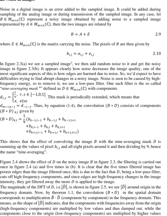
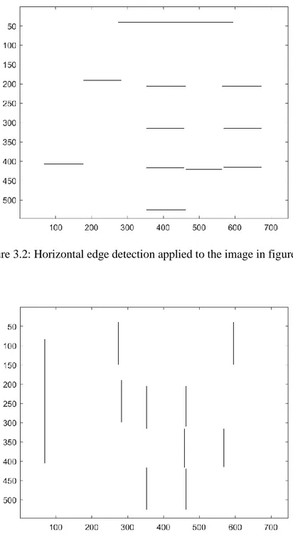
Consider the image shown in figure 3.1. It is a simple binary image with only vertical and horizontal edges, let this image be denoted by 𝐴. We attempt to detect the edges by applying the masks 𝐻 and 𝑉 defined in 2.4.1. Plotting the matrix |𝐴 ∗ 𝐻| gives the image shown in figure 3.2 below. As expected, only horizontal edges are detected whereas vertical edges are neglected. Similarly, if we plot |𝐴 ∗ 𝑉|, the result is the image in figure 3.3, which shows detection of vertical edges of the same image 𝐴.
The images in figures 3.2 and 3.3 are plotted in reverse order to make edges black against white background, which is more convenient when having a simple and undetailed image.
The two results are then combined by taking √|𝐴 ∗ 𝐻|2+ |𝐴 ∗ 𝑉|2, with this operation performed component by component. The new result is the image containing both the horizontal and the vertical edges, see figure 3.4.
15 Figure 3.2: Horizontal edge detection applied to the image in figure 3.1.
16 Figure 3.4: Both horizontal and vertical edges of the image in figure 3.1.
The two masks 𝐻 and 𝑉 are high-pass masks, thus they capture high-frequency components. To see the behaviour of these masks in the frequency domain, both the magnitudes of the DFTs of the two masks, i.e. |𝐻̂| and |𝑉̂|, are plotted around origin in figure 3.5. We see that |𝐻̂| has a constant form along the 𝑘 −axis and a form of a negative parabola along the 𝑙 −axis. Here the 𝑘 −axis corresponds to the 𝑦 −axis, so |𝐻̂| preserves high-frequency components along the 𝑦 −axis and thus captures horizontal abrupt changes, whereas along the 𝑙 −axis, which corresponds to the 𝑥 −axis, |𝐻̂| actually works as a low-pass mask since it vanishes away from origin, so along the 𝑥 −axis, |𝐻̂| does not preserve high-frequency components and thus the vertical edges are neglected. Recall that, by theorem 1.1, the convolution in the spatial domain corresponds to multiplication in the frequency domain, the convolution (𝐴 ∗ 𝐻) in the spatial domain becomes 𝐴̂ ∙ 𝐻̂ in the frequency domain. This implies that the edges in 𝐴, when convolved with 𝐻, are highlighted along the 𝑥 −axis (horizontal edges) whereas the vertical edges are neglected.
Similarly, |𝑉̂| is constant along the 𝑙 −axis and has a negative parabolic shape along the 𝑘 −axis, thus when multiplied by 𝐴̂, it highlights only vertical edges and neglects horizontal edges. See figure 3.5.
17
(a) (b)
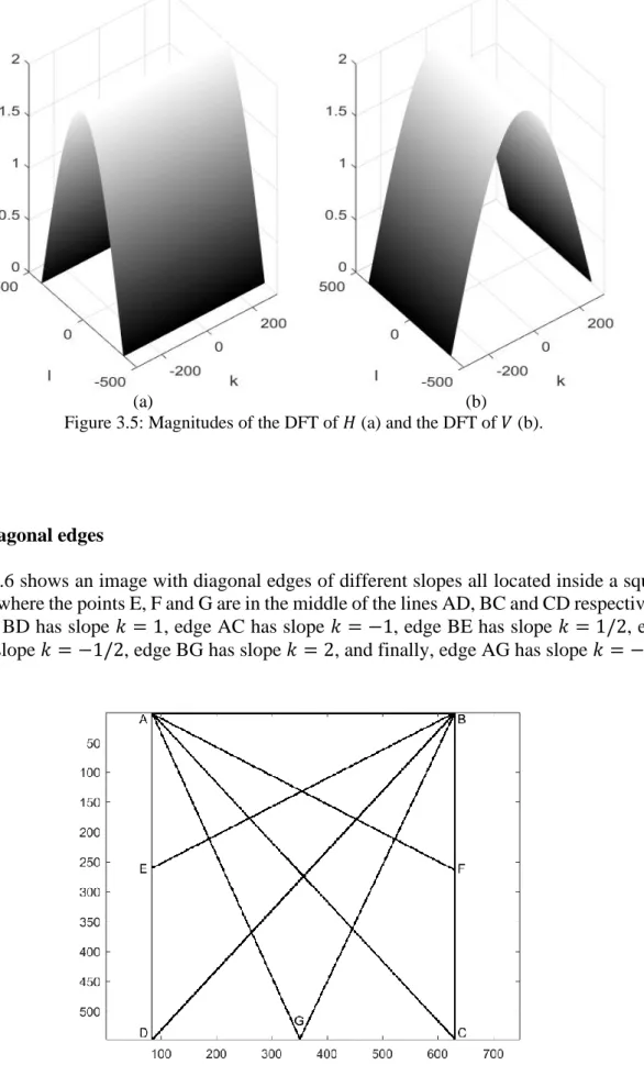
Figure 3.5: Magnitudes of the DFT of 𝐻 (a) and the DFT of 𝑉 (b).
3.1.2 Diagonal edges
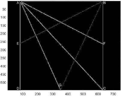
Figure 3.6 shows an image with diagonal edges of different slopes all located inside a square ABCD, where the points E, F and G are in the middle of the lines AD, BC and CD respectively. So edge BD has slope 𝑘 = 1, edge AC has slope 𝑘 = −1, edge BE has slope 𝑘 = 1/2, edge AF has slope 𝑘 = −1/2, edge BG has slope 𝑘 = 2, and finally, edge AG has slope 𝑘 = −2.
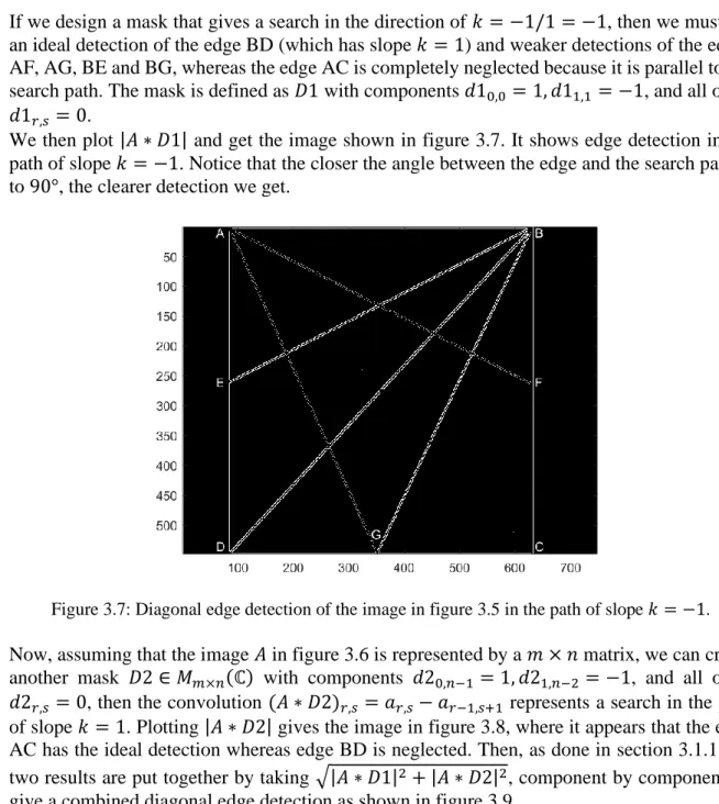
18 If we design a mask that gives a search in the direction of 𝑘 = −1/1 = −1, then we must get an ideal detection of the edge BD (which has slope 𝑘 = 1) and weaker detections of the edges AF, AG, BE and BG, whereas the edge AC is completely neglected because it is parallel to the search path. The mask is defined as 𝐷1 with components 𝑑10,0 = 1, 𝑑11,1 = −1, and all other 𝑑1𝑟,𝑠 = 0.
We then plot |𝐴 ∗ 𝐷1| and get the image shown in figure 3.7. It shows edge detection in the path of slope 𝑘 = −1. Notice that the closer the angle between the edge and the search path is to 90°, the clearer detection we get.
Figure 3.7: Diagonal edge detection of the image in figure 3.5 in the path of slope 𝑘 = −1. Now, assuming that the image 𝐴 in figure 3.6 is represented by a 𝑚 × 𝑛 matrix, we can create another mask 𝐷2 ∈ 𝑀𝑚×𝑛(ℂ) with components 𝑑20,𝑛−1 = 1, 𝑑21,𝑛−2 = −1, and all other 𝑑2𝑟,𝑠 = 0, then the convolution (𝐴 ∗ 𝐷2)𝑟,𝑠 = 𝑎𝑟,𝑠− 𝑎𝑟−1,𝑠+1 represents a search in the path of slope 𝑘 = 1. Plotting |𝐴 ∗ 𝐷2| gives the image in figure 3.8, where it appears that the edge AC has the ideal detection whereas edge BD is neglected. Then, as done in section 3.1.1, the two results are put together by taking √|𝐴 ∗ 𝐷1|2 + |𝐴 ∗ 𝐷2|2, component by component, to give a combined diagonal edge detection as shown in figure 3.9.
19 Figure 3.8: Diagonal edge detection of the image in figure 3.5 in the path of slope 𝑘 = 1.
Figure 3.9: Combined diagonal edge detection obtained by 𝐷1 and 𝐷2.
If we instead want to target the edge BG which has slope 𝑘 = 2, we design a mask that gives a search in the path of slope 𝑘 = −1/2. The mask may be defined as 𝐷3: 𝑑30,0= 1,
𝑑31,2 = −1 and all other 𝑑3𝑟,𝑠 = 0. The result is shown in figure 3.10, where we can see that the edge AF parallel to the search path is neglected.
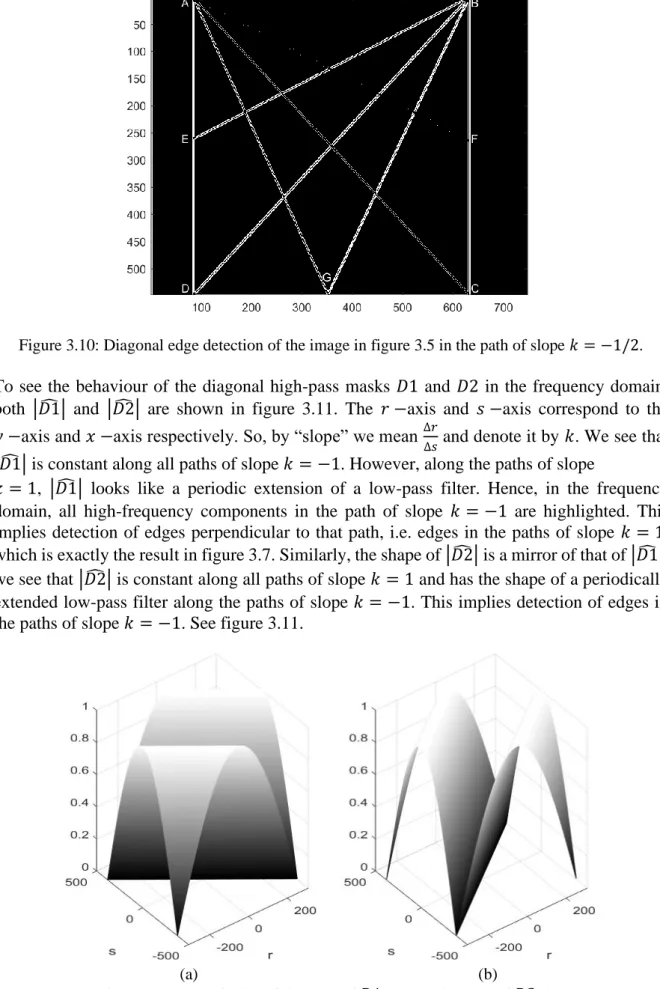
20 Figure 3.10: Diagonal edge detection of the image in figure 3.5 in the path of slope 𝑘 = −1/2. To see the behaviour of the diagonal high-pass masks 𝐷1 and 𝐷2 in the frequency domain, both |𝐷1̂ | and |𝐷2̂ | are shown in figure 3.11. The 𝑟 −axis and 𝑠 −axis correspond to the 𝑦 −axis and 𝑥 −axis respectively. So, by “slope” we mean ∆𝑟
∆𝑠 and denote it by 𝑘. We see that |𝐷1̂ | is constant along all paths of slope 𝑘 = −1. However, along the paths of slope
𝑘 = 1, |𝐷1̂ | looks like a periodic extension of a low-pass filter. Hence, in the frequency domain, all high-frequency components in the path of slope 𝑘 = −1 are highlighted. This implies detection of edges perpendicular to that path, i.e. edges in the paths of slope 𝑘 = 1, which is exactly the result in figure 3.7. Similarly, the shape of |𝐷2̂ | is a mirror of that of |𝐷1̂ |, we see that |𝐷2̂ | is constant along all paths of slope 𝑘 = 1 and has the shape of a periodically extended low-pass filter along the paths of slope 𝑘 = −1. This implies detection of edges in the paths of slope 𝑘 = −1. See figure 3.11.
(a) (b)
21 3.1.3 Technical issues with diagonal edges
Note: The discussion in this section is taken only for linear edges with positive slopes. For
negative slopes, the arguments are identical but in reverse direction. Recall, from section 2.4.2, that an edge with positive slope 𝑘 =𝑎
𝑏∈ ℚ is detected using a mask 𝐷 ∈ 𝑀𝑚×𝑛(ℂ) with components 𝑑0,0 = 1, 𝑑𝑏 ,𝑎= −1 and all other 𝑑𝑟,𝑠 = 0. The result of convolving the image matrix 𝐴 with 𝐷 is, by equation (2.7), (𝐴 ∗ 𝐷)𝑟,𝑠 = 𝑎𝑟,𝑠− 𝑎𝑟−𝑏,𝑠−𝑎. The distance between pixels 𝑎𝑟,𝑠 and 𝑎𝑟−𝑏,𝑠−𝑎 is, by the Pythagorean theorem, exactly √𝑎2+ 𝑏2. So in the case when 𝑘 = 1 (recall figure 3.7), the convolution reads (𝐴 ∗ 𝐷)
𝑟,𝑠 = 𝑎𝑟,𝑠− 𝑎𝑟−1,𝑠−1 and the distance between 𝑎𝑟,𝑠 and 𝑎𝑟−1,𝑠−1 is √12+ 12 = √2. While in the case where 𝑘 = 2 =2
1 (recall figure 3.10), the convolution reads (𝐴 ∗ 𝐷)𝑟,𝑠 = 𝑎𝑟,𝑠− 𝑎𝑟−1,𝑠−2 and the distance between 𝑎𝑟,𝑠 and 𝑎𝑟−1,𝑠−2 is √12 + 22 = √5. This does not seem to be an issue for these two cases since results in figures 3.7 and 3.10 look good.
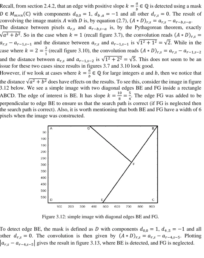
However, if we look at cases where 𝑘 =𝑎
𝑏∈ ℚ for large integers 𝑎 and 𝑏, then we notice that the distance √𝑎2+ 𝑏2 does have effects on the results. To see this, consider the image in figure 3.12 below. We see a simple image with two diagonal edges BE and FG inside a rectangle ABCD. The edge of interest is BE. It has slope 𝑘 =10
8 = 5
4. The edge FG was added to be perpendicular to edge BE to ensure us that the search path is correct (if FG is neglected then the search path is correct). Also, it is worth mentioning that both BE and FG have a width of 6 pixels when the image was constructed.
Figure 3.12: simple image with diagonal edges BE and FG.
To detect edge BE, the mask is defined as 𝐷 with components 𝑑0,0 = 1, 𝑑4 ,5 = −1 and all other 𝑑𝑟,𝑠 = 0. The convolution is then given by (𝐴 ∗ 𝐷)𝑟,𝑠 = 𝑎𝑟,𝑠− 𝑎𝑟−4,𝑠−5. Plotting |𝑎𝑟,𝑠− 𝑎𝑟−4,𝑠−5| gives the result in figure 3.13, where BE is detected, and FG is neglected.
22 Figure 3.13: Detection of edge BE, with slope 𝑘 =10
8 = 5
4, using 𝑎 = 5, and 𝑏 = 4.
However, a naive implementation of the mask 𝐷 may be based on 𝑎 = 10, and 𝑏 = 8 (since 𝑘 =10
8 = 5
4 ), so that the mask has components 𝑑0,0 = 1, 𝑑8 ,10= −1 and all other 𝑑𝑟,𝑠 = 0. Convolving this mask with the original image 𝐴 gives (𝐴 ∗ 𝐷)𝑟,𝑠 = 𝑎𝑟,𝑠− 𝑎𝑟−8,𝑠−10. Plotting |𝑎𝑟,𝑠− 𝑎𝑟−8,𝑠−10| gives the result shown in figure 3.14. Which looks different than the result in figure 3.13 even though the slope is the same in both cases. The edge FG is neglected in figure 3.14 which means correct search path, but edge BG looks thicker than its correspondent in figure 3.13, and it also looks like there are two edges BE instead of one in figure 3.14. What causes this is that the distance between the pixels 𝑎𝑟,𝑠 and 𝑎𝑟−8,𝑠−10 is √102+ 82 ≈ 12.80 while, using 𝑎 = 5, and 𝑏 = 4, the distance is √52+ 42 ≈ 6.40. So, in the case of (𝐴 ∗ 𝐷)𝑟,𝑠 = 𝑎𝑟,𝑠− 𝑎𝑟−8,𝑠−10, the distance between 𝑎𝑟,𝑠 and 𝑎𝑟−8,𝑠−10 is greater than the width of the edge itself resulting in a comparison (subtraction) between 𝑎𝑟,𝑠 to the right of the edge and 𝑎𝑟−8,𝑠−10 to the left of the edge. If 𝑎𝑟,𝑠 is just to the right of the edge BE, then 𝑎𝑟,𝑠 represents a white pixel, see figure 3.12, and 𝑎𝑟−8,𝑠−10, on the other side of the edge BE, is also white, so, we get |𝑎𝑟,𝑠− 𝑎𝑟−8,𝑠−10| = 0 = "𝑏𝑙𝑎𝑐𝑘". This explains the black line between the two white lines BE in figure 3.14. The greater √𝑎2+ 𝑏2 is, the wider the black line becomes. This black line also exists in figure 3.13, where we used 𝑎 = 5, and 𝑏 = 4, but it is so thin that it is almost not visible.
As the convolution (𝐴 ∗ 𝐷)𝑟,𝑠= 𝑎𝑟,𝑠− 𝑎𝑟−8,𝑠−10 moves to the right, i.e. as 𝑠 increases, the pixel 𝑎𝑟−8,𝑠−10 will, at some point, be at the edge BE (black) while 𝑎𝑟,𝑠 is further to the right outside of the edge (white), so |𝑎𝑟,𝑠− 𝑎𝑟−8,𝑠−10| will have a large value. This explains the second white line parallel to BE in figure 3.14.
Also, for 𝑟 and 𝑠 where 𝑟 < 8 and 𝑠 < 10, the convolution (𝐴 ∗ 𝐷)𝑟,𝑠 = 𝑎𝑟,𝑠− 𝑎𝑟−8,𝑠−10 becomes just 𝑎𝑟,𝑠. This is because 𝑎𝑟−8,𝑠−10 is outside of the image. For digital images, zero extension is used, which means that 𝑎𝑟−8,𝑠−10 = 0 and the convolution becomes (𝐴 ∗ 𝐷)𝑟,𝑠 = 𝑎𝑟,𝑠− 𝑎𝑟−8,𝑠−10= 𝑎𝑟,𝑠− 0 = 𝑎𝑟,𝑠. This explains why there are thick white margins in figure 3.14 along the upper limit AB and the left-most limit AD. The values there are just copies of their correspondents in the original image 𝐴 in figure 3.12, i.e. just 𝑎𝑟,𝑠 ∈ 𝐴. The white margin along AB has width b (in this case 8) and the white margin along AD has width a (in this case 10). The same issue exists in figure 3.13, but a and b are small there that it is barely a problem.
23 Figure 3.14: Detection of edge BE, with slope 𝑘 =10
8 = 5
4, using 𝑎 = 10, and 𝑏 = 8. To avoid these issues, it is recommended to start by simplifying the fraction 𝑘 =𝑎
𝑏, so that 𝑎 and 𝑏 are as small as possible. But, if the slope was 𝑘 =𝑎
𝑏∈ ℚ where a and b are coprime, then this issue is avoided either by approximating 𝑘 using a number 𝑘̂ = 𝑎̂
𝑏̂∈ ℚ, such that 𝑘̂ ≈ 𝑎 𝑏 as discussed in section 2.4.2, or by simply rotating the image so that the edge becomes vertical (or horizontal). A linear edge with slope 𝑘 =𝑎
𝑏∈ ℚ makes an angle of φ = tan −1 𝑎
𝑏 to the horizontal axis. To make the edge vertical, the image should be rotated by an angle of 90° − φ. Then the edge is detected using the mask 𝑉 introduced in section 2.4.1 for vertical edges.
24 3.2 Non-linear edges
Non-linear edges are edges with slopes that depend on the spatial variables (𝑥, 𝑦). This includes all edges with curved shapes. When dealing with such edges it’s convenient to stop looking for ideal solutions and rather start looking for efficiency. This is because non-linear edges are, unlike linear edges, often not possible to model mathematically and hence it’s difficult (and pointless) to look for optimal edge detections. The image in figure 2.3 (a) of section 2.5 has edges of different forms including non-linear edges. These edges can be detected by using the masks 𝐻 and 𝑉 introduced in section 2.4.1 for horizontal and vertical edges respectively. Applying these masks and combining the results using √|𝐴 ∗ 𝐻|2+ |𝐴 ∗ 𝑉|2 yield the image shown in figure 3.15. It is clear that the edge detection is rather efficient since it shows the features of the original image.
(a) (b)
Figure 3.15: Original sampled image (a) and its edges (b).
Another way to detect nonlinear edges is to use a two-dimensional high-pass mask defined in the frequency domain. Let the two-dimensional DFT of the original image in figure 2.3 (a) be denoted by 𝐴̂. Then we can assume that the five-times denoised image in figure 2.4 (b) is obtained by taking 𝐴̂ ∙ 𝐿̂, for a low-pass mask 𝐿̂. The edges of the original image are then obtained by taking 𝐴̂ ∙ 𝐻̂, for a high-pass mask 𝐻̂. Now, since 𝐴̂ = 𝐴̂ ∙ 1, it follows from remark 2.1 that 𝐴̂ = 𝐴̂ ∙ 1 = 𝐴̂ ∙ (𝐿̂ + 𝐻̂), which implies
𝐴̂ ∙ 𝐻̂ = 𝐴̂ ∙ (1 − 𝐿̂) = 𝐴̂ − 𝐴̂ ∙ 𝐿̂ 3.1
By theorem 1.1 and equation (1.11), taking the inverse Fourier transform on both sides yields
(𝐴 ∗ 𝐻) = 𝐴 − (𝐴 ∗ 𝐿) 3.2
Plotting |𝐴 ∗ 𝐻| = |𝐴 − (𝐴 ∗ 𝐿)| gives the result in figure 3.16 which shows the edges of 𝐴. This approach looks efficient and we could’ve applied it to the linear edges in the previous section, but the results would’ve not been ideal for the targeted edges. This is because the masks here are defined in the frequency domain unlike the masks in the previous section that were defined in the spatial domain to give search for edges in certain directions.
25 Figure 3.16: Edges of the original image in figure 3.15 (a), obtained by eq. 3.2.
3.3 Dealing with noise
Noise causes problems in edge detection because filters that detect edges are high-pass filters, thus they are sensitive to all high-frequency components in the image including noise. To see this, let’s recall the two images in figure 2.3, they are shown in figure 3.17 below.
Now, if we detect edges of both images in figure 3.17, we get the result shown in figure 3.18. It is clear that the edge detection of the noisy image is, due to noise, unreliable and doesn’t show the important features of the image. Suppose we are given only the noisy image and want to detect its edges, then we must first try to get rid of the noise before detecting the edges. Yet cautiousness is crucial when using a pass filter to denoise the image, this is because low-pass filters cut off high-frequency components and might harm the edges.
(a) (b)
26 In section 2.5, we used the nine-averaging mask to denoise the noisy image, the result of applying this mask once and five times are shown, again, in figure 3.19. We detect the edges in these denoised images (using masks 𝐻 and 𝑉) and the results are shown in figure 3.20. Notice that the edges in figure 3.20 (a) are sharper than those in (b) of the same figure, this is because they are less effected by the low-pass filter and hence the high-frequency components from the original image are better preserved. However, the noise obscures significant parts of the edges in figure 3.20 (a). On the other hand, the edges in figure 3.20 (b) are clearer and less disrupted by noise, but they themselves are smoother than those in image (a) of the same figure, which is expected after applying the low-pass filter five times to the noisy image. In any case, comparing the edges in figure 3.20 to the edges of the original image in figure 3.18 (a), one can argue that the result in figure 3.20 (b) is better than that in figure 3.20 (a) since it shows most significant edges with almost no disruption made by noise.
(a) (b)
Figure 3.18: (a): Edges of the original image. (b): Edges of the noisy image.
(a) (b)
27
(a) (b)
28
4 Discussion and conclusions
Edge detection is a vast subject. The purpose of this subject is to improve computer/machine vision to process images. So, for such a technical subject one should expect difficulties in finding optimal results for complicated problems. Maybe only for very simple cases that one might get optimal results. It has been seen in this work that it is possible to get ideal edge detection for linear edges using the gradient approach. But this ideality occurs at the expense of edges that are parallel (or close to parallel) to the search path. This is an advantage if one wants to highlight only linear edges of a certain kind. But one should be careful when constructing the masks not to pick a and b so that √𝑎2 + 𝑏2 is “too large”. One should simplify the fraction 𝑎
𝑏 to lowest terms. Moreover, things get even better if one finds a and b such that √𝑎2+ 𝑏2 is less than the width of the edge. This is to avoid getting that black line between two edges, as shown in figure 3.14.
The case for non-linear edges is different. This is another example of how hard it is to find perfect solution for complicated real-world problems. Yet, the results were satisfying both for linear and non-linear edges, since the results did show the important features of the images, as shown in figure 3.15 (b). There is no way we can design a mask which, based on the gradient approach, gives an ideal edge detection of non-linear edges. This is because ideal detection, as we’ve seen, is achieved by searching in the direction perpendicular to that of the edge. So, to get an ideal detection of a circular edge, say, that would mean searching perpendicularly along the edge that changes slope. This requires a mask capable of targeting all directions, which is not available. But even if such a mask was available, applying it will necessarily result in ideal detection of all edges, which is a disadvantage when we are not interested in all edges. Hence, it is more practical to decompose the process, so that we detect one kind of edges at a time, and thereafter put the results together as done in chapter 3.
In section 3.2 we presented a method for detecting edges which is not based on the gradient, recall equation (3.2). That method is rather based on frequency response in the frequency domain. The reason for presenting this method was to compare the gradient approach to another approach. Of course, there is plenty of other approaches to detect edges, for example, the Laplacian method5 and wavelets. Wavelets (in two dimensions) have the property of space-frequency localization6, so they also can be used for directional edge detection7. This is because the wavelet transforms capture image details in both spatial domain and frequency domain. It has also been shown how noise has a negative impact on edges. Which is due to the fact that both noise and edges are high-frequency components. So, the high-pass filters used to detect edges also detect and highlight noise. To handle this problem, low-pass filters were used to remove the noise. But, since low-pass filters only preserve low-frequency components, they also harm the edges the more they get applied to the image. This means that one should trade between noise removal and edge preservation until the results look satisfactory, as in figure 3.20.
29
5 Suggestions for future work
In this work the focus was on the gradient method. Since edge detection is a broad subject with different approaches, it might be a good idea in the future to compare the gradient method to another method. In this work, the results obtained by the gradient method for non-linear edges were compared to results obtained by a frequency response-based method. But this comparison was in a small margin with not much detail, not no mention that the method itself is not direction-based. So, it could be wise in the future to compare the results of directional edge detection obtained by the gradient method to results obtained by another directional method. For example, the wavelet transform, as reference [7] illustrates.
Another suggestion (this might sound out of the context of this essay) is to consider other features in images than edges. One such feature could be extreme values. In this work we’ve considered edges, that is, when ‖∇𝑓‖ is large. But, what about considering ‖∇𝑓‖ = 0? This corresponds to “peaks” and “valleys” in the image intensity. For example, if the 2D image is a set of level curves of the 3D Himmelblau8 function, then there may be a way to locate and classify the extreme values of the function from the 2D image, that is, the solver has no idea of the behaviour of the function but still can find its local optima through the colour distribution on the 2D level curves. This may include working with first derivatives (gradient) to locate the extreme values, and second derivatives (hessian) to classify the extreme values, all taken in terms of the intensity in the image showing the level curves and not in terms of the function values. But this is a story for another day …
30
6 Appendices
This chapter contains the Matlab code that was used to produce the results obtained in this work.
6.1 Code for section 2.5
close all clear; clc
% Read image
X=imread('Vivaldi.jpg'); [r,s]=size(X); L=255; map=([(0:L)/L; (0:L)/L;(0:L)/L]'); % Add noise J = imnoise(X,'gaussian',.2,0.1); figure subplot(1,2,1) colormap(map); imshow(X); subplot(1,2,2) colormap(map); imshow(J);
% Define nine-averaging mask
F=zeros(r,s); F(r/2:r/2+2,s/2:s/2+2)=1/9;
% Denoise five times and plot
Y1=conv2(F,J,'same'); Y2=conv2(F,Y1,'same'); Y3=conv2(F,Y2,'same'); Y4=conv2(F,Y3,'same'); Y5=conv2(F,Y4,'same'); figure subplot(1,2,1)
colormap(map); image(abs(Y1));set(gca,'XTick',[], 'YTick', []) subplot(1,2,2)
colormap(map); image(abs(Y5));set(gca,'XTick',[], 'YTick', [])
% Plot DFT of the nine-averaging mask
Fw=10*abs(fft2(F));
Fw=Fw(r/2-150:r/2+150,s/2-120:s/2+120);
figure;colormap([0 0 0]); mesh(-120:120,-150:150,Fw); xlabel('k'); ylabel('l'); grid on
31 6.2 Code for section 3.1.1
close all clear; clc % Read image A=imread('myImage.png'); X=A(:,:,1); [r,s]=size(X); image(X) colormap(gray) % Horizontal edges H=zeros(size(X)); H(1,1)=1; H(2,1)=-1; Ch=conv2(X,H); figure imagesc(abs(Ch(1:r,1:s))); colormap(flipud(gray)) % Vertical edges V=zeros(size(X)); V(1,1)=1; V(1,2)=-1; Cv=conv2(X,V); figure imagesc(abs(Cv(1:r,1:s))); colormap(flipud(gray)) % Combine C=abs(abs(Ch(1:r,1:s))+abs(Cv(1:r,1:s))); figure imagesc(C); colormap(flipud(gray))
% Obtain and plot the DFTs of H and V
Hw=abs(fft2(H)); Vw=abs(fft2(V)); figure
subplot(1,2,1)
colormap(gray); mesh(-s/2:s/2-1,-r/2:r/2-1,Hw); xlabel('r'); ylabel('s'); title('|DFT(H)|'); grid on subplot(1,2,2)
colormap(gray); mesh(-s/2:s/2-1,-r/2:r/2-1,Vw); xlabel('r'); ylabel('s'); title('|DFT(V)|'); grid on
32 6.3 Code for section 3.1.2
close all clear; clc
% Read image and plot
A=imread('diagonalEdges.png'); X=A(:,:,1); [r,s]=size(X); image(X);
colormap(gray)
title('Image with diagonal edges'); text(60,10,'A','linewidth', 5); text(635,10,'B','linewidth', 5); text(635,535,'C','linewidth', 5); text(60,535,'D','linewidth', 5); text(60,260,'E','linewidth', 5); text(635,260,'F','linewidth', 5); text(340,515,'G','linewidth', 5);
% Detect diagonal edges of slope k=1, so the search path has slope k=-1
D1=zeros(size(X)); D1(1,1)=1; D1(2,2)=-1; Cd1=conv2(X,D1);
figure
imagesc(abs(Cd1(1:r,1:s)));
title('Diagonal edge detection, k=1'); colormap(gray)
text(60,10,'A','linewidth', 5,'color','w'); text(635,10,'B','linewidth', 5,'color','w'); text(635,535,'C','linewidth', 5,'color','w'); text(60,535,'D','linewidth', 5,'color','w'); text(60,260,'E','linewidth', 5,'color','w'); text(635,260,'F','linewidth', 5,'color','w'); text(340,515,'G','linewidth', 5,'color','w');
% Detect diagonal edges of slope k=-1, so the search path has slope k=1
D2=zeros(size(X));
D2(1,end)=1; D2(2,end-1)=-1; Cd2=conv2(X,D2);
figure
imagesc(abs(Cd2(1:r,end-s:end)));
title('Diagonal Edge detection, k=-1'); colormap(gray)
text(60,10,'A','linewidth', 5,'color','w'); text(635,10,'B','linewidth', 5,'color','w'); text(635,535,'C','linewidth', 5,'color','w'); text(60,535,'D','linewidth', 5,'color','w'); text(60,260,'E','linewidth', 5,'color','w'); text(635,260,'F','linewidth', 5,'color','w'); text(340,515,'G','linewidth', 5,'color','w');
% Combine and plot
D=abs(abs(Cd1(1:r,1:s))+abs(Cd2(1:r,end-s:end-1))); figure
imagesc(D);
title('Combined diagonal edge detection'); colormap(gray);
33
text(60,10,'A','linewidth', 5,'color','w'); text(635,10,'B','linewidth', 5,'color','w'); text(635,535,'C','linewidth', 5,'color','w'); text(60,535,'D','linewidth', 5,'color','w'); text(60,260,'E','linewidth', 5,'color','w'); text(635,260,'F','linewidth', 5,'color','w'); text(340,515,'G','linewidth', 5,'color','w');
% Detect diagonal edges of slope k=2, so the search path has slope
% k=-1/2 D3=zeros(size(X)); D3(1,1)=1; D3(2,3)=-1; Cd3=conv2(X,D3); figure imagesc(abs(Cd3(1:r,1:s)));
title('Diagonal edge detection, k=2'); colormap(gray)
text(60,10,'A','linewidth', 5,'color','w'); text(635,10,'B','linewidth', 5,'color','w'); text(635,535,'C','linewidth', 5,'color','w'); text(60,535,'D','linewidth', 5,'color','w'); text(60,260,'E','linewidth', 5,'color','w'); text(635,260,'F','linewidth', 5,'color','w'); text(340,515,'G','linewidth', 5,'color','w');
% Obtain DFTs of D1 and D2 and plot
D1w=abs(fft2(D1))/2; D2w=abs(fft2(D2))/2; figure subplot(1,2,1) colormap(gray); mesh(-s/2:s/2-1,-r/2:r/2-1,D1w); title('|DFT(D1)|');
xlabel('r'); ylabel('s'); grid on subplot(1,2,2)
colormap(gray); mesh(-s/2:s/2-1,-r/2:r/2-1,D2w); title('|DFT(D2)|');
34 6.4 Code for section 3.1.3
close all clear; clc
% Read image and plot
A=imread('grid7.png'); X=A(:,:,1); [r,s]=size(X); image(X);
colormap(gray)
title('Image with diagonal edges BE and FG') text(20,20,'A','linewidth', 5);
text(900,20,'B','linewidth', 5); text(900,570,'C','linewidth', 5); text(20,570,'D','linewidth', 5); text(460,570,'E','linewidth', 5); text(735,295,'F','linewidth', 5); text(340,20,'G','linewidth', 5);
% Construct mask D1 using a=5 and b=4
D1=zeros(size(X)); D1(1,1)=1; D1(4,5)=-1; Cd1=conv2(X,D1);
figure
image(abs(Cd1(1:r,1:s))); colormap(gray)
title('Detection of edge BE using a=5 and b=4') text(20,20,'A','linewidth', 5,'color','w'); text(900,20,'B','linewidth', 5,'color','w'); text(900,570,'C','linewidth', 5,'color','w'); text(20,570,'D','linewidth', 5,'color','w'); text(460,570,'E','linewidth', 5,'color','w'); text(735,295,'F','linewidth', 5,'color','w'); text(340,20,'G','linewidth', 5,'color','w');
% Construct mask D1 using a=10 and b=8
D2=zeros(size(X)); D2(1,1)=1; D2(8,10)=-1; Cd2=conv2(X,D2);
figure
image(abs(Cd2(1:r,1:s))); colormap(gray)
title('Detection of edge BE using a=10 and b=8') text(20,20,'A','linewidth', 5,'color','w'); text(900,20,'B','linewidth', 5,'color','w'); text(900,570,'C','linewidth', 5,'color','w'); text(20,570,'D','linewidth', 5,'color','w'); text(460,570,'E','linewidth', 5,'color','w'); text(735,295,'F','linewidth', 5,'color','w'); text(340,20,'G','linewidth', 5,'color','w');
35 6.5 Code for section 3.2
close all clear; clc
% Read image and detect edges using H and V
X=imread('Vivaldi.jpg'); [r,s]=size(X); L=255; map=([(0:L)/L; (0:L)/L;(0:L)/L]'); % Horizontal Edges H=zeros(size(X)); H(1,1)=1; H(2,1)=-1; Ch=conv2(X,H); % Vertical Edges V=zeros(size(X)); V(1,1)=1; V(1,2)=-1; Cv=conv2(X,V); % Combine C=abs(abs(Ch(1:r,1:s))+abs(Cv(1:r,1:s))); figure subplot(1,2,1) colormap(map);
image(abs(X)); title('Original image'); set(gca,'XTick',[], 'YTick', [])
subplot(1,2,2); colormap(map);
image(abs(C)); title('Edges by gradient method'); set(gca,'XTick',[], 'YTick', [])
% Define nine-averaging mask and denoise 5 times
F=zeros(r,s); F(r/2:r/2+2,s/2:s/2+2)=1/9; Y1=conv2(X,F,'same'); Y2=conv2(Y1,F,'same'); Y3=conv2(Y2,F,'same'); Y4=conv2(Y3,F,'same'); Y5=conv2(Y4,F,'same');
% Obtain edges by subtracting denoised image from original image
S=double(X)-Y5; figure
36 6.6 Code of section 3.3 close all clear; clc
% Read image and detect edges
X=imread('Vivaldi.jpg'); [r,s]=size(X); L=255; map=([(0:L)/L; (0:L)/L;(0:L)/L]'); H=zeros(size(X)); H(1,1)=1; H(2,1)=-1; Ch=conv2(X,H); V=zeros(size(X)); V(1,1)=1; V(1,2)=-1; Cv=conv2(X,V); C=abs(abs(Ch(1:r,1:s))+abs(Cv(1:r,1:s)));
% Add noise and detect edges
J = imnoise(X,'gaussian',.2,0.1); figure
subplot(1,2,1)
colormap(map); imshow(X); title('Original image') subplot(1,2,2)
colormap(map); imshow(J); title('Noisy image') H2=zeros(size(J)); H2(1,1)=1; H2(2,1)=-1; Ch2=conv2(J,H2); V2=zeros(size(X)); V2(1,1)=1; V2(1,2)=-1; Cv2=conv2(J,V2); C2=abs(abs(Ch2(1:r,1:s))+abs(Cv2(1:r,1:s)));
% Plot edges of original and noisy image
figure
subplot(1,2,1)
colormap(map); image(abs(C));title('Edges of original image') set(gca,'XTick',[], 'YTick', [])
subplot(1,2,2)
colormap(map); image(abs(C2));title('Edges of noisy image') set(gca,'XTick',[], 'YTick', [])
% Denoise and detect edges
F=zeros(r,s); F(r/2:r/2+2,s/2:s/2+2)=1/9; % nine-averaging mask
Y1=conv2(F,J,'same'); Y2=conv2(F,Y1,'same'); Y3=conv2(F,Y2,'same'); Y4=conv2(F,Y3,'same'); Y5=conv2(F,Y4,'same');
37
% Plot noisy image filtered once and five times
figure
subplot(1,2,1)
colormap(map); image(abs(Y1)); title('Noisy image denoised once'); set(gca,'XTick',[], 'YTick', [])
subplot(1,2,2);colormap(map);image(abs(Y5)); title('Noisy image denoised five times'); set(gca,'XTick',[], 'YTick', [])
% Detect edges of noisy image filtered once and five times
H3=zeros(size(Y1)); H3(1,1)=1; H3(2,1)=-1; Ch3=conv2(Y1,H3); V3=zeros(size(Y1)); V3(1,1)=1; V3(1,2)=-1; Cv3=conv2(Y1,V3); C3=abs(abs(Ch3(1:r,1:s))+abs(Cv3(1:r,1:s))); H4=zeros(size(Y5)); H4(1,1)=1; H4(2,1)=-1; Ch4=conv2(Y5,H4); V4=zeros(size(Y5)); V4(1,1)=1; V4(1,2)=-1; Cv4=conv2(Y5,V4); C4=abs(abs(Ch4(1:r,1:s))+abs(Cv4(1:r,1:s))); figure subplot(1,2,1) colormap(map); image(abs(C3));
title('Edges of the noisy image denoised once'); set(gca,'XTick',[], 'YTick', [])
subplot(1,2,2)
colormap(map); image(abs(C4));
title('Edges of the noisy image denoised five times'); set(gca,'XTick',[], 'YTick', [])
38
References
1. based on a proof of the one-dimensional case in Broughton & Bryan - Discrete Fourier Analysis and Wavelets, Second edition, p. 146.
2. Broughton & Bryan - Discrete Fourier Analysis and Wavelets, Second edition, p. 154. 3. Portrait of Antonio Vivaldi, by François Morellon de La Cave.
4. Broughton & Bryan - Discrete Fourier Analysis and Wavelets, Second edition, p. 153.
5. G.T. Shrivakshan & Dr.C. Chandrasekar - A Comparison of various Edge Detection Techniques used in Image Processing.
6. B. Willmore, R. J. Prenger, M. C.-K. Wu and J. L. Gallant - The Berkeley Wavelet Transform: A Biologically Inspired Orthogonal Wavelet Transform.
7. Zhen Zhang, Siliang Ma, Hui Liu, Yuexin Gong - An edge detection approach based on directional wavelet transform.