Using Optimized Optimization Criteria in Ensemble Member Selection
Tuve Löfström, Ulf Johansson and Henrik Boström
Abstract — Both theory and a wealth of empirical studies
have established that ensembles are more accurate than single predictive models. Unfortunately, the problem of how to maximize ensemble accuracy is, especially for classification, far from solved. This paper presents a novel technique, where genetic algorithms are used for combining several measurements into a complex criterion that is optimized separately for each dataset. The experimental results show that when using the generated combined optimization criteria to rank candidate ensembles, a higher test set accuracy for the top ranked ensemble was achieved compared to using other measures alone, e.g., estimated ensemble accuracy or the diversity measure difficulty.
I. INTRODUCTION
he overall purpose of Information Fusion (IF) is to combine data or information from several sources, in order to provide a basis for decision making. Often this is accomplished by generating a predictive model, used for predicting an unknown (often future) value of a specific variable: the target variable. If the target value is one of a predefined number of discrete (class) labels, the task is called classification.
When performing predictive classification, the primary goal is to obtain high accuracy; i.e. few misclassifications when the model is applied to novel observations. Although some techniques like Artificial Neural Networks (ANNs) are known to consistently produce accurate models, in a wide variety of domains, the consensus in the machine learning community is that the use of ensembles all but guarantees even higher accuracy.
An ensemble is a composite model, aggregating multiple base models into one predictive model. An ensemble prediction, consequently, is a function of all included base models. The main motivation for using ensembles is the fact that combining several models using averaging will eliminate uncorrelated base classifier errors; see e.g. [1]. This reasoning, however, requires the base classifiers to commit their errors on different instances – clearly there is no point in combining identical models. Informally, the key term diversity therefore means that the base classifiers commit their errors on different instances.
The key problem is to find a suitable criterion, typically based on training or validation performance, highly correlated with ensemble accuracy on novel data. Several studies have, however, shown that natural measurements like ensemble or base classifier validation accuracy, as well as numerous diversity measurements, are poor predictors for ensemble test accuracy; see e.g., [2-4].
With this in mind, the overall purpose of this paper is to investigate whether it is beneficial to combine several atomic performance measures, obtained on training data, into a complex optimization criterion.
II. METHOD
The purpose of this study was to evaluate combinations of measures that could be used to estimate ensemble accuracy on independent test data. More specifically, we investigated using altogether four measures, either separately or somehow combined.
The four measures were: ensemble accuracy (EA), base classifier accuracy (BA), and the diversity measures Kohavi-Wolpert (KW) and difficulty (DI). It should be noted that EA is the accuracy obtained by the ensemble, while BA refers to the average accuracy obtained by the base classifiers, on a specific dataset.
We denote by l(zj) the number of classifiers that correctly recognize zj. Let L be the number of base classifiers and N the number of instances. The Kohavi-Wolpert variance [5] is defined as 2 1 1 ( )( ( )) N j j j KW l z L l z NL (1)
The difficulty measure was used in [6] by Hansen and Salomon. Let X be a random variable taking values in {0/L, 1/L,…, L/L}. X is defined as the proportion of classifiers that correctly classify an instance x drawn randomly from the data set. To estimate X, all L classifiers are run on the data set. The difficulty θ is then defined as the variance of X. The reason for including only these two diversity measures is simply the fact that they have performed better in previous studies and during initial experimentation; see e.g. [2].
Ensemble Settings
Two types of base classifier were considered in this study: ANNs and decision trees (DTs). 45 base classifiers of each type were initially generated for each training set.
Three sets of ANNs, each consisting of 15 ANNs, were generated. In the first set, the ANNs did not have a hidden layer, thus resulting in weaker models. The ANNs in the second set had one hidden layer, where the number of units, h, was based on dataset characteristics, but also slightly randomized for each ANN; see (2).
2 ( )
h
rand v c
(2) Here, v is the number of input variables and c is the number of classes. rand is a random number in the interval [0, 1]. This set represents a standard setup for ANN training.In the third set, each ANN had two hidden layers, where h1 in (3) determined the number of units in the first hidden
layer and h2 in (4) determined the number of units in the
second layer. Again, v denotes the number of input variables and c the number of classes. Naturally, the purpose of using varied architectures was to produce a fairly diverse set of ANN base classifiers
1 ( ) / 2 4 ( ( ) / )
h
v c rand v c c
(3)2 ( ( ) / )
h
rand v c c c
(4) In the experiments, 4-fold cross-validation was employed. For each fold, two thirds of the available training data was used for generating the base classifiers and one third was used for validation. All ANNs were trained without early stopping validation, leading to slightly over-fitted models. In order to introduce some further implicit diversity, each ANN used only 80 % of the available features, drawn randomly. Majority voting was used to determine ensemble classifications.The random forests considered in this study consisted of 45 unpruned, where each tree was generated from a bootstrap replicate of the training set [7], and at each node in the tree generation, only a random subset of the available features was considered for partitioning the examples. The size of the subset was in this study set to the square root of the number of available features, as suggested in [8]. The set of instances used for estimating class probabilities, i.e., the estimation examples, consisted of the entire set of training instances.
Consequently, while the set of ANN base classifiers consists of three quite distinctly different subsets of base classifiers, the set of decision trees are much more homogeneous.
Experiments
The empirical study was divided into two experiments. The purpose of the first experiment was to search for combinations of measures, able to outperform atomic measures as selection criteria. Naturally, combining accuracy measures with diversity measures fits very well into the original Krogh-Vedelsby idea; i.e. the ensembles should consist of accurate models that disagree in their predictions. The purpose of the second experiment was to evaluate the found complex performance measures. In summary, in the first experiment, promising ensembles are selected from a fixed number of available ensembles, while in the second experiment, available base classifiers are freely combined into ensembles.
In the first experiment, 5000 random ensembles, where the number of base classifiers was normally distributed between 2 and 45, were used. The base classifiers were drawn at random from the 45 pre-trained models without replacement. For the actual search, multi-objective GA (MOGA) was used to optimize the combination of measures.
Each individual in the MOGA population was represented as a vector, consisting of four float values. Each value corresponds to a weight for a specific performance measure (i.e. EA, BA, KW and DI). In Experiment 1, the complex optimization criterion used for selection was the weighted sum of the four measures. For the MOGA, the two objectives (fitness functions) used were:
Maximizing correlation between the complex optimization criterion, and the ensemble accuracy on the validation set, measured on the 5000 ensembles.
Maximizing average ensemble accuracy (on the validation set) for the top 5 % ensembles, when all 5000 were ranked using the complex optimization criterion. The purpose of the first objective was to achieve a solution that could rank the 5000 ensembles as good as possible, while the purpose of the second objective was to make the solution able to pinpoint the most accurate ensembles.
When using MOGA, the result is a set of solutions, residing in the Pareto-front. IfA { ,a1,am} is a set of
alternatives (here complex optimization criteria) characterized by a set of objectives C {C1,,CM} (here
correlation and top 5% average ensemble accuracy), then the Pareto-optimal set A A contains all non-dominated
alternatives. An alternative ai is non-dominated iff there is no other alternative aj A j, i, where aj is better than ai on all criteria.
In the experiments, three specific solutions generated by the MOGA (and consequently residing in the Pareto front) were evaluated. More specifically, first the two individual solutions with best performance on each single objective were selected. These two solutions correspond to the two edges of the Pareto front, and are very similar to solutions achieved by optimizing each objective separately. The only difference to single objective search is that if there are ties, here the solution with best performance on the second objective is guaranteed to be selected, which would not be the case in single objective search. The third solution selected was the one closest to the median of all the solutions in the Pareto front along both objectives. The Euclidian distance was used to find the ensemble closest to the median. This solution was selected, with the obvious motivation that it represents one of the most correlated solutions and at the same time one of the solutions leading to high ensemble accuracy among the top ranked ensembles. For the actual evaluation of the solutions (complex optimization criteria) found, the test set accuracy of the highest ranked ensemble, from among the 5000, is reported. Naturally, when ranking the ensembles, the weighted sum of measures, as represented by the MOGA solution, is used.
In Experiment 2, GA was again used, now for searching for ensembles maximizing a complex optimization criterion. Here, the three sets of weights found in the first experiment were used, i.e., the search was standard GA looking for an ensemble maximizing the specific complex optimization criterion used. As comparison, multi-objective GA was used with objectives EA and DI - where the solution with highest ensemble accuracy was reported. In this experiment, no restriction on the size of the ensembles was enforced, except that an ensemble should consist of at least two base classifiers. The second experiment used the same two sets of base classifiers as in the first experiment.
In Experiment 2, each individual in the GA population is a bit string of length 45, where a „1‟ in any location indicates that the base classifier with the corresponding index should be included in the ensemble.
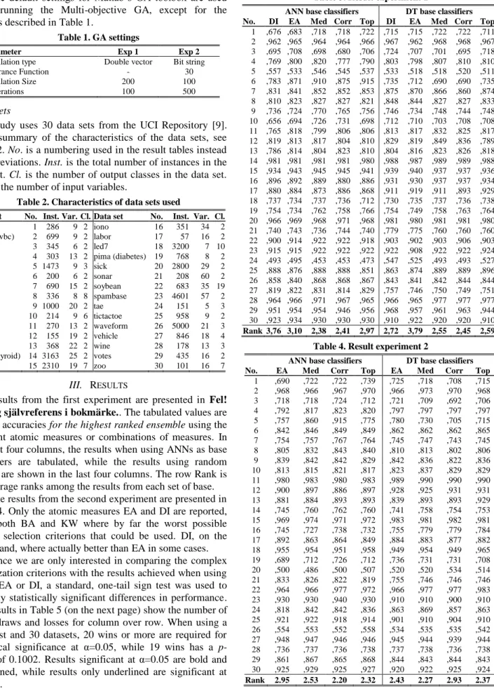
The default settings for Matlab‟s GA toolbox are used when running the Multi-objective GA, except for the settings described in Table 1.
Table 1. GA settings
Parameter Exp 1 Exp 2
Population type Double vector Bit string
Tolerance Function - 30
Population Size 200 100
Generations 100 500
Data Sets
This study uses 30 data sets from the UCI Repository [9]. For a summary of the characteristics of the data sets, see Table 2. No. is a numbering used in the result tables instead of abbreviations. Inst. is the total number of instances in the data set. Cl. is the number of output classes in the data set. Var. is the number of input variables.
Table 2. Characteristics of data sets used
Data set No. Inst. Var. Cl. Data set No. Inst. Var. Cl.
bcancer 1 286 9 2 iono 16 351 34 2 breast (wbc) 2 699 9 2 labor 17 57 16 2
bupa 3 345 6 2 led7 18 3200 7 10
cleve 4 303 13 2 pima (diabetes) 19 768 8 2
cmc 5 1473 9 3 sick 20 2800 29 2 crabs 6 200 6 2 sonar 21 208 60 2 crx 7 690 15 2 soybean 22 683 35 19 ecoli 8 336 8 8 spambase 23 4601 57 2 german 9 1000 20 2 tae 24 151 5 3 glass 10 214 9 6 tictactoe 25 958 9 2 heart 11 270 13 2 waveform 26 5000 21 3 hepati 12 155 19 2 vehicle 27 846 18 4 horse 13 368 22 2 wine 28 178 13 3 hypo (thyroid) 14 3163 25 2 votes 29 435 16 2 image 15 2310 19 7 zoo 30 101 16 7
III. RESULTS
The results from the first experiment are presented in Fel! Ogiltig självreferens i bokmärke.. The tabulated values are test set accuracies for the highest ranked ensemble using the different atomic measures or combinations of measures. In the first four columns, the results when using ANNs as base classifiers are tabulated, while the results using random forests are shown in the last four columns. The row Rank is the average ranks among the results from each set of base.
The results from the second experiment are presented in Table 4. Only the atomic measures EA and DI are reported, since both BA and KW where by far the worst possible atomic selection criterions that could be used. DI, on the other hand, where actually better than EA in some cases.
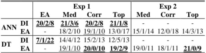
Since we are only interested in comparing the complex optimization criterions with the results achieved when using either EA or DI, a standard, one-tail sign test was used to find any statistically significant differences in performance. The results in Table 5 (on the next page) show the number of wins, draws and losses for column over row. When using a sign test and 30 datasets, 20 wins or more are required for statistical significance at α=0.05, while 19 wins has a p-value of 0.1002. Results significant at α=0.05 are bold and underlined, while results only underlined are significant at α=0.10.
Table 3. Result experiment 1
ANN base classifiers DT base classifiers No. DI EA Med Corr Top DI EA Med Corr Top
1 ,676 ,683 ,718 ,718 ,722 ,715 ,715 ,722 ,722 ,711 2 ,962 ,965 ,964 ,964 ,966 ,967 ,962 ,968 ,968 ,967 3 ,695 ,708 ,698 ,680 ,706 ,724 ,707 ,701 ,695 ,718 4 ,769 ,800 ,820 ,777 ,790 ,803 ,798 ,807 ,810 ,810 5 ,557 ,533 ,546 ,545 ,537 ,533 ,518 ,518 ,520 ,511 6 ,783 ,871 ,910 ,875 ,915 ,735 ,712 ,690 ,690 ,735 7 ,831 ,841 ,852 ,852 ,853 ,875 ,870 ,866 ,860 ,874 8 ,810 ,823 ,827 ,827 ,821 ,848 ,844 ,827 ,827 ,833 9 ,736 ,724 ,770 ,765 ,756 ,746 ,734 ,748 ,744 ,748 10 ,656 ,694 ,726 ,731 ,698 ,712 ,710 ,703 ,708 ,708 11 ,765 ,818 ,799 ,806 ,806 ,813 ,817 ,832 ,825 ,817 12 ,819 ,813 ,817 ,804 ,810 ,829 ,819 ,849 ,836 ,789 13 ,786 ,814 ,804 ,823 ,810 ,804 ,816 ,823 ,826 ,818 14 ,981 ,981 ,981 ,981 ,980 ,988 ,987 ,989 ,989 ,988 15 ,934 ,943 ,945 ,945 ,941 ,939 ,940 ,937 ,937 ,936 16 ,896 ,892 ,889 ,880 ,886 ,931 ,930 ,937 ,937 ,934 17 ,880 ,884 ,873 ,886 ,868 ,911 ,919 ,911 ,893 ,929 18 ,737 ,734 ,737 ,736 ,712 ,730 ,735 ,737 ,736 ,738 19 ,754 ,734 ,762 ,758 ,766 ,754 ,749 ,758 ,763 ,764 20 ,966 ,969 ,968 ,971 ,968 ,981 ,980 ,981 ,981 ,980 21 ,740 ,743 ,736 ,744 ,740 ,779 ,775 ,760 ,760 ,760 22 ,900 ,914 ,922 ,922 ,918 ,903 ,902 ,903 ,906 ,903 23 ,915 ,915 ,922 ,922 ,922 ,922 ,908 ,922 ,922 ,924 24 ,493 ,495 ,453 ,453 ,473 ,547 ,525 ,493 ,493 ,527 25 ,888 ,876 ,888 ,888 ,851 ,863 ,874 ,889 ,889 ,896 26 ,858 ,840 ,868 ,868 ,867 ,843 ,841 ,842 ,844 ,844 27 ,819 ,822 ,831 ,814 ,829 ,757 ,746 ,750 ,749 ,751 28 ,964 ,966 ,971 ,967 ,965 ,966 ,965 ,977 ,977 ,977 29 ,951 ,954 ,954 ,946 ,956 ,968 ,957 ,961 ,963 ,944 30 ,923 ,934 ,930 ,930 ,930 ,910 ,922 ,920 ,920 ,910 Rank 3,76 3,10 2,38 2,41 2,97 2,72 3,79 2,55 2,45 2,59
Table 4. Result experiment 2
ANN base classifiers DT base classifiers No. EA Med Corr Top EA Med Corr Top
1 ,690 ,722 ,722 ,739 ,725 ,718 ,708 ,715 2 ,968 ,966 ,967 ,970 ,966 ,973 ,970 ,968 3 ,718 ,718 ,724 ,712 ,721 ,709 ,692 ,706 4 ,792 ,817 ,823 ,820 ,797 ,797 ,797 ,797 5 ,757 ,860 ,915 ,775 ,780 ,730 ,705 ,715 6 ,842 ,846 ,849 ,849 ,862 ,862 ,862 ,865 7 ,754 ,757 ,767 ,764 ,745 ,747 ,743 ,745 8 ,805 ,832 ,843 ,840 ,810 ,813 ,802 ,806 9 ,839 ,842 ,842 ,829 ,842 ,836 ,822 ,836 10 ,813 ,815 ,821 ,817 ,823 ,837 ,829 ,829 11 ,980 ,983 ,980 ,983 ,989 ,990 ,990 ,990 12 ,900 ,897 ,886 ,897 ,928 ,925 ,931 ,931 13 ,881 ,884 ,893 ,893 ,839 ,893 ,893 ,929 14 ,745 ,760 ,762 ,760 ,741 ,758 ,754 ,753 15 ,969 ,974 ,971 ,972 ,983 ,981 ,982 ,981 16 ,745 ,727 ,738 ,732 ,755 ,779 ,779 ,784 17 ,892 ,863 ,864 ,849 ,884 ,883 ,877 ,882 18 ,955 ,954 ,951 ,958 ,949 ,954 ,949 ,965 19 ,689 ,712 ,726 ,712 ,736 ,731 ,731 ,708 20 ,500 ,486 ,500 ,507 ,520 ,520 ,534 ,514 21 ,833 ,826 ,822 ,819 ,755 ,746 ,746 ,746 22 ,964 ,966 ,977 ,972 ,966 ,977 ,977 ,983 23 ,930 ,930 ,940 ,930 ,910 ,910 ,900 ,910 24 ,818 ,842 ,842 ,836 ,863 ,869 ,857 ,863 25 ,921 ,922 ,918 ,914 ,901 ,910 ,904 ,910 26 ,554 ,553 ,552 ,558 ,534 ,535 ,535 ,542 27 ,948 ,947 ,946 ,946 ,945 ,944 ,939 ,944 28 ,736 ,737 ,736 ,738 ,737 ,738 ,736 ,738 29 ,861 ,867 ,865 ,868 ,844 ,843 ,844 ,843 30 ,925 ,929 ,925 ,927 ,920 ,922 ,925 ,924 Rank 2.95 2.53 2.20 2.32 2.43 2.27 2.93 2.37
Table 5. Wins/Draws/Losses. Exp 1 and 2
Exp 1 Exp 2
EA Med Corr Top Med Corr Top ANN DI 20/2/8 21/3/6 20/2/8 21/1/8 - - -
EA - 18/2/10 19/1/10 13/0/17 15/1/14 12/0/18 14/3/13
DT DI 7/1/22 14/4/12 15/2/13 12/5/13 - - - EA - 19/1/10 20/0/10 19/2/9 19/0/11 18/1/11 21/0/9 As can be seen in Table 5, the results achieved using the complex optimization criterions are, in most cases, clearly better than using only EA or DI as selection criterion. It is obvious that the atomic measure that is good for one set of base classifiers is not at all competitive for the other set. While DI is comparably good as selection criteria for DTs, where it is significantly better than EA, it does not work at all for ANNs, where it is significantly worse than all other selection criterions. The opposite is true for EA, which works comparably well for ANNs, but is significantly worse than all other selection criterions for DTs. In fact, only the complex optimization criterions are competitive regardless of which set of base classifiers that are used.
The results in Table 6 show wins/draws/losses comparisons between the results achieved in experiment 2 (column) over the results from experiment 1 (row).
Table 6. Wins/Draws/Losses. Exp 2 vs. Exp 1
W/D/L Exp 2
Exp 1 EA Med Corr Top ANN DI 24/0/6 25/0/5 23/0/7 26/0/4 EA 20/0/10 22/0/8 25/0/5 24/0/6 Med 17/0/13 16/0/14 19/0/11 19/1/10 Corr 14/0/16 19/0/11 21/0/9 21/0/9 Top 19/0/11 20/0/10 21/0/9 22/0/8 DT DI 13/0/17 17/0/13 15/0/15 16/0/14 EA 19/0/11 22/0/8 20/0/10 22/0/8 Med 13/0/17 15/0/15 15/0/15 19/0/11 Corr 15/0/15 16/0/14 14/0/16 19/0/11 Top 13/0/17 14/0/16 15/0/15 14/0/16 When comparing the results achieved in experiment 2 to the results from experiment 1, it is obvious that the unlimited search among all possible ensembles from the 45 base classifiers are very competitive to the approach of selecting from a smaller subset (here 5000) of solutions. This is despite the fact that these 5000 ensemble were actually the ones used for finding the optimization criteria. It is worth noting that all of the complex optimization criterions achieved in experiment 2 are significantly better than the results achieved with EA in experiment 1. They are also significantly better than using DI as selection criteria when using ANNs as base classifiers.
It is hard to single out any of the three alternative complex optimization criterions as a clear winner. If considering the two different sets of base classifiers and the two experiments as altogether four different alternative runs, the most correlated solution was very good in most cases, but it was comparably unsuccessful for DTs in experiment 1. The Top solution was successful with DTs, but failed with ANNs. The most median solution was a rather stable and always good enough choice.
IV. CONCLUSIONS
The results show clearly that using a complex optimization criterion is a very competitive choice. It is always as good as, and often better than, using any atomic measure for selection.
The results also highlight that using other measures than EA as selection criterion can be a good choice. In this study, the diversity measure DI outperformed EA as selection criterion for homogeneous base classifiers (here DTs), even though it was ensemble accuracy on the test set that was measured. However, DI did not work well for the heterogeneous set of base classifiers (here ANNs).
While different atomic measures worked well for different types of base classifiers, the complex optimization criterions worked very well for both. With this in mind, the presented approach has shown to be well worth further investigation.
Furthermore, the fact that other atomic measures (here DI) could outperform performance measures as selection criteria suggests further analysis of alternative measures, and in particular the DI measure.
ACKNOWLEDGMENT
This work was supported by the Information Fusion Research Program (University of Skövde, Sweden) in partnership with the Swedish Knowledge Foundation under grant 2003/0104 (URL: http://www.infofusion.se).
REFERENCES
[1] T.G. Dietterich, “Machine learning research: Four current directions,” AI Magazine, vol. 18, 1997, ss. 97-136.
[2] U. Johansson, T. Löfström, and L. Niklasson, “The Importance of Diversity in Neural Network Ensembles - An Empirical Investigation,” 2007, ss. 661-666. [3] L.I. Kuncheva and C.J. Whitaker, “Measures of
Diversity in Classier Ensembles and Their Relationship with the Ensemble Accuracy,” Machine Learning, vol. 51, 2003, ss. 181-207.
[4] T. Löfström, U. Johansson, and H. Boström, “The Problem with Ranking Ensembles Based on Training or Validation Performance,” Proceedings of World Congress of Computer Intelligence, 2008.
[5] R. Kohavi and D.H. Wolpert, “Bias plus variance decomposition for zero-one loss functions,” Machine Learning: Proceedings of the Thirteenth International Conference, 1996.
[6] L. Hansen and P. Salomon, “Neural Network Ensembles,” IEEE Transactions on Pattern Analysis and Machine Intelligence, vol. 12, 1990, ss. 933-1001. [7] L. Breiman, “Bagging Predictors,” Machine Learning,
vol. 24, 1996, ss. 123-140.
[8] L. Breiman, “Random Forests,” Machine Learning, vol. 45, 2001, ss. 5-32.
[9] A. Asuncion and D.J. Newman, “UCI machine learning repository,” School of Information and Computer Sciences. University of California, Irvine, California, USA, 2007.