M¨
alardalen University Press Doctoral Dissertation
No. 22
O
PTIMAL
S
TOPPING
D
OMAINS
AND
R
EWARD
F
UNCTIONS FOR
D
ISCRETE
T
IME
A
MERICAN
T
YPE
O
PTIONS
Henrik J¨
onsson
October 2005
Department of Mathematics and Physics
M¨
alardalen University
This work was funded by the Graduate School in Mathematics and Computing:
Copyright c° Henrik J¨onsson, 2005 ISSN 1651-4238
ISBN 91-85485-00-4
Contents
List of papers v
Acknowledgement vi
Abstract vii
Introduction
1 An informal introduction to the studies 1
1.1 European and American options . . . 1
1.1.1 Standard payoff functions . . . 2
1.1.2 Non-standard payoff functions . . . 3
1.2 Asset price evolution . . . 4
1.2.1 Discrete time models . . . 5
1.3 Early exercise of American type options . . . 6
1.4 Optimal stopping domains for American type options . . . 8
1.5 Description of the studies . . . 10
1.5.1 The structure of the optimal stopping domains . . . 10
1.5.2 Convergence of the reward functions . . . 12
2 American type options and optimal stopping in discrete time 13 2.1 Markovian asset price evolution . . . 13
2.2 Time inhomogeneous and non-standard payoff functions . . . 15
2.3 Optimal stopping . . . 16
2.3.1 Formulation of the problem . . . 16
2.3.2 Stopping times . . . 16
2.3.3 Backward induction, optimal stopping domains, and optimal stop-ping time . . . 17
2.4 Pricing of American options . . . 20
2.4.1 Risk-neutrality . . . 21
2.4.2 The arbitrage pricing method . . . 23
2.4.3 The optimal stopping strategy of the holder . . . 23
2.4.4 The early exercise premium representation . . . 24
2.5 Structure of the optimal stopping domains . . . 26
2.5.1 Standard American options . . . 26
2.5.2 Dividends and the optimal stopping domains . . . 29
2.5.3 Non-standard American options . . . 31
2.6 Convergence of American option values from discrete- to continuous-time models . . . 32
2.7 Main problems studied in the thesis . . . 35
2.7.1 Structural studies of the optimal stopping domains . . . 36
2.7.2 Convergence of the reward functions . . . 36
3 Summary of the papers 37 3.1 Paper A . . . 37
3.2 Paper B . . . 40
3.3 Paper C and Paper D . . . 44
3.3.1 Non-increasing payoffs (Paper C) . . . 45
3.3.2 Non-decreasing payoffs (Paper D) . . . 46
3.4 Paper E . . . 48
4 Sammanfattning p˚a svenska 51
List of papers
The present thesis contains the following five papers:
Paper A. J¨onsson, H. (2001), Monte Carlo studies of American type call options with discrete time, Theory of Stochastic Processes 7(23), 163-188. In: Proceedings of the International School on Mathematical and Statistical Applications in Economics, 2001, V¨aster˚as, Sweden.
Paper B. J¨onsson, H., Kukush, A.G., and Silvestrov, D.S. (2002), Threshold structure of optimal stopping domains for American type options, Theory of Stochastic Processes 8(24), 169-177. In: Proceedings of the Conference Dedicated to the 90th Anniver-sary of Boris Vladimirovich Gnedenko, 2002, Kyiv, Ukraine.
Paper C. J¨onsson, H., Kukush, A.G., and Silvestrov, D.S. (2004), Threshold structure of optimal stopping strategies for American type option. I, Teoriya ˘Imovirnoste˘ı ta Matematychna Statystyka 71, 82-92. (English version of the journal, published by AMS, has the title Theory of Probability and Mathematical Statistics.)
Paper D. J¨onsson, H., Kukush, A.G., and Silvestrov, D.S. (2005), Threshold structure of optimal stopping strategies for American type option. II, Teoriya ˘Imovirnoste˘ı ta Matematychna Statystyka 72, 42-53.
Paper E. J¨onsson, H. (2005), Convergence of Reward Functions in a Discrete Time Op-timal Stopping Problem: Application to American Type Options, Research Report 2005-3, Department of Mathematics and Physics, M¨alardalen University, 31 pages. Parts of this thesis have been presented at the following conferences:
1. International School on Mathematical and Statistical Applications in Economics, January 15-19, 2001, V¨aster˚as, Sweden.
2. The Conference Dedicated to the 90th Anniversary of Boris Vladimirovich Gnedenko, June 3-7, 2002, Kyiv, Ukraine.
3. 6th World Congress of the Bernoulli Society for Mathematical Statistics and
Probability, and 67th Annual Meeting of the Institute of Mathematical Statistics,
Barcelona, July 26-31, 2004.
4. International Conference on Stochastic Finance 2004, Lisbon, September 26-30, 2004. 5. Open House at Graduate School in Mathematics and Computing, and Graduate
Acknowledgement
I am very grateful to my supervisor Professor Dmitrii Silvestrov for his encouraging and inspiring supervision during my work with this doctoral thesis. Our cooperation has given me more than just deeper knowledge in mathematics and mathematical research.
I also would like to thank my assistant supervisors Professor Alexander Kukush, for his valuable comments and fruitful cooperation, and Professor Kenneth Holmstr¨om, for his support of my work.
Many thanks also to my colleagues at the Department of Mathematics and Physics, M¨alardalen University, for their support.
I thank the Graduate School in Mathematics and Computing (Forskarskolan i matem-atik och ber¨akningsvetenskap) for the financial support making it possible for me to conduct my studies.
Finally, I thank the Swedish Institute for their financial support, in the framework of the Visby programme, of my two visits to Kyiv, Ukraine, in September-October 2003 and December 2003 - January 2004.
V¨aster˚as, October 2005 Henrik J¨onsson
Abstract
In this thesis, we present studies of the discrete time optimal stopping problem corre-sponding to the early exercise of American type options in discrete time markets.
The thesis contains results presented in the five papers listed above. In the first paper, Paper A, we present an experimental study of the structure of the optimal stopping domains for various types of payoff functions, such as, piecewise linear, stepwise, quadratic and logarithmic. Also classification errors are analyzed.
In the second paper, Paper B, sufficient local conditions on non-negative, non-decreasing, convex payoff functions are given, such that the optimal stopping domains have a one-threshold structure, i.e., the optimal stopping domains are semi-infinite intervals. The underlying asset follows a time inhomogeneous geometric random walk.
In the third and fourth paper, Paper C and Paper D, we extend the results given in Paper B, assuming that the underlying asset follows a general discrete time Markov process. In these two papers, the sufficient conditions for the stopping domains to have a one-threshold structure are given for convex payoff functions that are non-increasing (corresponding to put type options) and non-decreasing (call type options) in Paper C and Paper D, respectively.
In the last paper, Paper E, we present convergence results for the reward functions for discrete time optimal stopping problems, corresponding to a family of American type options in discrete time markets, under the assumption that the transition probabilities of the underlying price processes and the payoff functions depend on a “perturbation” parameter and converge to corresponding “unperturbed” limit quantities. The underlying price processes are inhomogeneous discrete time Markov processes and the payoff functions are time inhomogeneous monotone functions.
Introduction
1
An informal introduction to the studies
The topic of the present thesis is presented in this section in an informal manner. It is supposed to be an introduction that is accessible to anyone who has none or just a little knowledge of options and higher mathematics. In Section 2 of the present thesis, we give a more formal presentation of the topic and discuss more rigorously the theory in the studies. Here the optimal stopping problem is formulated and the solution method is formalized. The summary of the results from the five papers that are included in the thesis is given in Section 3.
1.1
European and American options
An option is a contract on the financial market giving the holder the right, but not the obligation, to buy or sell an underlying asset for a pre-specified price, called the strike price. If the holder has the right to buy the underlying asset the option is called a call option, and if the holder has the right to sell it is called a put option. An option is only valid for a pre-specified time period. The last date of validity is called the expiration date. To receive this right the holder has to pay a premium, the price of the option, to the writer of the option.
When the holder decides to use the right to buy or sell the underlying asset it is said that the option is exercised. The type of exercise of the option is also pre-specified. If the option is of European type, it is only possible to exercise the option at the expiration date. If the option is of American type, the exercise of the option can be made at any moment up to and including the expiration date.
Examples of underlying assets are stocks, currencies, indices, and other financial con-tracts.
We consider only options of American type in this thesis.
For a general introduction to options see, e.g., Jarrow and Turnbull (2000) and Hull (2006). We would like also to refer to some well known books on mathematical finance: Pliska (1997), Shiryaev (1999), Karatzas and Shreve (2001), Bj¨ork (2004), F¨ollmer and Schied (2004), Shreve (2004a, 2004b), and Musiela and Rutkowski (2005).
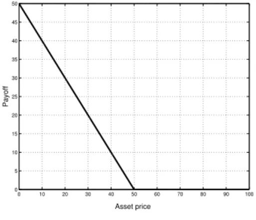
0 10 20 30 40 50 60 70 80 90 100 0 5 10 15 20 25 30 35 40 45 50 Asset price Payoff
(a) American call option.
0 10 20 30 40 50 60 70 80 90 100 0 5 10 15 20 25 30 35 40 45 50 Asset price Payoff
(b) American put option.
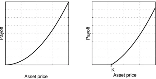
Figure 1: Standard payoff function for American call and put option, respectively, with strike price K = 50.
1.1.1 Standard payoff functions
The option’s payoff describes the value of exercising the option, and is, of course, depen-dent on the value of the underlying asset (and the strike price).
The payoff is described by the payoff function g acting from R+ to R+.
We will treat the exercise of the option as a transaction of the payoff g(s) to the holder from the writer, where s is the value of the underlying asset. That is, if the holder exercises a call option, we do not assume that he receives the underlying asset, we just assume that he receives the payoff g(s).
This is similar to assume that the holder receives the underlying asset and immediately sells the asset for the price s, without paying any fees, etc, that is, the transactions are made on a frictionless market.
Example 1. Standard American call option. At any time up to and including the expiration date T the holder has the right to exercise the option. When the option is exercised the holder pays the strike price K for the underlying asset with value s.
If s < K, the holder does not exercise the option, since he would spend K for something worth s. On the other hand, if s > K, the holder could exercise the option and receive the payoff s − K > 0. Thus, the payoff for the standard American call option is given by g(s) = [s − K]+ = max{0, s − K}. (1) Figure 1(a) shows a payoff function for a standard American call option.
Example 2. Standard American put option. At any time up to and including the expiration date T the holder has the right to exercise the option. When the option is exercised the holder receives the strike price K for the underlying asset with value s.
If s > K, the holder does not exercise the option, since he would receive K for something worth s. On the other hand, if s < K, the holder could exercise the option and receive the payoff K − s > 0. Thus, the payoff for the standard American put option is given by
g(s) = [K − s]+ = max{0, K − s}. (2) Figure 1(b) shows a payoff function for a standard American put option.
1.1.2 Non-standard payoff functions
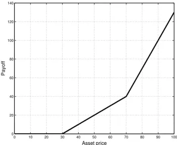
In this thesis we will consider American options with more complicated payoff functions than the standard functions (1) and (2). In particular, call options with convex, non-decreasing payoff functions, and put options with convex, non-increasing payoff functions. An example of one such type of payoff function considered is the piecewise linear function given in Figure 2. 0 10 20 30 40 50 60 70 80 90 100 0 20 40 60 80 100 120 140 Asset price Payoff
Figure 2: Piecewise linear payoff function for an American
type call option with strike prices K1 = 30 and K2 = 70,
1.2
Asset price evolution
There are two alternatives to model the financial markets, either using continuous time models or discrete time models. In the present thesis we consider discrete time models only. However, we begin with a short description of the standard model used in continuous time, the geometric Brownian motion.
In the continuous time models the market is assumed to operate continuously. The price of the underlying asset is assumed to change continuously with time and the Amer-ican option can be exercised at any moment up to and including the expiration date.
Traditionally the value of the underlying asset in the continuous market is considered to follow a diffusion process. This idea was presented 1900 by Louis Bachelier in his thesis. He proposed that the prices follows a stochastic process called Brownian motion, i.e.,
St = S0+ µt + σWt, t ≥ 0,
where S0 is the initial price, µ and σ is the drift and the volatility per time unit,
respec-tively, of the process and Wt is a standard Brownian motion (or Wiener process), i.e., a
process with independent normal increments and continuous trajectories, satisfying the following conditions W0 = 0, EWt= 0, EWt2 = t.
However, this model was later improved as it was proposed that it is the logarithm of the prices that approximately follows a Brownian motion and not the prices themselves. That is, the standard model used to describe the evolution of the asset prices in continuous time is the so called geometric Brownian motion
St= S0eµt+σWt, t ≥ 0. (3)
The characteristic of the geometric Brownian motion is that it has continuous trajec-tories and independent and log-normal distributed multiplicative increments.
There are several extensions of the geometric Brownian motion, e.g., jump-diffusion processes. We will not discuss the continuous time models in details in this thesis. How-ever, many results about American options in the literature are given for continuous time models. See for example the discussion about the pricing of American options in Section 2.4 and the optimal stopping domains in Section 2.5.
More information about the Brownian motion and its applications, e.g., in mathemat-ical finance, can be found in the books by Borodin and Salminen (2002) and Øksendal (2003).
1.2.1 Discrete time models
In this thesis we consider discrete time financial markets, i.e., markets which are assumed to operate at discrete moments. Thus, the value of the underlying asset changes at discrete moments and the American option can be exercised at discrete moments only. The discrete time models can be viewed as approximations of the continuous time models. However, the discrete time models have their own value and right of existence, in particular in connection with computer simulation methods.
Let us assume that our discrete time market operates at the moments 0, 1, 2, . . .. One commonly used discrete time model is the geometric random walk, where the value Sn of the underlying asset at moment n is given by the value Sn−1 of the process at
moment n − 1 multiplied with a nonnegative random variable Yn,
Sn = Sn−1Yn, n = 1, 2, . . . . (4)
We can choose different distributions for the random variables Yn and we can choose
whether the random variables Y1, Y2, . . . should be independent or not, and whether they
should be identically distributed or not. Note that we can write (4) as
Sn= s0 n
Y
i=1
Yi, n = 1, 2, . . . .
A very popular discrete time model is the Cox-Ross-Rubinstein-model, or the Binomial model, first proposed in Cox, Ross, and Rubinstein (1979). In this model, the value of the underlying asset can, starting from Sn−1 at moment n − 1, only assume two values at
moment n, i.e., either Yn = u or Yn = d, where u and d are non-negative constants, and
P {Yn = u} = p and P {Yn = d} = 1 − p. If we assume that 0 < d < 1 < u we have a
model where the value of the process either increases with a factor u or decreases with a factor d.
It should be noted that the parameters u, d and p depend on the length of the time step (in this case we have chosen the length to equal 1). With suitable re-scaling of time and choices of the parameters u, d and p, the Binomial model converges to the geometric Brownian motion (3) as the changes in the value of the underlying asset becomes more and more frequent, i.e., the time between two jumps tends to zero.
The Binomial model (or CRR-model) is the simplest example of a family of discrete time models called tree models. In the tree models we assume the processes to take values in a discrete phase space, that is, the random variable Yn in (4) is a discrete
random variable that can assume only a finite number of values. The tree models are powerful in the sense that they are easy to understand and implement.
Another approach is to model directly the geometric random walk such that increment between two moments has the same distribution as a continuous time model over the same time interval, for example log-normal. Thus we can create a discrete time analogy to the continuous time geometric Brownian motion in (3) by choosing Yn = eµ+σξn, where ξn is
a standard normal random variable (i.e., a normal random variable with Eξn = 0 and
Eξ2
n= 1). By this choice each Yn is a log-normal random variable and we get a geometric
random walk with log-normal increments where the value of the process at moment n is given by
Sn= S0eµn+σ Pn
i=1ξi, n = 1, 2, ..., (5)
where we assume that ξ1, ξ2, . . . are independent standard normal random variables.
We can create a continuous time process from the discrete time process by assuming that the discrete time process is constant between the moments of change, i.e., St = Sn if
n ≤ t < n + 1.
See, for example, Pliska (1997), Shiryaev (1999), Bj¨ork (2004), F¨ollmer and Schied (2004), and Musiela and Rutkowski (2005), for details about the continuous and discrete time models used in financial mathematics.
1.3
Early exercise of American type options
Assume that the option can be exercised at any of the moments 0, 1, 2, . . . , N , where N is the expiration date.
If the option is exercised at moment 0 ≤ n ≤ N , the present value of the profit is −C + e−rn
g(Sn), (6)
where C is the price of the option paid to the writer at moment 0 , r is the continuously compounded risk free interest rate per time unit, and e−rng(S
n) is the present value of
the payoff if the option is exercised at moment n.
The problem for the holder is to determine the moment which is optimal for exercising the option. Here we mean optimal in the sense that the expected present value of the profit is maximized. The decision to exercise the option at time τ should be based on the information available at that time. The future should be unknown. That is, all past prices and the present price of the underlying asset are known and should be used, but
all future prices of the underlying asset are unknown. Accordingly, only those moments satisfying this condition are admissible when we want to maximize the expected present value of the profit.
We should therefore take the expected value of the profit (6) and maximize it over all admissible times τ , 0 ≤ τ ≤ N . Since the option price C is a constant the optimal exercise strategy does not depend on it and we can maximize the expected present value of the payoff over 0 ≤ τ ≤ N ,
max
0≤τ ≤NE e
−rng(S
n). (7)
To find the optimal moment to exercise the option such that the expected profit is maximized is a typical optimal stopping problem. The optimal moment to exercise the option is called the optimal stopping time.
From the general theory of optimal stopping we know that the decision to exercise or not should be based on the present price of the underlying asset only (see e.g. Chow, Robbins, and Siegmund (1971), and Shiryaev (1978)). That is, by knowing the value of the underlying asset at time τ we can decide whether to exercise or not.
Furthermore, since the decision to exercise or not is based on the present price of the underlying asset, we can at each moment identify those asset prices such that it is optimal to stop. We can, therefore, at each moment divide the asset prices into two sets, the optimal stopping domain and the continuation domain. The optimal stopping domain, also called the early exercise region, contains all asset prices such that it is optimal to exercise. The continuation domain contains all asset prices such that it is better to wait with the exercise, i.e., to continue to hold the option.
The boundary of the optimal stopping domain is called the optimal stopping boundary or the early exercise boundary.
An example of optimal stopping domains for a discrete time optimal stopping problem where the underlying process is a geometric random walk with log-normal increments is given in Figure 3.
To determine which asset values are in the optimal stopping domain and which are in the continuation domain we use reward functions. The reward function represents, at each moment n = 0, 1, . . . , N , the value of the optimal strategy at moment n given the asset value Sn.
For any asset value Sn in the optimal stopping domain for moment n the optimal
strategy is, by definition, to stop and receive the payoff g(Sn). Accordingly, the value of
in the optimal stopping domain.
On the contrary, for any asset value Sn belonging to the continuation domain the
optimal strategy is to continue and the value of the reward function is, therefore, equal to the expected discounted value of the optimal strategy at the next moment.
Hence, for each asset value we compare the payoff if the option is exercised with the expected future profit if we continue to hold the option. Whatever value is greater defines the optimal strategy for that asset value.
The optimal moment to exercise the option, i.e., the optimal stopping time, such that the expected profit is maximized, is given by the first moment the value of the underlying asset enters the optimal stopping domain (see Chow, Robbins, and Siegmund (1971), and Shiryaev (1978)). Consequently the optimal moment to exercise is a so called first hitting time or a first passage time.
1.4
Optimal stopping domains for American type options
As described above, the optimal moment to exercise the option is equal to the first time the price of the underlying asset enters the optimal stopping domain.
Hence, for each moment 0 ≤ n ≤ N , we need to know which prices are in the optimal stopping domain and which are not. That is, we need to know the structure of the optimal stopping domains.
The structure of the optimal stopping domains and the boundary of the domains for the standard American put and call options has been studied in, e.g., Van Moerbeke (1976), Kim (1990), Jacka (1991), Carr, Jarrow, and Myneni (1992), Myneni (1992), Shiryaev (1994), and Broadie and Detemple (1999). These studies were motivated by the problem of pricing the option. Since the American option can be exercised early this feature must be included into the problem of pricing the option and, therefore, it is important to understand the structure and the properties of the optimal stopping domains and the optimal stopping boundary.
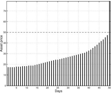
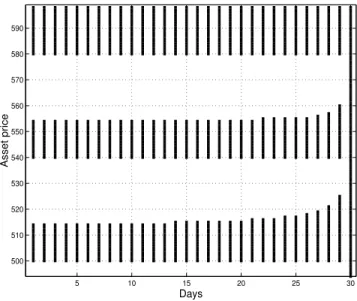
For the standard American call option in a discrete time model, where the underlying asset follows a geometric random walk with log-normal increments, the optimal stopping domains have the structure given in Figure 3.
As seen in Figure 3, the stopping domain for each moment n is a semi-infinite interval. Consequently, at each moment n, there exists a threshold value dn of the underlying asset
such that the option is exercised optimally for every asset value greater than or equal to dn. The value dn is some times called the critical value or the critical price.
5 10 15 20 25 30 35 40 45 50 0 10 20 30 40 50 60 70 80 90 Days Asset price
Figure 3: Example of the structure of the optimal stopping domains (black) for a standard American call option in a discrete time model where the option can be exercised at any moment n = 1, . . . , 50. The strike price K = 25 is marked with the dashed line. The underlying asset follows a geometric random walk with log-normal increments.
5 10 15 20 25 30 35 40 45 50 0 10 20 30 40 50 60 70 Days Asset price
Figure 4: Example of the structure of the optimal stopping domains (black) for a standard American put option in a discrete time model where the option can be exercised at any moment n = 1, . . . , 50, which is the expiration date. The strike price K = 50. The underlying asset follows a geometric random walk with log-normal increments.
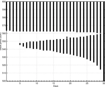
The structure of the optimal stopping domains for a standard put option in a discrete time model, where the underlying asset follows a geometric random walk with log-normal increments, is shown in Figure 4. Also for the standard American put option there exist a critical value dn for each moment n. But for the put option all values less than or equal
to dn are in the optimal stopping domain.
Due to the early exercise feature there exist in general no analytical solutions to the pricing problem of American type options. However, if the structure of the optimal stopping domains is known, different numerical procedures, such as the Monte Carlo method, can be applied to calculate the price of the option.
The knowledge of the structure of the optimal stopping domains can also be used in Monte Carlo algorithms to analyze different characteristics of the early exercise, such as, the average exercise time and the probability of early exercise.
1.5
Description of the studies
In this thesis we study the discrete time optimal stopping problem for the holder of an American type option that can be exercised at moments n = 0, 1, . . . , N . The value of the underlying asset follows a discrete time stochastic process.
The thesis contains the results of five papers covering two different topics in connection with the discrete time optimal stopping problem. The first topic, the structure of the optimal stopping domains, is presented in Paper A to Paper D. The second topic, the convergence of the reward functions, is presented in Paper E.
1.5.1 The structure of the optimal stopping domains
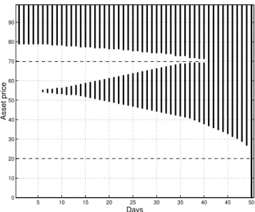
The structure of the optimal stopping domains for more complicated payoff functions than the standard payoff functions (1) and (2), such as, the piecewise linear payoff function given in Figure 2, is studied in the first part of the thesis. For this rather simple function the optimal stopping domains can have a more complicated structure than the stopping domains for the standard call payoff function (1) given in Figure 3. An example is given in Figure 5.
In particular, we give local conditions on the payoff functions such that the optimal stopping domains have the same one-threshold structure as the standard payoff functions’ stopping domains.
non-decreasing payoff functions, e.g., piecewise linear, stepwise, and quadratic. The price of the underlying asset follows the geometric random walk with log-normal increments given in (5) and the optimal stopping domains are generated by Monte Carlo simulations. The results show that the structure of the optimal stopping domains depends on the choice of payoff function. For the simplest piecewise linear payoff function (with two intervals with different slopes) the optimal stopping domains may have the structure shown in Figure 5. Also for a stepwise payoff function with M intervals with different constant payoff values the optimal stopping domains may be unions of M disjoint intervals. However, for the quadratic payoff function the structure of the optimal stopping domains is equivalent to the structure corresponding to the standard payoff function.
5 10 15 20 25 30 35 40 45 50 0 10 20 30 40 50 60 70 80 90 Days Asset price
Figure 5: An example of the structure of the optimal stopping domains
for a piecewise payoff function with two strike prices K1 and K2 in a
discrete time model where the option can be exercised at any moment n = 1, . . . , 50. The underlying asset follows a geometric random walk with log-normal increments.
In Paper A, we also present an analysis of classification errors. A classification error occurs when an asset value belonging to the optimal stopping domain is identified to be-long to the continuation domain, or the other way around, by the Monte Carlo algorithm. It is shown that the highest probability to make a classification error is for asset values close to the optimal stopping boundary and far away from the expiration date.
In Paper B, both theoretical and experimental studies of the structure of the optimal stopping domains for American type call options are presented. Sufficient local conditions,
connecting the payoff and the expected payoff from two sequential moments, for the optimal stopping domains to have a one-threshold structure are given. In the paper, the price process is a discrete time Markov process with multiplicative increments. The payoff functions are non-decreasing and convex. A sufficient condition for the existence of a one-threshold structure for a piece-wise linear payoff function is given explicitly. It is shown, by experimental results, that the one-threshold structure of the stopping domain can switch to a more complex structure, a union of two disjoint intervals, when the sufficient condition is violated.
In Paper C and Paper D, the results given in Paper B are extended, under the as-sumption that the underlying asset follows a general discrete time Markov processes, such that the asset value Sn at moment n is a function of the asset value at moment n − 1
and a random variable Yn, i.e., Sn = An(Sn−1, Yn), where An(x, y) is a deterministic
function. In these two papers the sufficient conditions for the stopping domains to have a one-threshold structure are given for convex payoff functions that are non-increasing (corresponding to put type options) and non-decreasing (call type options) in Paper C and Paper D, respectively.
Two examples are given where the conditions are applied to the standard linear payoff function and to a piecewise linear payoff function of a put option. In both examples the underlying asset follows either the binomial model or the geometric random walk with log-normal increments.
1.5.2 Convergence of the reward functions
In the last paper, Paper E, convergence results for the reward functions for discrete time optimal stopping problems corresponding to a family of American type options in discrete time markets are presented. The underlying price processes are inhomogeneous Markov processes and the payoff functions are time inhomogeneous monotone functions.
Using backward recursive analysis the paper studies the convergence of the reward functions, and the weak convergence of the reward processes and of the finite dimensional distributions of the reward processes, under the assumption that the transition probabil-ities of the price processes and the payoff functions depend on some “perturbation”, and converge to the corresponding “unperturbed” limit quantities as the perturbation tends to zero.
The paper ends with an application to an American type option in a continuous time Binomial market.
2
American type options and optimal stopping in
discrete time
Let us assume that the option can only be exercised at a finite number of moments n = 0, 1, ..., N until the expiration date. Despite American type options can be exercised at any time between 0 and the expiration, this assumption is reasonable. At any moment when the holder would like to exercise the option he must observe the price of the under-lying asset before making the decision. To assume that the holder can observe the price continuously is technically and economically not reasonable, since each observation takes time to do and costs some amount of money.
Let rn ≥ 0 be the riskless interest rate valid between moments n − 1 and n, n =
1, 2, ..., N . Throughout the thesis the interest rate will be deterministic.
We will denote the value of the underlying asset at moment n by Sn, n = 0, 1, ..., N .
The holder of an American type option can at each moment n decide whether to exercise, and receive the payoff g(Sn), or to hold the option until next moment n + 1. To
make the decision the holder has only the information available at moment n, and has no possibility to look into the future.
In the present section we formulate the optimal stopping problem and describe the so-lution procedure. A description of different approaches to valuate American type options is given in Section 2.5 to show the connection between the optimal stopping problem of the holder and the valuation of the option. In particular, the structure of the optimal stopping domains and the optimal stopping boundary are of importance for pricing Amer-ican type options. In Section 2.5 a review of the main results about the structure of the optimal stopping domains and the optimal stopping boundary is given. A review of the literature on the convergence of reward functions and option prices is given in Section 2.6. The present section ends with a description of the main problems studied in the thesis.
2.1
Markovian asset price evolution
Section 1.2 presented discrete time models for the price of the underlying asset based on the geometric random walk. These processes are all examples of Markov processes.
In this thesis we assume that the evolution of the price of the underlying asset follows a discrete time Markov process with a phase-space R+ = [0, ∞). Underneath our model
world, F is a σ-algebra of subsets of Ω, and P is a probability measure defined on F. A Markov process is a process with the so called Markovian property:
The future value Sn+1 of the process depends on the past values S0, S1, ..., Sn−1,
only through the present value Sn.
Thus, the transition probability that Sn+1 ≤ a, given the path of the past prices
S0 = s0, ..., Sn = sn, depends only on the present price Sn= sn, i.e.,
P {Sn+1 ≤ a|S0 = s0, ..., Sn= sn} = P {Sn+1 ≤ a|Sn = sn}. (8)
The Markov process is homogeneous in time (or stationary) if the transition probabil-ities are independent of n, i.e.,
P {Sn+1 ≤ a|Sn = s} = P {S1 ≤ a|S0 = s} , for n = 0, 1, . . . . (9)
In general, if the Markov process is homogeneous in time, we can describe the evolution of the process in the following dynamical form
Sn+1 = A(Sn, Yn+1), (10)
where A : R+× R → R+, A(x, y) is a measurable function and Y
1, Y2, . . . is a sequence of
independent identically distributed real-valued random variables. One example of A(x, y) is the multiplicative function
Sn= A(Sn−1, Yn) = Sn−1Yn,
where Y1, Y2, . . . is a sequence of non-negative real-valued random variables. That is, the
prices follows a geometric random walk. If Yn is log-normal, then we have the geometric
random walk given in (5).
If the transition probability given in (8) depends on n, the Markov process is said to be time inhomogeneous (or non-stationary). Time inhomogeneous Markov processes can be described in the dynamical form
Sn+1 = An+1(Sn, Yn+1), (11)
where An : R+× R → R+, An(x, y) is a measurable function and Y1, Y2, . . . is a sequence
2.2
Time inhomogeneous and non-standard payoff functions
As seen in Section 1.1 the payoff functions for standard American options, (1) and (2), are fixed during the life time of the option.
Throughout the thesis we assume that the payoff functions of the options are time inhomogeneous, that is, they can change with time, and denote the payoff function at moment n, n = 0, 1, ..., N , by
gn : R+ → R+.
In particular we study general non-negative and monotone payoff functions.
Example 3. Time inhomogeneous standard American call payoff functions. For the standard American call option we can let the strike price K vary over time such that the payoff function will be
gn(s) = [s − Kn]+,
where Kn is the strike price at moment n.
Another way of modifying the payoff function is to multiply the standard payoff func-tion with a time varying coefficient an> 0 such that
gn(s) = an[s − K]+.
We can, of course, combine these two cases such that
gn(s) = an[s − Kn]+. (12)
Equivalent modifications of the put payoff function (2) can be made.
We can also consider other types of payoff functions than the standard payoff functions given in (1), (2) and the modified time inhomogenous versions given in Example 3. Example 4. Time inhomogeneous piecewise linear payoff functions. A piecewise linear payoff function for an American type call option can have the following form
gn(s) = 0, if s ≤ Kn,1, an,1(s − Kn,1), if Kn,1 < s ≤ Kn,2, an,1(Kn,2− Kn,1) + an,2(s − Kn,2), if s ≥ Kn,2, (13)
where an,1 and an,2 are non-negative and 0 ≤ Kn,1 ≤ Kn,2 are the strike prices.
Figure 2 shows an example of a piecewise linear payoff function for a call option with strike prices Kn,1 = 30 and Kn,2 = 70 and coefficients an,1 = 1 and an,2 = 3/2.
An American type put option can have a piecewise linear payoff function such as gn(s) = an,1(Kn,1− s) + an,2(Kn,2− Kn,1), if 0 ≤ s ≤ Kn,1, an,2(Kn,2− s), if Kn,1 ≤ s ≤ Kn,2, 0, if s > Kn,2. (14)
Note that the piecewise linear payoff functions (13) and (14) can be interpreted as the payoff of a portfolio of two options of the same type written on the same underlying asset, with different strike prices, exercised simultaneously. In this case, for the call option an,1 and an,2− an,1 is the number of units of the option with strike price Kn,1 and Kn,2,
respectively, in the portfolio. For the put option, an,1 − an,2 and an,2 is the number of
units of the option with strike price Kn,1 and Kn,2, respectively, in the portfolio.
We can, of course, have piecewise linear payoff functions with more than two strike prices, i.e., portfolios with more than two options.
2.3
Optimal stopping
2.3.1 Formulation of the problem
The problem of finding the optimal moment to exercise the option is a discrete time optimal stopping problem. We are given a set of moments {0, 1, . . . , N } where we can chose to stop or to continue one step more. At each moment n we observe the price of the underlying asset and make a decision to stop or to continue. If we stop at moment n and exercise the option we receive the payoff gn(sn). If we continue, we make a new
observation at moment n + 1.
In the optimal stopping problem we would like to find the optimal moment τopt to
exercise such that the expected present value of the payoff is maximized. Hence, we would like to maximize, over all admissible exercise moments τ , the functional
Φg(τ ) = Ee−Rτgτ(Sτ), (15)
where Rτ = r1+ ... + rτ is the accumulated risk free interest rate up to moment τ .
2.3.2 Stopping times
We first have to describe the admissible exercise moments.
A stopping time, or a finite Markov time, τ for the price process (Sn) is a finite positive
The event {τ = n} is determined by the random variables S0, ..., Sn only.
That is, the event {ω : τ (ω) = n} ∈ σ[S0, S1, . . . , Sn], where σ[S0, S1, . . . , Sn] is the
σ-algebra generated by the path of the price process up to moment n.
Thus, we can only use the information available at moment n to decide if τ = n. We are not allowed to look into the future.
The optimal moment to stop is found in the class of all stopping times for the price process (Sn) less than or equal to N . Denote by M0,N the class of all admissible stopping
times for the process (Sn) less than or equal to N . That is, M0,N is the class of all
stopping times τ such that for all ω ∈ Ω, 0 ≤ τ (ω) ≤ N , and for every n, the event {ω : τ (ω) = n} ∈ σ[S0, S1, . . . , Sn].
Hence, the optimal stopping time τopt maximizing (15) is given by
Φg(τopt) = sup τ ∈M0,N
Ee−Rτg
τ(Sτ). (16)
2.3.3 Backward induction, optimal stopping domains, and optimal stopping time
Backward induction (or dynamic programming) is usually used to solve the maximization problem (16), see, e.g., Chow, Robbins, and Siegmund (1971), and Shiryaev (1978).
We begin by defining the optimal strategy at moment N , the expiration date. Since the option will be worthless after the expiration date the optimal strategy will be defined as follows. If the payoff gN(s) is greater than zero, then the option is exercised. If the
payoff is zero then the option is thrown away without being used. Thus, whatever happens we stop.
After we have defined the optimal strategy at N we take one step backwards in time to moment N − 1. To find the optimal strategy at moment N − 1, we compare the value of the payoff if the option is exercised at N − 1 with the expected discounted value of the optimal strategy defined for moment N . If the payoff is greater than or equal to the expected discounted value of the optimal strategy at moment N , it is optimal to stop. Otherwise, we should continue to N and follow the optimal strategy already defined.
Thus, we can by this procedure divide the asset prices at moment N − 1 into two sets, the optimal stopping domain and the continuation domain.
Let us assume that we have already found the optimal strategies for n+1, ..., N −1, N . To find the optimal strategy at moment n, we compare the payoff if the option is exercised immediately with the expected discounted value of the optimal strategy already found for
moment n + 1. If the payoff is greater than or equal to the expected discounted value of the optimal strategy at n + 1, it is optimal to stop. Otherwise, it is better to continue until n + 1 and follow the optimal strategy for n + 1.
We define the reward function wN −n(s) at moment n to be the value of the optimal
strategy at moment n given that the asset price Sn = s. If it is optimal to exercise
the option at moment n for the asset price Sn = s, then wN −n(s) = gn(s). Otherwise,
the reward function is equal to the expected discounted value of the optimal strategy at moment n + 1 given that Sn= s.
Consequently, the set of asset prices such that it is optimal to stop at moment n, the so-called optimal stopping domain for moment n, is defined by
Γn = {s ≥ 0 : wN −n(s) = gn(s)},
i.e., the set of asset prices at moment n such that the value of the optimal strategy is equal to the payoff.
The complement to the optimal stopping domain is the continuation domain ΓC
n = R +\ Γ
n= {s ≥ 0 : wN −n(s) > gn(s)},
i.e., the set of asset prices at moment n such that the value of the optimal strategy is strictly greater than the payoff.
As said above, we begin the backward induction with defining the optimal strategy at moment N . This is the expiration date and since the option will not exist after N we define the value of the optimal strategy to be equal to the payoff of the option for all asset prices. That is, we define the reward function w0,
w0(s) = gN(s),
for all s ≥ 0. Consequently, the optimal stopping domain ΓN = [0, ∞).
Note that the optimal stopping domain at the expiration date includes all values of the underlying asset. This should not be interpreted as the option is exercised at the expiration date regardless of the value of the underlying asset. The option should, of course, only be exercised if the payoff gN(SN) is greater than zero. Otherwise the option
should be thrown away without being used. Thus, the optimal stopping domain is not equal to the exercise domain at the expiration date.
To find the optimal strategy at moment N − 1 we compare, for every s ∈ [0, ∞), the payoff if we exercise the option gN −1(s) with the conditional expected discounted reward
at moment N given that SN −1 = s. Hence, for every s ∈ [0, ∞), the reward function is
defined by
w1(s) = max©gN −1(s), E[e−rNw0(SN)|SN −1 = s]ª ,
where rN ≥ 0 is the risk free interest rate valid between N − 1 and N .
The optimal stopping domain at moment N − 1 is by definition
ΓN −1 = {s : w1(s) = gN −1(s)} =©s : E[e−rNw0(SN)|SN −1 = s] ≤ gN −1(s)ª .
After finding the optimal strategy at moment N − 1 we continue to moment N − 2. For each asset price s ∈ [0, ∞) we compare the value of the payoff gN −2(s) if we exercise
the option with the expected discounted value of holding the option until moment N − 1 and follow the optimal strategy already defined for moment N − 1 given that SN −2 = s.
We will, therefore, have the following reward function
w2(s) = max©gN −2(s), E[e−rN −1w1(SN −1)|SN −2 = s]ª ,
where w1(SN −1) = gN −1(SN −1) if SN −1 ∈ ΓN −1, and w1(SN −1) = E[e−rNw0(SN)|SN −1] if
SN −1 ∈ ΓCN −1.
The optimal stopping domain at moment N − 2 is by definition ΓN −2 = {s : w2(s) = gN −2(s)} .
By continuing this induction reasoning we can define the reward functions and the optimal stopping domains for all moments N − 3, ..., 1, 0.
By construction, the reward function at moment 0 is the value of the optimal strategy at moment 0, given that the price process starts at s0.
Hence
wN(s0) = Φg(τopt).
Furthermore, the optimal stopping time is given by
τopt = min{0 ≤ n ≤ N : Sn∈ Γn}, (17)
that is, τopt is the first moment the asset price enters the optimal stopping domain (see,
e.g., Chow, Robbins, and Siegmund (1971) and Shiryaev (1978)). Hence, the optimal stopping time is a so called first hitting time or first passage time.
The first hitting time structure of the optimal stopping time implies that at any moment n, the optimal decision to stop and exercise or to wait should be based on the value Sn only and should not depend on the past values S0, ..., Sn−1.
Note that the reward process (wN −n(Sn)) is the Snell envelope of the discounted
payoff process ¡e−Rng
n(Sn)¢, that is, it is the smallest supermartingale (Zn) such that,
for every n, Zn≥ e−Rngn(Sn). (A discrete time Markov process (Zn) is a supermartingale
if E{Zn+1|Z0, . . . , Zn} ≤ Zn.)
Denote by Mn,N the class of all admissible stopping times for the process (Sn) such
that n ≤ τn ≤ N . From the general theory of optimal stopping we also have that
wN −n(Sn) = ess sup τn∈Mn,N E £e−Rτng τn(Sτn)| Sn ¤ (P −a.s.), (18) where Rτn = r1+ . . . + rτn.
The essential supremum of a family M of random variables defined on (Ω, F, P ) is a random variable η = ess supξ∈Mξ such that: (a) P (η ≥ ξ) = 1 for all ξ ∈ M; (b) if ˜η is
another random variable such that P (˜η ≥ ξ) = 1 for all ξ ∈ M, then P (˜η ≥ η) = 1. Moreover, the optimal stopping time τn maximizing (18) exists and is given by
τn= min{n ≤ k ≤ N : Sk ∈ Γk}.
As shown above, the optimal stopping domains are defined using the reward func-tions. However, the definition is too inexplicit and gives no information about the actual structure of the optimal stopping domains. Thus, we cannot, for example, describe how the structure depends on the properties of the payoff functions.
2.4
Pricing of American options
To find the fair price of an American type option the early exercise feature has to be taken under consideration. This makes the valuation of American type options much more complicated than the valuation of European options, since in the latter case the option can be exercised at maturity only.
This section gives a short review of the basic approaches to price American type options, without any attempt to be complete. The main idea is to show the connection between the optimal stopping theory presented above and the valuation of the options. The section begins with a summary of some of the main principles of pricing financial derivatives to initiate those readers whom are not familiar with the theory.
There are several books on the subject of mathematical finance and pricing of fi-nancial derivatives, for example, Pliska (1997), Shiryaev (1999), Karatzas and Shreve (2001), Bj¨ork (2004), F¨ollmer and Schied (2004), Shreve (2004a, 2004b), and Musiela and Rutkowski (2005).
2.4.1 Risk-neutrality
A key concept in valuation of any financial derivative is that the fair price should not create arbitrage opportunities. Arbitrage opportunities are defined using so called self-financing strategies. A trading strategy is a strategy used by an investor to rebalance an investment portfolio consisting of the assets traded on the market. A self-financing trading strategy is a trading strategy where no money is added to or withdrawn from the portfolio during the lifetime of the investment. Hence, any changes in the portfolio’s value during the lifetime of the investment is due to a gain or a loss in the investment.
Let πN be a self-financing trading strategy with maturity at moment N , and let VnπN
denote the value of πN at moment n. The trading strategy πN is said to be an arbitrage
opportunity at moment N if (i) VπN 0 = 0; (ii) VπN N ≥ 0 (P − a.s.); (iii) P (VπN N > 0) > 0.
Thus, a self-financing trading strategy is an arbitrage opportunity if starting with zero value the portfolio has a nonnegative value at the maturity of the investment with probability one, and with positive probability the value is positive.
The First fundamental asset pricing theorem gives the necessary and sufficient condition for a market to be arbitrage-free:
A financial market is arbitrage-free if and only if there exists a risk-neutral (or equivalent martingale) probability measure.
A risk-neutral probability measure Q, also called an equivalent martingale measure, is a transformation of the original (historical) probability measure P such that it is equivalent to P and the discounted price process ¡e−RnS
n¢ is a martingale under this transformed
measure, i.e., EQ{e−Rn+1Sn+1| e−RnSn} = e−RnSn for all n. (Two probability measures
if and only if Q(A) = 0, A ∈ F, i.e., the two measures agrees about which events are improbable. A discrete time Markov process (Zn) is a martingale if, for every n,
E{Zn+1|Z0, . . . , Zn} = Zn.)
Note that the First fundamental asset pricing theorem does not say anything about the uniqueness of the risk-neutral probability measure.
The uniqueness of the risk-neutral probability measure is closely related to the concept of completeness of a financial market. Before defining what it means that a market is complete we need the notion of attainable or marketable contingent claims.
A contingent claim XN is a random variable that represents the payoff at time N
of some financial contract (e.g. an European type option) with maturity N . A contin-gent claim is attainable or marketable if there exists a self-financing trading strategy πN
replicating the contingent claim, that is, at maturity N , VπN
N = XN (P − a.s.).
We can now define what a complete market is:
A financial market is complete if every contingent claim can be replicated. A market that is not complete is said to be incomplete.
An example of a complete discrete time model is the Binomial model, and a complete continuous time model is the geometric Brownian motion. The trinomial tree model is an example of an incomplete discrete time model.
The Second fundamental asset pricing theorem gives the necessary and sufficient condition for the uniqueness of the risk-neutral measure:
A financial market is complete and arbitrage-free if and only if there exists a unique risk-neutral (or equivalent martingale) probability measure.
Thus, in an incomplete arbitrage-free market there are more than one risk-neutral probability measure. Let P(P ) denote the collection of risk-neutral probability measures equivalent to P .
In an incomplete market the contingent claim is attainable if and only if the expected discounted payoff at moment N , EQe−RNXN, takes the same value for every risk-neutral
probability measure Q ∈ P(P ).
For American type options the question about attainability becomes more complicated since we have to create a self-financing strategy that replicates the payoff of the option for any admissible stopping moment τ . The following is however true:
An American option is attainable if and only if, for every admissible stopping time τ , the expected discounted payoff EQe−Rτgτ(Sτ) takes the same value for
every risk-neutral probability measure Q ∈ P(P ).
That is, the option is attainable if and only if there exists a unique arbitrage-free price. Since this holds if there exists only one risk-neutral probability measure, every American option is attainable in a complete market.
2.4.2 The arbitrage pricing method
One approach to value an American type option is to use a hedging strategy, i.e., invest-ment and consumption strategy that replicates the payoff of the option. This approach is based on the seller’s ability to protect himself from future liabilities to the option holder. It is important that the constructed strategy replicates the option’s payoff at any admis-sible stopping time τ . Since the strategy replicates the option’s payoff, the option and the strategy must have the same value at any time. Otherwise there would exist an arbitrage opportunity.
2.4.3 The optimal stopping strategy of the holder
Another approach is to solve the optimal stopping problem of the holder of the option, i.e., to find the holder’s optimal exercise strategy.
The arbitrage-free price of the American option in a complete market is in this case found by solving the optimal stopping problem
Φg(τopt) = sup τ ∈M0,N
EQe−Rτgτ(Sτ), (19)
where the expectation is with respect to the unique risk-neutral probability Q.
Therefore, since wN(s0) = Φg(τopt) and the reward functions are defined recursively,
wN(s0) is the time zero value of the option if the expectations in the reward functions are
with respect to the unique risk-neutral probability measure.
Moreover, the discounted value of the option at moment n is given by the Snell envelope wN −n(Sn) = ess sup
τn∈Mn,N
EQ £e−Rτngτn(Sτn)| Sn
¤
(Q − a.s.), (20)
under the condition that the expectation is with respect to the unique risk-neutral prob-ability measure Q.
Pricing an American option that is not attainable in an incomplete market becomes more complicated, since there exists no unique risk-neutral probability measure and no unique arbitrage-free price. Instead we have a collection of arbitrage-free prices.
We can at least say that the time zero value of the option will be less than or equal to the upper price
sup
Q∈P(P )
sup
τ ∈M0,N
EQe−Rτgτ(Sτ)
and greater than or equal to the lower price inf
Q∈P(P ) τ ∈Msup0,N
EQe−Rτgτ(Sτ).
In continuous time models the continuous time optimal stopping problem (19) can by formulated as a free boundary value problem using partial differential equations.
In the free boundary value method, the value of the American option is defined in two different ways depending on whether the value of the underlying asset is in the stopping region or in the continuation region. In the stopping region the option is exercised and the value is equal to the payoff. In the continuation region the option is alive and the value is given by a partial differential equation.
By solving the partial differential equation under suitable terminal and boundary conditions, the value of the (live) American option can be determined as a function of the early exercise boundary. Unfortunately the boundary is unknown (that is why it is called the free boundary value problem) and, therefore, has to be found simultaneously as solving for the value of the option.
2.4.4 The early exercise premium representation
The connection between the value of an American option and the early exercise boundary (and the optimal stopping domains) are clearly visible in the so called early exercise premium representation of the American option’s value.
The representation, given in Kim (1990), Jacka (1991), and Carr, Jarrow, and Myneni (1992), expresses the value of the American call (put) option as the sum of the value of an European call (put) option and the so called early exercise premium, i.e.,
CAM(St, dt, K, T ) = CEU(St, K, T ) + e(St, dt), 0 ≤ t ≤ T,
where CAM(St, dt, K, T ) is the value of the American call, CEU(St, K, T ) is the value of
and expiration date T as the American option, and e(St, dt) is the early exercise premium.
The early exercise premium is a function of the early exercise boundary dt and the value
of the underlying asset St. However, since the early exercise boundary is unknown, it is
defined implicitly by a recursive integral equation.
In Salminen (1999), the early exercise premium representation for standard American put options is derived using an alternative technique, developed in Salminen (1985), and based on the representation theory of excessive functions.
A discrete time version of the early exercise premium representation for a discrete time standard American put option is derived in Iwaki, Kijima, and Yoshida (1995), when the underlying price process is a Markov process with time homogeneous independent increments.
2.4.5 Numerical approximations
Since there is a lack of analytical solutions of the value of American options several differ-ent types of numerical procedures to solve the problem have been proposed, e.g., binomial or multimnomial tree methods, finite difference methods and Monte Carlo methods. We refer to Broadie and Detemple (1996), Rogers and Talay (1997), Kwok (1999), Glasserman (2003), and Hull (2006), for a review of numerical methods in finance.
The Monte Carlo method is the approach to approximate the maximization problem in (16) best fitted in the context of the present thesis. Due to its flexibility the Monte Carlo method is very useful. We can, for example, use it to investigate options with complicated payoff functions or complicated price processes. Using Monte Carlo methods we can also estimate the average exercise time, the probability of early exercise, the probability that the option is ever exercised and other characteristics concerning holding the option.
The critical point in valuing American options with Monte Carlo methods is, just as for any other method, that it is necessary to know the structure of the optimal stopping domains and the optimal stopping boundary.
See Boyle, Broadie, and Glasserman (2001), and Glasserman (2003) for recent re-views of Monte Carlo methods in option pricing. See also and Basso, Nardon, and Pi-anca (2002a) and the references therein. Examples of Monte Carlo algorithms using the knowledge of the structure of the optimal stopping domains can be found in Silvestrov, Galochkin, and Sibirtsev (1999) and Silvestrov, Galochkin, and Malyarenko (2001).
2.5
Structure of the optimal stopping domains
In Section 2.4 we saw that the valuation of American type options implies studies of the structure of the optimal stopping domains and the properties of the early exercise boundary.
In this section we will give a short review of the main results known about the optimal stopping domains and the optimal stopping boundaries of American type options.
Most of the results about the structure of the stopping domains and the early exercise boundary are based on continuous time models.
2.5.1 Standard American options
The two main properties known about the optimal stopping domains for standard Amer-ican call options (see Example 1) are:
C1. Up-connectedness: if s ∈ Γt, then s0 ∈ Γt for every s0 ≥ s.
C2. Right-connectedness: if s ∈ Γt, then s ∈ Γt0 for every t0, 0 ≤ t ≤ t0 ≤ N.
Up-connectedness means that if an asset price at moment t is in the optimal stopping domain, then all asset prices above this asset price are also in the optimal stopping domain. This property is presented in Broadie and Detemple (1999) for an asset price evolution based on a (risk-neutral) geometric Brownian motion.
Note that the up-connectedness property is imposed on the optimal stopping domain by the definition of the early exercise boundary used in the free boundary formulation given in Section 2.4.4. In Broadie and Detemple (1999), this property is proved using the arbitrage pricing method with consumption and investment portfolios.
Right-connectedness means that if an asset price s at moment t is in the optimal stopping domain Γt, then s is in the optimal stopping domains for all moments t0, such
that t ≤ t0 ≤ N . This property is presented in Broadie and Detemple (1999) for a
(risk-neutral) geometric Brownian motion.
The right-connectedness property can be formulated in the following equivalent ways for any moments t and t0, such that 0 ≤ t ≤ t0 ≤ N :
Γ0 ⊆ Γt ⊆ Γt0 ⊆ ΓN and ΓC0 ⊇ ΓC t ⊇ Γ C t0 ⊇ Γ C N.
In discrete time this property, known from the general theory of discrete time optimal stopping (see Shiryaev (1978)), holds for time homogeneous Markov chains and can be expressed as
Γ0 ⊆ Γ1 ⊆ . . . ⊆ ΓN
and
ΓC
0 ⊇ ΓC1 ⊇ . . . ⊇ ΓCN.
In fact, this is true for homogeneous Markov chains which can take any value in the phase space at every moment n = 0, 1, . . . , N . (See the discussion below about the stopping domains for the American put option in the Binomial model.)
The following two properties for the optimal stopping boundary are interesting: C3. The optimal stopping boundary is non-increasing in time, i.e., for every t and t0
such that 0 ≤ t ≤ t0 ≤ N :
d0 ≥ dt≥ dt0 ≥ dN.
C4. If the model of the underlying asset has continuous (in time) trajectories, then the optimal stopping boundary dt is continuous in time.
Property C3, the optimal stopping boundary is non-increasing, is presented in Van Moerbeke (1976) for a geometric Brownian motion and in Kim (1990) for a risk-neutral geometric Brownian motion.
The non-increasing property of the optimal stopping boundary is equivalent to the right-connectedness of the optimal stopping domain, property C2, if property C1 holds.
Property C4 is presented in Van Moerbeke (1976) (it is actually proved that the boundary was continuously differentiable) and in Kim (1990). The continuity of the stopping boundary follows from the continuity of the trajectories of the price of the underlying asset, hence, the continuity of the optimal stopping boundary is, of course, only true for continuous time models with continuous trajectories such as the geometric Brownian motion.
The up- and right-connectedness properties of the optimal stopping domains and that the optimal stopping boundary is non-increasing for standard American call options are illustrated in Figure 3 for a discrete time geometric random walk with log-normal incre-ments.
The two main properties known about the optimal stopping domains for standard American put options (see Example 2) are:
P1. Down-connectedness: if s ∈ Γt, then s0 ∈ Γt for every s0 ≤ s.
P2. Right-connectedness: if s ∈ Γt, then s ∈ Γt0 for every t0, 0 ≤ t ≤ t0 ≤ N.
The down-connectedness follows from the definition of the early exercise boundary used in the free boundary formulation (see Merton (1973)). The down-connectedness of the optimal stopping domain is proved in Jacka (1991) by showing that the continuation domain is up-connected.
The right-connectedness is equivalent with property C2 for call options (see Kim (1990)).
The following two properties of the optimal stopping boundary for American put options are interesting:
P3. The optimal stopping boundary is non-decreasing in time, i.e., for every t and t0
such that 0 ≤ t ≤ t0 ≤ N :
d0 ≤ dt≤ dt0 ≤ dN.
P4. If the model of the underlying asset has continuous (in time) trajectories then the optimal stopping boundary dt is continuous in time.
The non-decreasing property of the optimal stopping boundary is presented in van Moerbeke (1976), Kim (1990), Jacka (1991), see also Myneni (1992).
The continuity property is presented in van Moerbeke (1976), see also Jacka (1991) and Myneni (1992), and is identical to property C4 for American call options.
The properties of the optimal stopping domains and the optimal stopping boundary of a standard American put option are illustrated in Figure 4 for a discrete time geometric random walk with log-normal increments.
Other results about properties of the optimal stopping boundary can be found in Barles, Burdeau, Romano, and Samsœn (1995), Kuske and Keller (1998), Touzi (1999), Evans, Kuske, and Keller (2002), and Ekstr¨om (2004). In Ekstr¨om (2004), for example, the stopping boundary for a standard American put option is proved to be convex in time, as the underlying asset follows a risk-neutral geometric Brownian motion.
In this context we would like also to mention the paper by Janson and Tysk (2003) where continuity, monotonicity, and convexity properties of option prices are studied.
For the binomial model the up-connectedness or down-connectedness exists. However, the boundary is in general not non-increasing or non-decreasing, i.e., neither dn ≥ dn+1
price at moment n + 1 can take only two values, either Sn+1 = uSn or Sn+1 = dSn, where
0 < d ≤ 1 ≤ u. In the paper by Kim and Byun (1994), the optimal exercise boundary for an American put option in a Binomial model is studied. They show that the optimal exercise boundary is non-decreasing as the option approaches the expiration date, but there exist saw-toothed shapes superimposed in the general increase. Their results imply that one and only one of the following is true for n = 2, . . . , N : 1) dn−2 = dn > dn−1; 2)
dn−2 = dn < dn−1; 3) dn−2 < dn−1 < dn. Hence, the right-connectedness property does
not necessarily hold.
2.5.2 Dividends and the optimal stopping domains
In this section we will describe some results known about the structure of the early exercise regions for the standard American option, i.e., an option with the time homogeneous payoff functions given in (1) and (2), if the underlying asset pays dividends.
For the American call option written on an underlying asset paying continuous div-idends with constant dividend yield, the structure of the optimal stopping domains has the properties described above, i.e., up- and right-connectedness with non-decreasing and continuous (if continuous model) boundary. See, e.g., Merton (1973), Kim (1990), Jacka (1991), Broadie and Detemple (1999).
In fact, if the underlying asset does not pay dividends and the interest rates are posi-tive, then the American call option will not be exercised optimally before the expiration date. The result follows from the fact that the value of the American call is strictly larger than the value of the payoff [s − K]+ for any value s ≥ 0 of the underlying asset in this
case. And since the option will be optimally exercised only for those values of the under-lying asset such that the value of the option is equal to the payoff, the option will never be optimally exercised earlier than the expiration date. (To see this in a complete discrete time model, use the fact that¡e−RnS
n¢ is a Q-martingale and that 0 ≤ Rn≤ Rn+1 for all
n, to prove that EQ[e−Rn+1(Sn+1− K)+|e−RnSn] ≥ e−Rn(Sn− K)+. Consequently, by the
definition of the reward functions wN −n(s) = EQ[e−rn+1wN −n−1(Sn+1)|Sn = s]. Hence,
τopt = N and Φ(τopt) = wN(s0) = EQ[e−RN(SN − K)+|S0 = s0]. Note that we here
consider the problem of optimal stopping under the risk-neutral probability measure. For a more detailed discussion, see, e.g., Merton (1973), Pliska (1997), Kwok (1999), F¨ollmer and Schied (2004), Hull (2006).)
This result implies that if the value of the underlying asset is significantly above the strike price, i.e., the option is deep-in-the-money, and the holder believes that the value
will fall until the expiration date, then it is better to sell the option than to exercise it. Hence, there will exist optimal stopping domains based on the holder’s personal market view and these domains will give recommendations for the holder to stop owning the option. The practical decision to either sell or exercise should be based on what is generating the largest profit.
Finally, in the case of discretely payed dividends, the American call option could be optimally exercised just prior to the ex-dividend dates, i.e., just before the dividend is payed, if the dividend is sufficiently large relative to the strike price, the value of the underlying asset is above the exercise boundary and the ex-dividend date is close to the expiration date (see, e.g., Kwok (1999)). Once again we point out that there exist optimal stopping domains based on the holder’s preferences and that these domains will give the recommendation to stop owning the option.
For an American put option written on an underlying asset paying continuous divi-dends with constant dividend yield, the structure of the optimal stopping domains and the early exercise boundary are equivalent to the structure corresponding to an American put option written on an underlying asset without dividend payment. That is, properties P1 - P4 hold in both cases. See, e.g., Kim (1990), Jacka (1991), Broadie and Detemple (1999), Basso, Nardon, and Pianca (2002a, 2002b).
In the case of discretely payed dividends, the American put option is most likely to be exercised at ex-dividend dates, i.e., just after the dividend is payed, or just prior to the expiration date, or at very low values of the underlying asset (see Geske and Shastri (1985), Omberg (1987) and Meyer (2002)).
Again the optimal stopping domains based on the holder’s preferences will give rec-ommendations to stop holding the option. And these optimal stopping domains will not necessarily coincide with the early exercise regions, just as in the two cases for the call option mentioned above.
However, the optimal stopping problem where we consider both early exercise and re-selling of the option is much more complicated, since we in this case have a two dimensional optimal stopping problem. Furthermore, we have to create a stochastic model not only for the value of the underlying asset but also for the market price of the option, since the market price of the option could deviate from the theoretical price. The optimal stopping problem considering both early exercise and re-selling is a problem for future research.