Data Dependency Analysis in Industrial Systems

(1)

Data Dependency Analysis in Industrial

Systems

Mälardalen University

School of Innovation, Design and Engineering Azra Čaušević

DVA423 Thesis for the Degree of Master of Science (60 credits) in Computer Science with Specialization in Software Engineering, 15 credits

2015-10-28

Examiner: Jan Carlson

(2)

1

Abstract

Software in modern industrial systems may have complex data dependencies. As a result of this, it can be hard for system developers to understand the system’s behavior, if they cannot explicitly see these dependencies. This thesis addresses this problem, with an emphasis on dependencies among data in systems built using the IEC 61499 standard. An analysis method was developed, with which we are able to extract data dependency information from basic and composite function blocks. The first step of handling this problem is to investigate how the data dependencies occur in IEC 61499. The second step is to create a formal definition of IEC 61499 elements that were needed in order to formulate the analysis method. Next, we define a dependency matrix, in which we store the information regarding dependencies between input and output data ports. Later, we formulate the necessary algorithms for data dependency analysis in basic and composite function blocks. Finally, the last piece of the puzzle is to develop a plug-in for Framework for Distributed Industrial Automation and Control – Integrated Development Environment. This plug-in is used to show that the analysis method is efficient and that the proposed analysis is applicable to IEC 61499 systems.

(3)

2

List of Figures

2.1 PL defined in IEC 61131-3 implementing a simple function ... 7

2.2 A Basic Function Block ... 9

2.3 A Function Block Network... 10

3.1 Research Method ... 12

5.1 ECC of FB_FT_TN16 FB... 17

5.2 (a) BFB interface (b) ECC BFB... 19

5.3 Stages of the Dependency Matrix... 21

5.4 Stages of the Dependency Matrix... 21

5.5 CFB analysis example ... 25

5.6 Dependency matrices of BFBs F_1 and F_2 ... 25

5.7 Stages of updating dependency matrix of CFB ... 26

5.8 Executing the plug-in ... 28

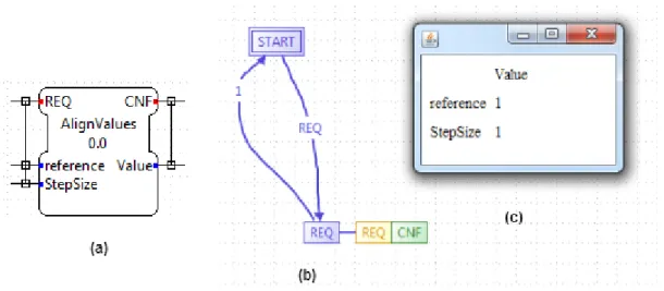
5.9 BFB AlignValues (a) interface (b) ECC (c) dependency matrix ... 28

5.10 Launching the 4DIAC-IDE ... 29

6.1 Interface of FB_FT_TN1 BFB ... 30

6.2 ECC of FB_FT_TN1BFB ... 30

6.3 Dependency matrix of the BFB FB_FT_TN1 ... 31

6.4 Dependency Matrix extended with internal variables ... 32

6.5 Interface of Int_To_LReal ... 32

6.6 Composite Network of Int_To_LREAL CFB ... 33

6.7 Results of Data Dependency Analysis in CFB INT_To_RLeal ... 33

6.8 Interface of LReal_To_Int CFB ... 34

6.9 Composite Network of CFB LReal_To_Int ... 34

(5)

4

1. Introduction

Over the last years manufacturers of distributed automation systems use programming languages that are defined in the IEC 61131-3 standard, in order to program the fundamental controller of the systems, namely programmable logic controllers (PLCs). The increased usage of controllers, in conjunction with the rapid improvement of the network performance, had as a result the increased complexity of the distributed applications [20]. In order to tackle this, IEC established the 61499 standard. The purpose of this standard is to deal with new requirements of the distributed applications, such as configurability interoperability and others [20]. Nowadays the standard is commonly used in order to define software components of automated systems [20].

The fundamental software unit defined in the 64199 standard is the function block [21]. According to the events that are triggered, the function block executes specific algorithms which leads to the production of new events and data. The data transfer is achieved through the data inputs and outputs that are defined on the interface of each function block [21].

Despite the fact that the research regarding the standard is quite extensive, a field that has not been investigated thoroughly is related to the dependency between data inputs and outputs of a function block.

This thesis will deal with this matter.

1.1 Problem formulation

The main goal of the thesis is to develop the theory of an analysis method, with which we will be able to investigate the dependencies between data in industrial software systems. Based on this theory we will be able to examine software data flow. This will allow us to study how program outputs depend on program inputs. In addition, the theory will provide us a way for exploring which inputs a selected output depends on. Furthermore, the formulated theory will illustrate the way we should follow in order to identify how many and which outputs depend on a specific input.

In this thesis we will consider systems that are built using the IEC 61499 standard. Investigating the answers to the following research questions will provide us with the needed information in order to reach the above mentioned goal:

RQ1: In which ways can output data be dependent on input data based on the IEC 61499 standard?

RQ2: Which method can we use for calculating data dependency?

The second main goal of this thesis is to implement a plug-in for the 4DIAC-IDE tool. 4DIAC is an open and free framework that gives the opportunity to establish an automation and control environment based on the three main targets, namely portability, configurability and interoperability. The implemented prototype will be used in order to validate the theoretical analysis definition we formulated previously.

(6)

5

This thesis report is organized as follows. In Section 2 we provide the necessary theoretical information regarding used standard and framework that is needed in order to understand the contributions of the report. In Section 3 we describe the research method that was used to retrieve the results of the work, while in Section 4 we provide formal definition of IEC 61499 elements that are required to present the results of the work. Section 5 presents formulated data dependency analysis method and guidelines for developed plug-in usage. In Section 6 we evaluate the results of the research by executing formulated analysis on existing industrial systems. Finally in Section 7 we summarize the results of the research and we discuss future work.

Foundation for this thesis is a previous project, partly funded by ABB, where a new method for analyzing control dependencies in systems implemented in IEC 61499, was developed.

(7)

6

2. Background

This chapter describes fundamental theoretical principles, in order for the reader to understand this scientific report. Section 2.1 outlines the International Electrotechnical Committee (IEC) 61131-3 standard, while the following section 2.2 describes its successor namely the IEC 61499 standard. Next, Function Blocks (FBs) with a focus on data ports are illustrated in section 2.3. Finally, section 2.4 presents Framework for Distributed Industrial Automation and Control (4DIAC) for which the additional plug-in was created.

2.1. The IEC 61131-3 standard

Nowadays, the process of designing a distributed automation system is quite complicated. The reason is that the distributed automation system is composed of a wide variety of control nodes with multiple interactions. Programmable logic controllers are mainly used in order to implement the control nodes.

PLCs contain programmable memory in which all the necessary instructions and data are stored to enable PLCs to implement their tasks [8]. The instructions are written in a specific programming language and can be seen as a set of orders which guide the PLCs how to execute their tasks. Moreover, all the required functions are stored in the memory of PLCs. These functions are needed in order for the PLCs to perform logic, timing or arithmetic operations etc. [8]. One of the major advantages of the PLC is its reusability. It is possible to reuse the same PLC in different distributed automation systems which makes a PLC cost effective [8].

The main problem that was needed to be addressed in the beginning of the PLC development was that there wasn’t a globally defined programming language that could be used in order to develop PLCs [8]. Different manufacturers were developing PLCs by using their own programming languages. As a result of this, the significant advantage of PLC, reusability, tended to be diminished. It was not possible to reuse a PLC in more than one distributed automation systems because the programming language in which it was developed was different. As a consequence of this, PLC development became costly and time consuming [5]. Therefore, it became clear that a set of standardized programming languages that could be used for the development of PLCs was needed. Thus the 61131-3 standard was established by IEC.

This standard is an attempt to globalize the way the manufacturers program using PLCs by defining, among others, five programming languages [5]: Function Block Diagram (FBD), Ladder Diagram (LD) and Sequential Function Chart (SFC), which are graphical languages, Structured Text (ST) and Instruction List (IL) which are textual. The standard is mainly used as guidelines for developing the programs for PLCs but also includes all the necessary principles for implementing PLCs projects. We can separate the 61131-3 standard into two parts. The first part is called Common Elements and describes all the elements that are common in the programming languages which are defined in the second part [9].

In the Common Elements, parts the data typing and the variables are defined. With data typing we define the type of the parameters that will be used in the program [9]. This is considered to be useful because we can detect possible errors early in the development

(8)

7

process. The most commonly used data types are Integer and Boolean but depending on the program and the tasks of the PLC we develop, plenty of other data types can be used as well, such as Real, Date String and others [9]. In addition, we can define our own data types which are called derived data types.

Variables are used only in order to express hardware addresses, namely inputs and outputs [9]. Their scope is in principal limited to the program that is currently used but we can also define variables with a global scope. In the second we define the variable as

CAR_GLOBAL. [9].

In addition, in this part of the standard, the program organization unit (POU) is defined [5]. POU is the fundamental software of IEC 61131-3 standard. It has three different types, namely Function (FUN), Function Block and Program (PROG). On the other hand, the main difference between an FUN and an FB is that an FB has memory in which an algorithm and data are stored [9]. An FUN implements a defined function from the standard, such as SUB, SQRT and others. A PROG can be considered as a network which is composed of FUN and FBs [9].

In the second part of the 61131-3 standard the syntax and the semantics of the five programming languages are defined [9]. Figure 2.1 illustrates a simple function which performs the logical operation AND between two inputs. The first input is a variable A and the second input is the negated variable B. In the Figure 2.1 all four programming languages are implementing the same function.

Over the recent years, distributed automation systems were enriched with other sources of information, such as sensors and actuators, except PLCs. Therefore, the way in which these systems behave is rather complicated, unpredictable and vulnerable to changes that are related with each of the components of the system [2]. These changes could be caused because of various different reasons such as differences in operating systems, network protocols that are used etc. Consequently, it is quite challenging for an engineer

Figure 2.1 – PL defined in IEC 61131-3 implementing a simple function [9]

(9)

8

to capture and express the overall behavior of a distributed automation system by using one design framework [2]. Therefore, IEC established the 61499 standard, which will be presented in the following section.

2.2. The IEC 61499 standard

The IEC 61499 standard is an industrial standard that came as a successor of the IEC 61131-3 standard. Using 61131-3 languages is not really the purpose of the 61499 standard. It is just a way to support development in a way similar to 61131[2]. The purpose is more to add the things that the 61131-3 standard did not support.

The basic objectives of the IEC 61499 standard is to cope easily with three major characteristics, namely portability, configurability and interoperability [1] [4]. According to Strasser [4] portability is the ability of software tools to accept and interpret correctly library elements produced by other software tools. In addition, configurability is the ability of devices and their software components to be configured (selected, assigned locations, interconnected and parameterized) by multiple software tools. Finally, interoperability is the ability of devices from different vendors operating together to perform the functions specified by one or more distributed applications [4]. This standard describes how we can use Function Blocks in order to develop industrial distributed control systems [10]. This is achieved by defining a component based model in which Function Blocks are logically connected with each other in order to construct the distributed control system [10, 11]. The components of the standard are presented in the following section.

2.3 IEC 61499 elements

The whole architecture of IEC 61499 is based on FBs. FBs have an interface which encapsulates programming details that implement its functionality [1]. FBs are used in order to express various computational units, which are independent from each other, and their connection [6]. When we need to connect more than one FB in an application, we use event and data connection arcs in order to connect them. Definition of FBs and their behavior in IEC 61499 is more explicit than in IEC 61131-3. According to [3], a FBs consists of two parts, namely the controlling part and the data part.

The controlling part specifies the behavior of the FB. Based on the current state of the FB and the input events, it produces output events, which are transferred to other FBs [6]. Therefore, event inputs and outputs are used in order to express the execution flow [1]. On the other hand, the data ports are responsible for the FBs computations. These computations are based on the input data that are used by the FB through the mapped input variables and are produced according to the algorithm of the FB [6]. In principle, this algorithm is invisible outside the FB [3]. The result of these computations is sent as output data through the output variables. Consequently, data inputs and outputs are used in order to transfer data [1].

According to [1, 3], FBs are divided into three categories: Basic Function Blocks (BFBs), Composite Function Blocks (CFBs) and Service Interface Function Blocks (SIFBs).

(10)

9

2.3.1 Basic Function Block

BFB are used in order to create a Function Block Network (FBN) [6]. The IEC 61499 standard specifies that the declaration of the BFB can be done either graphically or textually. In order for a BFB to be executed an event must be raised. This event is defined as one of the event inputs of the FBD [1].

A BFB applies an execution control chart (ECC), which can be seen as an event-driven finite state machine [6], which consists of states and guarded transitions. This is used in order to manage the order of the execution of its algorithms [3]. Each state may include one or more algorithms. The algorithms of each state are executed when we reach this state [1]. Each algorithm will use the input variables that are required in order to calculate and provide the output variables [6]. The transition from each state to another is done when the guard of the transition becomes TRUE. As a guard can be used either a Boolean variable, an event or statements that include the usage of data inputs and outputs.

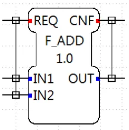
It is also possible to associate input events with input data ports, as shown in Figure 2.2. This is achieved by using the WITH qualifier [1]. There are two types of association. The first type defines an association between one input event port with one or more data input ports, while the second one defines an association between one output event port with one or more data output ports [1]. The first type of association is used in order to retrieve information regarding the set of input data ports that will be read together with the input event port that are associated with [1]. The second type of association defines the set of output data ports that will be updated together with the output event port. Figure 2.2 illustrates a Function Block with one input event called REQ and two input variables on the left side, IN1 and IN2. In addition, it produces one output event and one output variable, namely CNF and OUT respectively, which are shown in the right side and are sent to the following Function Blocks that are connected with it. In the center of the BFB we state its name F_ADD. Finally, we also define the version of the BFB, which is in our example 1.0. The version is used in order for the engineers to recognize how many updates have been applied to the specific BFB.

(11)

10

2.3.2 Service Interface Function Blocks

According to Lednicki [1], Service interface function blocks are used as interfaces of external services. The IEC 61499 standard does not fully documents SIFBs but they may conclude a sequence diagram in order to express the behavior of the SIFB [1]. SIFBs provide same FB interface as other FB types. The main difference is that the execution of an SIFB can start independently to arrival of input events.

2.3.3 Composite Function Block

A CFB, as the name implies, is built by composing BFBs, SIFBs and other CFBs. Similarly to the BFBs, a CFB has a set of input variables and a set of output events. In addition, it provides a set of event outputs and a set of event variables. Furthermore, the variables and the events may be associated with each other [6] similarly to BFBs.

The Function Blocks that are used internally in the CFB are connected with each other in order to provide its functionality. Therefore, by using CFBs it is possible to represent the complex software functionality.

2.3.4 Function Block Network

A function block network consists of several FBs, CFBs and SIFBs. The elements of a FBN are connected with each other with the ports of these elements [1]. In principle, FBN is used in order to express the functionality of a control system. It can be also used in order describe the structure of a CFB. Figure 2.3 illustrates a simple FBN.

(12)

11

2.4. The 4DIAC initiative

Over the recent years only few tools are created in order for an engineer to develop an application based on IEC 61499. One of the main reasons for this is that the standard does not clearly define how the FBs will be executed [4]. Some of the most well-known and widely used tools are: 4DIAC [13], Function Block Development Kit [10], nxtStudio [11] and ISaGRAF [12].

This thesis report will focus on the 4DIAC-IDE tool. The main purpose of this tool is to give an opportunity to the developers to use an open-source framework that supports completely the IEC 61499 standard and provides a big extent automation and control environment. It is developed by PROFACTOR GmbH and provides an editor for ECLIPSE that can be used in order to create FBs, CFBs and SIFBs[13]. The standard is based on Graphical Editing Framework, which is used in order to develop graphical user interfaces.

There are two main projects which are developed by 4DIAC initiative [12]. The first one is the 4DIAC-RTE/FORTE which is a runtime environment, implemented in C++, complied with IEC 61499 standard and is used for developing simple control automated systems [12]. It supports development of the basic elements described in the standard, namely FBs, CFBs and FBNs. The second project is the 4DIAC-IDE which can be seen as an extension of 4DIAC-RTE/FORTE since it is an extensive framework that is used for developing large distributed automation applications [12].

2.5. State Of The Art

Over the recent years, there has been an extensive research on several perspectives of the IEC 61499 standard. In [14] Thramboulidis discuss the vagueness regarding execution semantics of an ECC. The problem stems from the fact that the IEC 61499 standard does not clarify the order of the execution of the FBs in cases where there is more than one FBs ready to be executed. As result of this, manufacturers of distributed automated systems follow different approaches regarding the execution of the application. In [15] Čengić et al. showed how the same application may have different behavior depending on the platform that is executed. Sünder et al. [16] investigated this matter even further in terms of discussing how the event ports that are contained in a FBN are scheduled.

In addition, several researchers investigate how we can have a plain transition from PLC’s to the 61499 standard. Wegner et al. [18] suggested a transformation of a PLC application to an application that will be complied with 61499 standard, while Gerber et al. [19] suggested a manual migration. Furthermore in [2] Zoitl presents how we can use the programming languages defined in IEC 61131-3 standard in IEC 61499 FBs in order to achieve a certain level of harmonization between the two standards.

(13)

12

3. Method

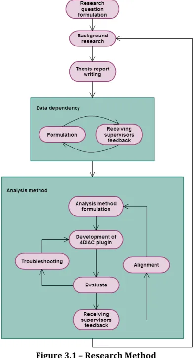
The research method that was used during this thesis is illustrated in Figure 3.1. In the beginning the research questions related to the thesis were stated (problem formulation). Then the necessary background research was conducted. During this activity, we gathered all the information from previous topics that are related to this thesis. The purpose of the thesis is to investigate how we can analyze the dependency between input and output data ports. In order to do that, we developed and formulated the theory behind the analysis method. In addition, a research for gathering state of the art and related work was conducted. Based on this information an analysis method was formulated. This analysis method answered the questions that were previously formulated.

Afterwards, we analyzed and evaluated our results by implementing a plug-in for the 4DIAC-IDE tool which validated our theory. Finally, all the results of this research were discussed and presented in the thesis report.

(14)

13

4. Formal definition of IEC 61499

In order to continue this report with the description of data dependency analysis, first we must address needed definitions of the used IEC 61499 elements. This section presents these definitions. Parts of the definitions presented in this report are based on the work of Čengić and Åkesson [7] and Lednicki [1]. Definitions that vary from the ones defined in the mentioned paper and Ph.D. dissertation are formed based on the IEC 61499 standard definition [3]. Elements that are not significant for this work, such as event ports and connections between them, are disregarded.

Definition 1. A function block interface is defined as: Function block interface:

𝐼 = 〈𝐷𝑖, 𝐷𝑜〉, where

𝐷𝑖 is a set {𝑑𝑖0, … , 𝑑𝑖|𝐷𝑖|} of data inputs;

𝐷_𝑜 is a set {𝑑_𝑜0, … , 𝑑_𝑜|𝐷_𝑜|} of data outputs.

Definition 2. A basic function block and its subcomponents are defined as: Basic function block:

𝑏𝐹𝐵 = 〈𝐼, 𝐸𝐶𝐶, 𝐼𝑛𝑡𝑉𝑎𝑟𝑠〉, where

𝐼 is a function block interface;

𝐸𝐶𝐶 is an execution control chart (ECC);

𝐼𝑛𝑡𝑉𝑎𝑟𝑠 is a set {𝐼𝑛𝑡𝑉𝑎𝑟₀, … , 𝐼𝑛𝑡𝑉𝑎𝑟_{|𝐼𝑛𝑡𝑉𝑎𝑟𝑠|}} of internal variables. Execution control chart (ECC):

𝐸𝐶𝐶 = 〈𝑆, 𝑇, 𝐴〉, where

𝑆 is a set {𝑠₀, … , 𝑠_|𝑆|} of ECC states; 𝑇 is a set {𝑡0, … , 𝑡|𝑇|} of ECC transitions.

𝐴 is a set of algorithm functions. ECC state:

𝑠 = 〈𝑠𝑎1, … , 𝑠𝑎|𝑆|〉, where

𝑠𝑎_𝑖 is an ECC state action. ECC state action:

𝑠𝑎 = {𝑎0, … , 𝑎|𝑠𝑎|} , where

(15)

14 ECC transition:

𝑡 = 〈𝑠_𝑠, 𝑠_𝑑, 𝑔〉, where

𝑠𝑠 is the source state, 𝑠𝑠𝜖𝑆;

𝑠𝑑 is the destination state, 𝑠𝑑𝜖𝑆;

𝑔 the guard of the transition. Guard of transition:

𝑔 = 〈𝐺𝐼𝑛𝑡𝑉𝑎𝑟𝑠, 𝐺𝐷_𝑖〉, where

𝐺𝐼𝑛𝑡𝑉𝑎𝑟𝑠 a set of internal variables used in the guard, where 𝐺𝐼𝑛𝑡𝑉𝑎𝑟𝑠 ⊆ 𝐼𝑛𝑡𝑉𝑎𝑟𝑠;

𝐺𝐷_𝑖 a set of data inputs used in the guard, where 𝐺𝐷_𝑖 ⊆ 𝐷_𝑖. Definition 3. A composite function block and its elements are defined as: Composite function block:

𝑐𝐹𝐵 = 〈𝐼, 𝐹𝐵𝑛〉, where

𝐼 is a function block interface.

𝐹𝐵𝑛 is the internal function block network. Function block network:

𝐹𝐵𝑛 = 〈𝐹, 𝐶〉, where

F is a set of function blocks, each of which is either 𝑏𝐹𝐵, 𝑠𝑖𝐹𝐵 or 𝑐𝐹𝐵;

C a set of connections between data ports, where 𝐶 = {𝑐0, … , 𝑐|𝑐|}

Connection:

𝑐 = 〈𝑑_𝑠, 𝑑_𝑑〉, where

𝑑_𝑠 is the data port used as the source of the connection; 𝑑_𝑑 is the data port used as the connection target.

(16)

15

5. Results

Now that we have described the needed IEC 61499 elements that we will use in the analysis, we can present the actual analysis method. This chapter will outline data dependency analysis method on three levels. First one is the algorithm level, while second and third level present basic and composite function blocks analysis respectively. In addition to the detailed algorithms explanations, we will present a 4DIAC plug-in which implements the previously mentioned analysis method. This implementation is used to evaluate the analysis method.

To answer RQ1, on which ways can output data be dependent on input data based on the IEC 61499 standard, we distinguish eight different types of data dependency:

1. An output data depends on input data on the algorithm level.

2. An output data depends on internal variable on the algorithm level. 3. An output data depends on data input on FB level.

4. An output data depends on internal variable on FB level.

5. An internal variable depends on data input on the algorithm level.

6. An internal variable depends on internal variable on the algorithm level. 7. An internal variable depends on data input on FB level.

8. An internal variable depends on internal variable on FB level.

Dependency types 1 to 4 are considered to be direct data dependency, while dependency types 5 to 8 are considered to be indirect data dependency. In the following sections all these types of dependency will be thoroughly analyzed with the use of examples.

5.1 Data dependency analysis in the algorithm level

The lowest level of the IEC 61499 model hierarchy consists of algorithms that are implemented by code and not defined by models. Determining the data dependency based on this code is outside the scope of this thesis report. We assume that the analysis of the code is previously done and that the data dependency information that is retrieved by the algorithms is already available.

Data dependency types 1, 2, 5 and 6 fall into this category.

5.1.1 Data Dependency Type 1

In this case the result of the calculation for each data output is related to one or more data inputs. This means that in order for the algorithm to produce the value of the data output, it is necessary to know the values of data inputs. Consequently, the data output depends on these data inputs. The algorithm REQ, shown in Listing 1, is part of a Function Block named F_BAND_B, that has two data input ports X and B and one data output port OUT. Having a closer look at the statements of this algorithm, we notice that the input is used to calculate the output (line 6). In addition, we notice that the input is used in control flow statements of the program, for example “if… else” blocks. In these statements, updates to an output are influenced by the value of input ports (lines 1 and 2).

(17)

16 1 IFX < BTHEN 2 OUT := 0; 3 ELSIFX > 255-BTHEN 4 OUT := 255; 5 ELSE 6 OUT := X; 7 END_IF;

In this case the result of the calculation of the data output is related to one or more internal variables that are used in the algorithm. This is visible in listing 2, which presents algorithm REQ of a basic function block named FB_INTEGRATE version 0.0 that has three data input ports X, K and reset and one data output port, Y_OUT. This BFB has additional four internal variables X_last, last, tx and Y_intern. There are two states in the ECC for this BFB, named INIT and REQ. For the purpose of this example we will investigate the algorithm of the state REQ.

1 IFresetTHEN

2 Y_intern := 0.0;

3 ELSE

4 tx := T_PLC_MS();

5 Y_intern := (X + X_last) * 0.5E-3 * DWORD_TO_REAL(tx - last) * K + Y_intern;

6 X_last := X;

7 last := tx; 8 END_IF;

9 Y_OUT := Y_intern;

As we can see, in line 9 in order to calculate the data output Y_OUT we need to know the value of the internal variable Y_intern. This is a typical example of a data dependency where an output data depends on an internal variable

In this type of data dependency an internal variable depends on a data input. Then the internal variable is used to calculate a data output. Therefore, the data output depends on the internal variable. In addition, the internal variable depends on the data input. As a result of this, we conclude that the data output depends on the data input. This is visible in the example of the previous section. Internal variable Y_intern depends on data input

X, since, in order to calculate it, we need to know the value of X (line 5). Furthermore,

data output Y_OUT depends on internal variable Y_intern (line 9). As a result of these dependencies, we conclude that there is an indirect dependency between data output

Y_OUT and data input X.

Listing 1 – REQ Algorithm

(18)

17

In this type of data dependency, an internal variable depends on another internal variable. Then the first internal variable is used in order to calculate a data output and because of the data dependency between the two internal variables, we conclude that the data output depends in the second internal variable as well. This is clearly visible in the example of algorithm we presented in section 5.1.2. In line 5 we notice that internal variable Y_intern depends on internal variables X_last, last and tx. In addition, internal variable Y_intern is used in order to calculate the data output Y_OUT. Thus, data output

Y_OUT depends also on the internal variables X_last, last and tx.

As we mentioned in the beginning of section 5.1, we will use as an input the data dependency analysis on the algorithm level in our analysis methods, in order to conclude for data dependencies between data inputs and data outputs in the BFB and CFB level.

5.2 Data dependency analysis in the FB level

In this section we will analyze data dependency types 3, 4, 7 and 8. These types of dependency occur in the FB level, which means we will have to analyze the ECC of the Function Block in order to conclude for data dependencies.

5.2.1 Data Dependency type 3

According to data dependency type 3, a data output depends on a data input on the FB level. This occurs when one or more data inputs are used in the guards of the transitions between the various states of the ECC. As a result of this, the data outputs that are used in the destination states of the transitions, where the data inputs are used, depend on these data inputs. This is visible in the following example.

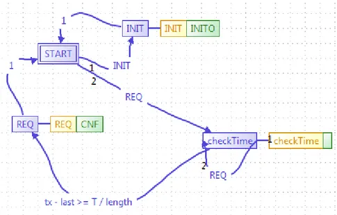
Figure 5.1 represents the ECC of the FB_FT_TN16 Function Block. This function block has two data inputs, namely IN and T and one data output OUT. In addition, it uses the internal variables length, X, cnt, last and tx. As we can see from the figure in the

(19)

18

transition from checkTime state to REQ state we use as a guard a comparison condition. If this condition holds, then we can go to the destination state (REQ). In this condition we use the data input T. As a result of this, all the data outputs that are used in the algorithm of the destination state will be dependent on the data input T.

Based on this type of data dependency, a data output depends on one or more internal variables. In order for this to happen, these internal variables should be used in the guards of the transitions. Then we conclude that all the data outputs that are used in the destinations state of the transition will be dependent on these internal variables. This is clearly visible in the example that we mentioned in the previous section. The guard of the transition from checkTime state to REQ state uses the internal variables x, last and

length. Therefore, we conclude that all the data outputs that are used in the algorithm of

the destination state (REQ) will be dependent on these internal variables.

This type of dependency is related to the internal variables that are used in algorithms when they depend on data inputs, which are used in the guards of the transitions between the states. In order for this to happen, one or more data inputs need to be used in the guard of a transition, and the algorithm(s) of the destination state need to use one or more internal variables. Then one or more data outputs depend on these internal variables. Therefore, we conclude that the data outputs of the destination state are dependent on the data inputs that were used in the guard. The following listing presents the code of the algorithm REQ of the previous example.

1 IF cnt = length - 1THEN 2 cnt := 0; 3 ELSE 4 cnt := cnt + 1; 5 END_IF 6 OUT := X[cnt]; 7 X[cnt] := IN; 8 last := tx;

In this listing we notice that the data output OUT depends on the internal variable cnt (line 6). In addition the internal variable cnt depends on the data input T that is used in the guard of the transition. Consequently, we say that the data output OUT depends on the internal variable cnt.

This last type of data dependency is related to internal variables that are used in an algorithm of a state and internal variables that are used in the guard of the transition, which reaches the state where the algorithm belongs to. In addition, we assume that a data output depends on one internal variable that is used in the algorithm. If this internal variable depends on the internal variables of the guards then we say that the data output depends on the internal variables of the guards as well. This is visible in the

(20)

19

Figure 5.2 – (a) BFB interface (b) ECC BFB analysis example

example that we presented in the section 5.2.1 and 5.2.2. There, the data output OUT depends on the internal variable cnt. But the internal variable cnt depends on the internal variables tx, last and length that are used in the transition of the guard. Therefore we conclude that the data output OUT depends on the internal variables tx,

last and length.

In order to answer RQ2 on which method can we use for calculating data dependency, two analysis methods were formulated. The first one investigates dependency on BFBs and is presented in the Section 5.2.1. Respectively, Section 5.2.2 presents CFBs dependency analysis method.

5.3 Basic Function Block Dependency Analysis Method

The Basic Function Block Dependency Analysis Method is used in order to determine the data dependencies between data inputs and data outputs. It consists of 4 algorithms, namely do_Analysis, UpdateMatrix, coverIndirectDependency_1 and coverIndirectDependency_2. We start the basic function block analysis by reading all data input and output ports from the interface. To explicitly show dependencies between input and output data ports for IEC 61499 function blocks, we introduced a dependency matrix. The matrix consists of rows representing data inputs and columns representing data outputs. A cell represents an ordered pair of data input and data output. If there is a dependency for that ordered pair, then their cell is set to a value 1, otherwise 0. Afterwards, we go through each algorithm of a state, where we read the existing information regarding which data output port is dependent on which data input port. This is achieved with the UpdateMatrix algorithm. Once the dependency among a pair of data output and data input is found, their cell value in dependency matrix is changed from 0 to 1. The coverIndirectDependency_1 and coverIndirectDependency_2 are two algorithms that are called inside the UpdateMatrix algorithm and are used in order to cover the several types of data dependencies that we defined by answering the RQ1. We will present an example that will be used in order to explain how the algorithms work.

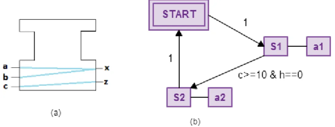
In Figure 5.2 (a) we present the interface of the BFB. This FB has three data inputs, namely a, b and c, and two data outputs, namely x and z. In addition the FB has three internal variables h, i and g. In Figure 5.2 (b) we show the ECC of this FB. We notice that this ECC has two states S1 and S2 with one algorithm in each state a1 and a2 respectively. The code of each algorithm is presented in listing 4 and 5.

(21)

20 1 x := a+1; 2 x := i; 3 c := 10; 4 h := 0; 5 i := b+1; 6 i := g+10;

We start the analysis method by iterating over the transitions of the ECC. Therefore we start with the first transition from state Start to state s1. This transition has no guard, and thus we have no data inputs or internal variables to take into account for the destination state. Once we found the destination state we iterate over the algorithms of it. In this case we have only one algorithm called a1. We retrieve the information regarding data dependencies between data inputs and outputs in the algorithm level. For algorithm a1 we notice that there is a dependency between data output x and data input a. Thus, in the dependency Matrix we update the respective cell from 0 to 1. In addition, we update the cells of the dependency Matrix that indicate dependency between internal variables.

It is important to mention at this point that the internal variables are included in the dependency matrix during the BFB analysis. Thus, we add next to the data inputs and the data outputs the internal variables of the algorithm. This is done in order to save also dependencies between data outputs and internal variables. The result of the BFB analysis though will not contain the internal variables, since it should be on the level of BFB interface and contain only data inputs and data outputs that are visible on the interface level. Thus we hide the complexities of the internal BFB structures.

In addition we check if there is a dependency between internal variables and data outputs. In algorithm a1 we notice that there is a dependency between data output x and internal variable i. Thus we will update the respective cell in the dependency matrix from 0 to 1. The next step in the analysis method is to transform data dependencies type 6 to 2. This means that we will check for each data output if it depends on internal variable(s) that depend(s) on other internal variable(s). We notice that internal variable

i depends on internal variable g. Thus we conclude that data output x depends on

internal variables g as well. At this point the dependency Matrix is as shown in step 1 in figure 5.3.

1 z := 3;

(22)

21

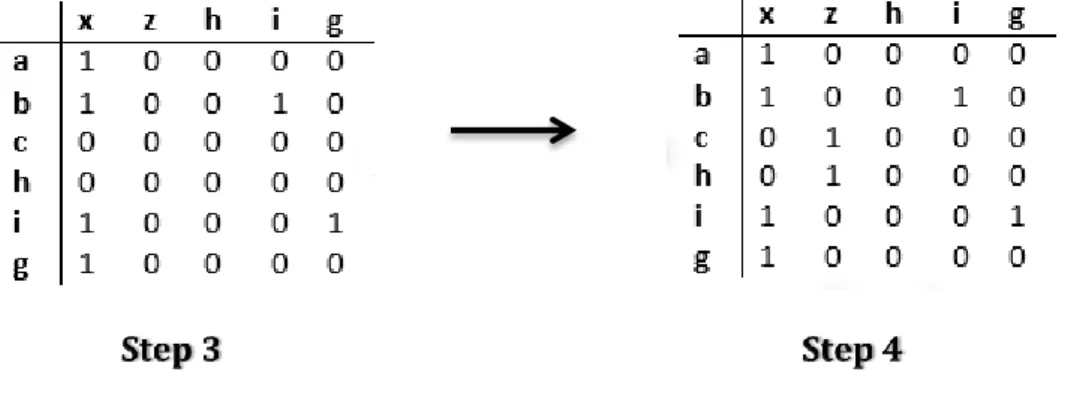
The next step in the algorithm analysis is to transform data dependency type 5 to type 1. This means that we have data outputs that depend on internal variables, which depend on data inputs. In our algorithm we notice that data output x depends on internal variable i which depends on data input b. Therefore there is a dependency between data output x and data input b. This is shown in step 2 from figure 5.4. Once we completed the dependency analysis for algorithm a1 we go to the next transition. This transition uses in its guard data input c and internal variable h. Therefore the data outputs, which are used in the algorithms of the destination state, will be dependent on this data input and internal variable. In our case there is only one algorithm that will be executed, that is s2. This algorithm contains only one data output, namely z. Therefore this data output will be dependent on data input x and internal variable h, as shown in step 3 of figure 5.4 below.

doAnalysis Algorithm

Algorithm 1 is used in order to iterate over all the transitions of the ECC. In line 1 we define the basic function block as a set of data inputs and data outputs, that are retrieved by the interface of the function block, an ECC, a set of transitions of the ECC and a set of Algorithms in the ECC. In line 3 we iterate over the transitions of the ECC. For each transition we define a set of internal variables and a set of data inputs that are used in the guard of the transition (lines 4 and 5). Then, for each of the algorithms of each of the state actions of the destination state we call the algorithm 2 named updateMatrix.

Figure 5.3 – Stages of the Dependency Matrix

(23)

22 Algorithm 1 doAnalysis()

1: 〈〈𝐷𝑖, 𝐷𝑜〉, 〈𝑆, 𝑇, 𝐴〉, 𝐼𝑛𝑡𝑉𝑎𝑟𝑠〉 ← 𝑏𝐹𝐵

2: Let 𝑀𝑏𝐹𝐵 be the zero − filled dependency matrix of bFB 3: for each 𝑡 ∈ 𝑇 do

4: Let 𝑔𝑢𝑎𝑟𝑑_𝑣𝑎𝑟𝑠 be a set of internal variables used in the guard of t 5: Let 𝑔𝑢𝑎𝑟𝑑_𝑖𝑛𝑝𝑢𝑡𝑠 be set of data inputs used in the guard of 𝑡 6: Let 𝑑𝑒𝑠𝑡_𝑠𝑡𝑎𝑡𝑒 be the destination state of 𝑡

7: for each 𝑠𝑎 ∈ 𝑑𝑒𝑠𝑡_𝑠𝑡𝑎𝑡𝑒 do 8: for each 𝑎 ∈ 𝑠𝑎 do

9: 𝑢𝑝𝑑𝑎𝑡𝑒𝑀𝑎𝑡𝑟𝑖𝑥(𝑎, 𝑔𝑢𝑎𝑟𝑑_𝑣𝑎𝑟𝑠, 𝑔𝑢𝑎𝑟𝑑_𝑖𝑛𝑝𝑢𝑡𝑠)

10: end for each

11: end for each 12: end for each

updateMatrix Algorithm

This algorithm is used in order to update the Matrix that represents the dependency between data inputs and data outputs. In lines 1 and 2 of the algorithm we define a set of data outputs and internal variables that are used in the algorithm 𝛼. In lines 3 to 10 we iterate over the internal variables of the algorithm. In lines 4 and 5 we retrieve the information for dependency between the internal variable and the data inputs and other internal variables that are used in the algorithm. Based on this information, we update the matrix in case there is a dependency between the internal variable and the data input or other internal variable.

In lines 11 to 22 we iterate over the data outputs of the algorithm 𝛼. In this loop we will update the dependency Matrix when we detect a dependency between data input and data output, or internal variable and data output, or an internal variable or data input used in the guard and the data output. In lines 12 and 13 we retrieve the information for dependency between the data output and the data inputs and internal variables that are used in the algorithm. Based on this information in the two loops of lines 14-15 and 16-17 we update the dependency matrix. In lines 18 to 21 we update the matrix in order to save the dependency between the data output and the data inputs and internal variables that are used in the guard. Once we iterate over this procedure for every data output of the algorithm then we iterate over a loop by calling the algorithm coverIndirectDepedency_1. This is done in order to transform data dependencies types 6 to data dependency type 2. When this is done, we call the algorithm coverIndirectDependency_2 in order to transform data dependencies types 2 and 5 to data dependency type 1.

Algorithm 2 UpdateMatrix(𝑎, 𝑔𝑢𝑎𝑟𝑑_𝑣𝑎𝑟𝑠, 𝑔𝑢𝑎𝑟𝑑_𝑖𝑛𝑝𝑢𝑡𝑠) 1: Let 𝑑𝑎𝑡𝑎_𝑜𝑢𝑡𝑝𝑢𝑡𝑠 be a set of data outputs of 𝛼

2: Let 𝑖𝑛𝑡𝑒𝑟𝑛𝑎𝑙_𝑣𝑎𝑟𝑖𝑎𝑏𝑙𝑒𝑠 be a set of internal variables of 𝛼 3: for each 𝑖𝑛𝑡𝑒𝑟𝑛𝑎𝑙_𝑣𝑎𝑟𝑖𝑎𝑏𝑙𝑒 in 𝑖𝑛𝑡𝑒𝑟𝑛𝑎𝑙_𝑣𝑎𝑟𝑖𝑎𝑏𝑙𝑒𝑠 do

4: Let 𝑑𝑒𝑝_𝑑𝑎𝑡𝑎_𝑖𝑛𝑝𝑢𝑡𝑠 be a subset of data inputs of 𝛼 that 𝑖𝑛𝑡𝑒𝑟𝑛𝑎𝑙_𝑣𝑎𝑟𝑖𝑎𝑏𝑙𝑒 depends on

5: Let 𝑑𝑒𝑝_𝑖𝑛𝑡𝑒𝑟𝑛𝑎𝑙_𝑣𝑎𝑟𝑖𝑎𝑏𝑙𝑒𝑠 be a set of internal variables of 𝛼 that 𝑖𝑛𝑡𝑒𝑟𝑛𝑎𝑙_𝑣𝑎𝑟𝑖𝑎𝑏𝑙𝑒 depends on

6: for each 𝑖𝑛𝑡_𝑣𝑎𝑟 in 𝑑𝑒𝑝_𝑖𝑛𝑡𝑒𝑟𝑛𝑎𝑙_𝑣𝑎𝑟𝑖𝑎𝑏𝑙𝑒𝑠 do 7: 𝑀𝑏𝐹𝐵 [𝑖𝑛𝑡𝑒𝑟𝑛𝑎𝑙_𝑣𝑎𝑟𝑖𝑎𝑏𝑙𝑒, 𝑖𝑛𝑡_𝑣𝑎𝑟] = 1

(24)

23

8: for each 𝑑𝑎𝑡𝑎_𝑖𝑛𝑝𝑢𝑡 in 𝑑𝑒𝑝_𝑑𝑎𝑡𝑎_𝑖𝑛𝑝𝑢𝑡𝑠 do 9: 𝑀𝑏𝐹𝐵 [𝑖𝑛𝑡𝑒𝑟𝑛𝑎𝑙_𝑣𝑎𝑟𝑖𝑎𝑏𝑙𝑒, 𝑑𝑎𝑡𝑎_𝑖𝑛𝑝𝑢𝑡] = 1 10: end for each

11: for each 𝑑𝑎𝑡𝑎_𝑜𝑢𝑡𝑝𝑢𝑡 in 𝑑𝑎𝑡𝑎_𝑜𝑢𝑡𝑝𝑢𝑡𝑠 do

12: Let 𝑑𝑒𝑝_𝑑_𝑖𝑛𝑝𝑢𝑡𝑠 be a subset of data inputs of 𝛼 that 𝑑𝑎𝑡𝑎_𝑜𝑢𝑡𝑝𝑢𝑡 depends on

13: Let 𝑑𝑒𝑝_𝑖𝑛𝑡_𝑣𝑎𝑟𝑠 be a set of internal variables of 𝛼 that 𝑑𝑎𝑡𝑎_𝑜𝑢𝑡𝑝𝑢𝑡 depends on 14: for each 𝑖𝑛𝑡𝑒𝑟𝑛𝑎𝑙_𝑣𝑎𝑟𝑖𝑎𝑏𝑙𝑒 in 𝑑𝑒𝑝_𝑖𝑛𝑡_𝑣𝑎𝑟𝑠 do 15: 𝑀𝑏𝐹𝐵 [𝑑𝑎𝑡𝑎_𝑜𝑢𝑡𝑝𝑢𝑡, 𝑖𝑛𝑡𝑒𝑟𝑛𝑎𝑙_𝑣𝑎𝑟𝑖𝑎𝑏𝑙𝑒] = 1 16: for each 𝑑𝑎𝑡𝑎_𝑖𝑛𝑝𝑢𝑡 in 𝑑𝑒𝑝_𝑑_𝑖𝑛𝑝𝑢𝑡𝑠 do 17: 𝑀𝑏𝐹𝐵 [𝑑𝑎𝑡𝑎_𝑜𝑢𝑡𝑝𝑢𝑡, 𝑑𝑎𝑡𝑎_𝑖𝑛𝑝𝑢𝑡] = 1 18: for each 𝑔𝑢𝑎𝑟𝑑_𝑣𝑎𝑟 in 𝑔𝑢𝑎𝑟𝑑_𝑣𝑎𝑟𝑠 do 19: 𝑀𝑏𝐹𝐵 [𝑑𝑎𝑡𝑎_𝑜𝑢𝑡𝑝𝑢𝑡, 𝑔𝑢𝑎𝑟𝑑_𝑣𝑎𝑟] = 1 20: for each 𝑔𝑢𝑎𝑟𝑑_𝑖𝑛𝑝𝑢𝑡 in 𝑔𝑢𝑎𝑟𝑑_𝑖𝑛𝑝𝑢𝑡𝑠 do 21: 𝑀𝑏𝐹𝐵 [𝑑𝑎𝑡𝑎_𝑜𝑢𝑡𝑝𝑢𝑡, 𝑔𝑢𝑎𝑟𝑑_𝑖𝑛𝑝𝑢𝑡] = 1 22: end for each

23: checker =1;

24: while checker !=0

25: checker = coverIndirectDependency_1() 26: coverIndirectDependency_2()

coverIndirectDependency_1 Algorithm

As we mentioned before, Algorithm 3 is used in order to transform data dependency type 6 to data dependency type 2. We iterate the procedure of the algorithm for each of the data outputs of the Function Block (lines 2 to 14). For each of the data outputs we check if there is dependency between this data output and all the internal variables (line 4). Then for this internal variable, we check in line 6, whether there is a data dependency with another internal variable, which is actually the data dependency type 6. If this condition holds then we say that there is a data dependency between the data output and the internal variable. Therefore we transformed data dependency type 6 to data dependency type 2.

Algorithm 3 coverIndirectDependency_1() 1: checker =0;

2: for each 𝑑𝑎𝑡𝑎_𝑜𝑢𝑡𝑝𝑢𝑡 in the 𝑀𝑏𝐹𝐵 do

3: for each 𝑖𝑛𝑡𝑒𝑟𝑛𝑎𝑙_𝑣𝑎𝑟𝑖𝑎𝑏𝑙𝑒 in the 𝑀𝑏𝐹𝐵 do

4: if 𝑀𝑏𝐹𝐵 [𝑑𝑎𝑡𝑎_𝑜𝑢𝑡𝑝𝑢𝑡, 𝑖𝑛𝑡𝑒𝑟𝑛𝑎𝑙_𝑣𝑎𝑟𝑖𝑎𝑏𝑙𝑒] == 1

5: for each 𝐼𝑛𝑡𝑉𝑎𝑟 in the 𝑀𝑏𝐹𝐵 do

6: if 𝑀𝑏𝐹𝐵 [𝑖𝑛𝑡𝑒𝑟𝑛𝑎𝑙_𝑣𝑎𝑟𝑖𝑎𝑏𝑙𝑒, 𝐼𝑛𝑡𝑉𝑎𝑟] == 1 7: if 𝑀𝑏𝐹𝐵 [𝑑𝑎𝑡𝑎_𝑜𝑢𝑡𝑝𝑢𝑡, 𝐼𝑛𝑡𝑉𝑎𝑟] == 0 8: 𝑀𝑏𝐹𝐵 [𝑑𝑎𝑡𝑎_𝑜𝑢𝑡𝑝𝑢𝑡, 𝐼𝑛𝑡𝑉𝑎𝑟] = 1 9: checker = 1; 10: end if 11: end if

13: end if

14: end for each 15: return checker

(25)

24

The variable checker is used in order to iterate over the loop of line 5 as many times as it is needed so that we can cover the case where there is a dependency between more than two internal variables.

CoverIndirectDependency_2 Algorithm

The next step is to call algorithm 4. In terms of structure, this algorithm is similar to the previous one. The purpose of it is to transform data dependency type 5 to type 1. This is achieved by iterating over every data output in lines 2 to 12. For each of the data outputs and for each of the internal variables we check if there is data dependency between them (line 4). If yes, then we check if there is any data dependency between this internal variable and the data inputs. This is achieved in line 6. If there is data dependency, then we update the matrix so that we define a data dependency between the data input and the data output (line 7). Thus, we transformed data dependency type 5 to data dependency type 1.

Algorithm 4 coverIndirectDependency_2() 2: for each 𝑑𝑎𝑡𝑎_𝑜𝑢𝑡𝑝𝑢𝑡 in the 𝑀𝑏𝐹𝐵 do

3: for each 𝑖𝑛𝑡𝑒𝑟𝑛𝑎𝑙_𝑣𝑎𝑟𝑖𝑎𝑏𝑙𝑒 in the 𝑀𝑏𝐹𝐵 do

4: if 𝑀𝑏𝐹𝐵 [𝑑𝑎𝑡𝑎_𝑜𝑢𝑡𝑝𝑢𝑡, 𝑖𝑛𝑡𝑒𝑟𝑛𝑎𝑙_𝑣𝑎𝑟𝑖𝑎𝑏𝑙𝑒] == 1

5: for each 𝑑𝑎𝑡𝑎_𝑖𝑛𝑝𝑢𝑡 in the 𝑀𝑏𝐹𝐵 do

6: if 𝑀𝑏𝐹𝐵 [𝑖𝑛𝑡𝑒𝑟𝑛𝑎𝑙_𝑣𝑎𝑟𝑖𝑎𝑏𝑙𝑒, 𝑑𝑎𝑡𝑎_𝑖𝑛𝑝𝑢𝑡] == 1

7: 𝑀𝑏𝐹𝐵 [𝑑𝑎𝑡𝑎_𝑜𝑢𝑡𝑝𝑢𝑡, 𝑑𝑎𝑡𝑎_𝑖𝑛𝑝𝑢𝑡] = 1

9: end if

11: end if

12: end for each 13: end for each

The analysis method that we defined in this section covers the data dependencies types 1 to 6. A limitation of the suggested solution, which would be interested to investigate even further, is to extend it in order to cover data dependencies types 7 and 8. That is, data dependencies that derive from the fact that an internal variable is dependent on a data input or on another internal variable that are used in the guards of the transitions of the ECC. Another aspect of the proposed analysis method that we should mention is that it does not cover the case where the ECC is cyclic.

In our solution we consider only the direct destination state to be dependent on data inputs and internal variables used in the guards of the transitions. But there is a case, where from a transition T1 with a data input in the guard, we go to state S1 and from state S1, we go to state S2 without using a guard in the transition. This means that the data outputs of state S2 are also dependent on the data input that is used in the transition T1. This case can be generalized when the ECC is cyclic. Therefore the suggested analysis method takes into account only direct dependencies from data inputs and internal variables used in the transitions to the data outputs used in the algorithms of the destination state.

(26)

25

5.4 Composite Function Block Dependency Analysis Method

For the dependency analysis method of a CFB we have created two algorithms. First algorithm starts the CFB analysis using the information defined on the CFB interface level, while the second one performs recursive network analysis. The reason that we use two algorithms is that we need to read only once the interface of the CFB in order to find data input ports. After reading the interface, the dependency matrix is initialized and all its values are set to 0. The function doDependencyAnalysis is called for each data input port. This algorithm goes through each and every connection of the data input port to find the destination data input port. If the destination data input port is one of the data output ports of the CFB then the dependency matrix is updated. If this is not the case, for each data output which depends on the destination data input port we call recursively doDependencyAnalysis algorithm.

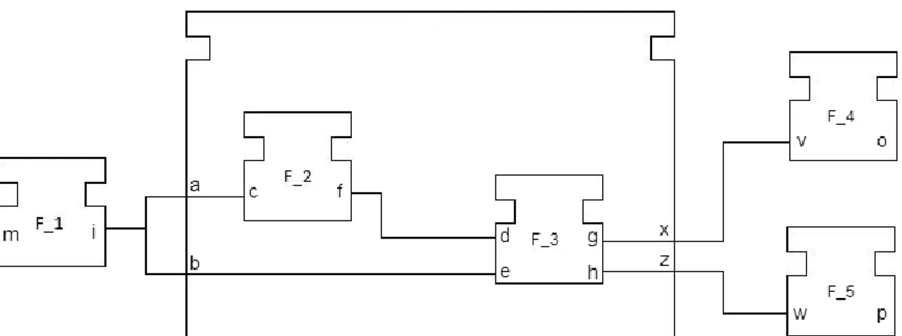
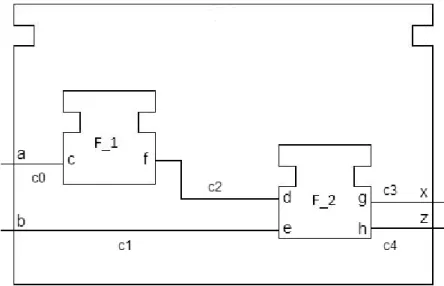
Figure 5.5 captures a composite function block that we will use in order to explain data dependency analysis on them. This CFB has two data inputs a and b, and two data outputs x and z. In addition, this CFB consists of two BFBs. First BFB, named F_1, has one data input c and one data output f. Second BFB, named F_2, contains two data inputs d and e, and two data outputs g and h.

In order to find dependencies in CFB we start by searching all the connections for each data input. For this example, we begin with the data input a and we find that there is one connection c0 to BFB F_1, and its data input c. When visiting BFBs that are inside of a CFB we retrieve also their dependency matrix.

Figure 5.5 – CFB analysis example

(27)

26

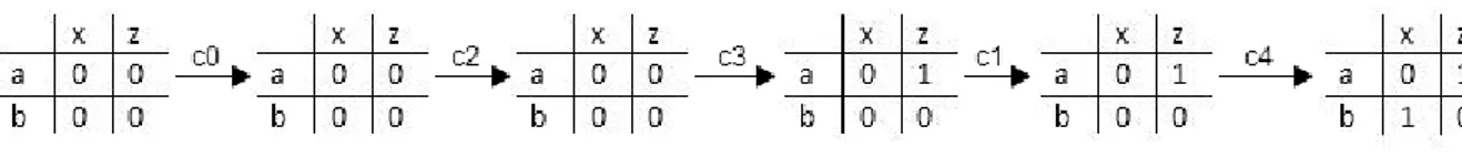
With this information we know that there is a data dependency between data output f and data input c of F_1. Next, we search for connections of a data port f. This is done by calling recursively doDependencyAnalysis function. Next connection, named c2 leads us to the BFB F_2 and its data input port d. Dependency matrix of F_2 tells us that data output port h is dependent on data input port d. Now we follow the connection c4 from the data output port d to data output port of a CFB z. Here we have found the first data dependency on the level of CFB. The cell in dependency matrix that corresponds to data output z and data input a is changed from 0 to 1. Since we have come to the end of connections for the data output z, we come back to the beginning and start looking into data input port b. We are following the same procedure which leads us to BFB F_2 and data input e, by going through connection c1. Dependency matrix of BFB F_2 tell us that within it there is a dependency between data output port g and data input port e. Next we search for connections deriving from data output g. This connection, called c3, connects CFB data output port x with BFB F_2 data output port g. Finally, we have found the second data dependency for this CFB. This dependency is between data output port x and data input port b. Having in mind that we have visited all connections all that is left to do is to update the dependency matrix.

Figure 5.7 presents all the stages that dependency matrix is going through. The dependency matrix is updated every time we reach a data output of the CFB.

The CFB Dependency Analysis Algorithm

Algorithm 5 defines the dependency analysis of a composite function block. The for loop starting on the line 3 is used to iterate over all data input ports. For each of the data input ports we will call the function doDependencyAnalysis. The doDependencyAnalysis function performs a recursive analysis starting from the port, and updates the dependency matrix. The updated dependency matrix of a composite function block is returned on the line 6.

Algorithm 5 cFBDependencyAnalysis(cFB) 1: 〈〈𝐷𝑖, 𝐷𝑜〉, 𝐹, 𝐶〉 ← 𝑐𝐹𝐵

2: Let 𝑀𝑏𝐹𝐵 be the zero − filled dependency matrix of cFB 3: for each 𝑑_𝑖 ∈ 𝐷_𝑖 do

4: doDependencyAnalysis (𝑐𝐹𝐵, 𝑀𝑐𝐹𝐵, 𝑑_𝑖, 𝑑_𝑖) 5: end for

6: return 𝑀𝑐𝐹𝐵

(28)

27 The doDependencyAnalysis Algorithm

doDependencyAnalysis function is presented in the Algorithm 6. The for loop starting on the line 2 is used to iterate over all connections starting from a specific data port. On the line 4, we test if the destination data input port is one of the data output ports of the CFB. In case it is, we update the dependency matrix of a CFB by setting 1, on both the row and column that represent data input and data output port respectively. If this is not the case, loop shown on line 9 is used to iterate over the data output ports, which are dependent on the data input port, by calling the function doDependencyAnalysis recursively.

Algorithm 6 doDependencyAnalysis (cFB, McFB, d_i, current_port) 1: Let 𝐶𝑜𝑛𝑠 be the set of connections leading out of current_port 2: for each 𝑐 ∈ 𝐶𝑜𝑛𝑠 do

3: let 𝑑_{𝑑𝑒𝑠𝑡} be the destination data port of c 4: if (𝑑_{𝑑𝑒𝑠𝑡} ∈ 𝐷_𝑜) then

5: 𝑀𝑐𝐹𝐵[𝑑_𝑖 , 𝑑_{𝑑𝑒𝑠𝑡}] = 1

6: else

7: let 𝑀𝐹𝐵 be the dependency matrix of FB that 𝑑𝑑𝑒𝑠𝑡 belongs to

8: let D_FB_o be the set of data outputs of the bFB 9: for each data_output_FB in D_FB_o

10: if 𝑀𝑏𝐹𝐵 [𝑑𝑑𝑒𝑠𝑡, data_output_FB] == 1 11: current_port = data_output_FB 12: doDependencyAnalysis (cFB, McFB, 𝑑_𝑖, current_port) 13: end if 14: end for 15: end if 16: end for

5.5 The 4DIAC-IDE plug-in

In conjunction with the formulation of the algorithms that can be followed in order to investigate the dependency between data output and data inputs of FBs we implemented a prototype tool. In this section we will give an overview of the tool and we will provide the necessary instructions in order to be installed and used.

The prototype tool that we developed implements all the algorithms that are defined in subchapter 5.1. The tool is built as a plug-in for 4DIAC-IDE.

The functionality of the plug-in is accessible through a context menu which appears when right-clicking a BFB or CFB. The plug-in is called DataDependencyAnalysis and by selecting Analysis we start its execution, as shown in Figure 5.8.

(29)

28

The results of the Analysis are shown in a popup window that is generated when we click on “Start Analysis”. This popup window illustrates the dependency matrix that we defined in the algorithms of section 5.1. Each row is a data input and each column is a data output. Cells that are evaluated to 1 represent a dependency between data input and data output port. An example of the popup window is shown in Figure 5.9 (c).

In order to read the data dependency between data inputs and data outputs or/and internal variables, we parse the comment field of each algorithm. In this textfield we set a string which contains all the required information regarding dependencies. We defined this string in the form of: “data_output1=data_input1,int_var2 int_var1=int_var2,data_input2 – data_output1”. The part of the string to the right of “-“ contains all the data outputs that are used in the current algorithm. The part of the string to the left of the “-“, describes the types of dependencies that occur in this algorithm. These types of dependencies can be any of the types of dependencies that we described in section 5.1. In the above example we define that there is direct dependency between data output 1 and data input 1 and internal variable 2. In addition, we define that there is a dependency between internal variable 1 and internal variable 2 and data input 2. Finally we can also retrieve the information that in the current algorithm only data output 1 is used.

Figure 5.8 – Executing the plug-in

(30)

29

In order to install the plug-in, it has to be download as an Eclipse plug-in and imported as a new project to the existing framework of Eclipse. The preferred edition of Eclipse is the Eclipse Modeling Tools 4.4.2. Furthermore Plug-in Development for Eclipse should be installed. In addition, 4DIAC-IDE has to be downloaded in order to build and run it and then use the plug in. Once we import the plug-in we are able to use it. In order to achieve this we need to launch an Eclipse application as illustrated in Figure 5.10.

(31)

30

6. Evaluation

We used the implemented plug-in in order to validate the algorithms that we defined in section 5.1. For the purpose of evaluation of our results we used existing systems that are provided by 4DIAC-IDE.

First we will introduce the results of the analysis of BFB as it was performed by the plug-in. The BFB that we selected is representative of the different cases of data dependency that may occur. The name of the BFB is FB_FT_TN16 and it is a part of an existing system called Boiler. The interface of this BFB is presented in Figure 6.1. As we can notice this BFB contains two data inputs, namely IN and T. In addition, it contains one data output, namely OUT. The ECC of PedCrossingCtl is shown in Figure 6.2. In addition, the algorithms that executed during the travelling of the ECC of this BFB uses 5 internal variables, namely length, X, cnt, last and tx.

Figure 6.1 – Interface of FB_FT_TN1 BFB

(32)

31

Furthermore, the states of the ECC contain in total three algorithms, namely INIT,

checkTime and REQ. By parsing the comment field of algorithm INIT we retrieve the

information that internal variable X depends on data input IN. When we parse the comment field of algorithm checkTime we retrieve the information that there is no dependency within the algorithm. Finally, for algorithm REQ we retrieve the following information regarding dependencies:

1. data output OUT depends on internal variable X and on internal variable cnt. 2. internal variable cnt depends on internal variable length.

3. internal variable X depends on data input IN.

4. internal variable last depends on internal variable tx.

As we can notice the types of dependencies that occur in this BFB are types 2, 5, 6. Moreover, we see that there is a guard in the ECC which uses the internal variables X,

last and length and the data input T. As a result of this, all the data outputs that are used

in the destination algorithm(s) will be dependent on these internal variables and data input. In this case, the destination algorithm is REQ and the data output that will be dependent is OUT. Therefore, we notice that also data dependencies types 3 and 4 occur since:

1. data output OUT depends on data input T

2. data output OUT depends on internal variable tx, last and length.

We performed data dependency analysis by using the plug-in. The results of the analysis are illustrated in Figure 6.3.

As we mentioned in section 5 the final result of the dependency Matrix will present only dependencies between data inputs and data outputs. In figure 6.3 we notice that based on the result of the plug-in, data output OUT depends on data inputs IN and T. The actual matrix, extended with internal variables after the data inputs and data outputs is shown in Figure 6.4.

(33)

32

As we can see from the data dependency matrix shown in Figure 6.4, the plug-in detected all the dependencies that occur in the BFB.

Furthermore, we evaluated our proposed analysis method for identifying data dependency in CFBs. In order to achieve this, we selected two representative existing systems that are provided by 4DIAC-IDE. For the purpose of this evaluation we simplified these examples in order to be understandable how our algorithm works. The first system is called Int_To_LReal. Figure 6.5 represents its Interface. This system contains five data inputs, namely x, minInt, maxInt, minReal, maxReal and one data output namely Out.

Figure 6.5 – Interface of Int_To_LReal

(34)

33

This CFB is composed of three BFBs. As illustrate in Figure 6.6 there are two instances of the BFB FB_SUB_INT and one instance of the BFB FB_ADD_INT.

As we can notice from the composite network of the CFB there is a dependency between data inputs x, minInt, maxInt and the data output Out. We performed data dependency analysis on the above mentioned CFB with our plug-in. The results of the analysis are shown in Figure 6.7.

We can notice that the plug-in identified all the dependencies between data inputs and outputs since the corresponding cells in the Data Dependency Matrix are evaluated to 1. Afterwards we performed data dependency analysis on a second CFB, which is called

LReal_To_Int. This CFB contains five data inputs, namely x, minInt, minReal, maxReal

and maxInt and one data output, namely Out. The interface of the CFB is illustrated in Figure 6.8.

Figure 6.6 – Composite Network of Int_To_LREAL CFB

(35)

34

This CFB consists of two BFBs and one CFB, namely FB_ADD_INT, FB_SUB_INT and

Int_To_LReal respectively. The way that the BFBs and the CFB are connected with each

other is illustrated in the Composite Network of the system as shown in Figure 6.9. As it is shown by the Composite Network data output Out depends on the data inputs

minInt and maxInt. This is also certified by our plug-in. The results of the performed

analysis are captured in Figure 6.10.

Figure 6.8 – Interface of LReal_To_Int CFB