What are the health effects of
postponing retirement?
An instrumental variable approach
The Institute for Evaluation of Labour Market and Education Policy (IFAU) is a research institute under the Swedish Ministry of Employment, situated in Uppsala. IFAU’s objective is to promote, support and carry out scientific evaluations. The assignment includes: the effects of labour market and educational policies, studies of the functioning of the labour market and the labour market effects of social insurance policies. IFAU shall also disseminate its results so that they become accessible to different interested parties in Sweden and abroad.
IFAU also provides funding for research projects within its areas of interest. The deadline for applications is October 1 each year. Since the researchers at IFAU are mainly economists, researchers from other disciplines are encouraged to apply for funding.
IFAU is run by a Director-General. The institute has a scientific council, consisting of a chairman, the Director-General and five other members. Among other things, the scientific council proposes a decision for the allocation of research grants. A reference group including representatives for employer organizations and trade unions, as well as the ministries and authorities concerned is also connected to the institute.
Postal address: P.O. Box 513, 751 20 Uppsala Visiting address: Kyrkogårdsgatan 6, Uppsala Phone: +46 18 471 70 70
Fax: +46 18 471 70 71 ifau@ifau.uu.se www.ifau.se
Papers published in the Working Paper Series should, according to the IFAU policy, have been discussed at seminars held at IFAU and at least one other academic forum, and have been read by one external and one internal referee. They need not, however, have undergone the standard scrutiny for publication in a scientific journal. The purpose of the Working Paper Series is to provide a factual basis for public policy and the public policy discussion.
What are the health effects of postponing retirement? An
instrumental variable approach
by Johannes Hagena
June 15, 2016
Abstract
This essay estimates the causal effect of postponing retirement on a wide range of health outcomes using Swedish administrative data on cause-specific mortality, hospital-izations and drug prescriptions. Exogenous variation in retirement timing comes from a reform which raised the age at which broad categories of Swedish local government workers were entitled to retire with full pension benefits from 63 to 65. Instrumental variable estimation results show no evidence that postponing retirement impacts mortality or health care utilization.
Keywords: Health, mortality, health care, pension reform, retirement JEL-codes: J22, J26, I18
a
Department of Economics, Uppsala University, Box 513 , SE-751 20 Uppsala, Sweden. email: (johannes.hagen@nek.uu.se). I thank James Poterba, Sören Blomquist, Håkan Selin, Mårten Palme, Karin Edmark, Helena Svaleryd, Anders Björklund, Fan Yang Wallentin, Sergio S. Urzua, Josef Zweimüller, Hannes Malmberg, Matthew Zaragoza-Watkins, Ludovica Gazze, Daan Streuven, Kathleen Easterbrook, Bart Zhou Yueshen, Ponpoje Porapakkarm, Johan Wikström, Per Engström, Arizo Karimi, Daniel Waldenström, Per Johansson, Adrian Adermon, Daniel Hallberg and seminar participants at IIPF 2015, IFAU, Sudswec, Uppsala Brown Bag and the Interdisciplinary Workshop on Ageing and Health in Uppsala for their comments. Financial support from the Jan Wallander and Tom Hedelius Foundation is gratefully acknowledged.
Table of contents
1 Introduction ... 3
2 Previous literature... 7
3 The occupational pension system ... 9
3.1 Retirement benefits in Sweden ... 9
3.2 The occupational pension reform for local government workers... 9
4 Data ... 12
4.1 Data on retirements ... 12
4.2 Data on health care utilization and mortality ... 15
4.3 Descriptive statistics ... 17
5 Econometric framework ... 20
5.1 Identifying assumptions ... 22
6 The impact of the reform on retirement ... 27
7 Results ... 31
7.1 Drug prescriptions ... 31
7.2 Hospitalizations ... 36
7.3 Mortality ... 40
8 Additional results ... 42
8.1 Heterogeneous treatment effects ... 42
8.2 Income effects ... 46
8.3 Robustness ... 47
9 Conclusion ... 48
References ... 51
1 Introduction
Many countries have responded to increasing life expectancy by raising retirement age thresholds while others have announced future increases.1 The key rationale for such reforms is to improve the fiscal stability of pension systems through increased labor force participation rates among older workers. However, critics argue that the positive consequences must be weighed against the potential adverse effects of working longer on health. If workers are unable to work until the raised retirement age or if their health deteriorates at faster rate due to continued work, the fiscal burden might simply be shifted from the pension system to other parts of the welfare system. Understanding the health effects of retirement age increases, in conjunction with longer working lives, is therefore a crucial issue in pension policy design.
Empirically investigating the causal effects of retirement on health is a difficult task because the retirement decision is endogenous to health. Workers in good health are more likely to retire late, meaning that the simple correlation between health and retirement is likely to be negative. To properly assess the effect of retirement itself on health we need independent variation in retirement timing. The most credible approach is to use quasi-experimental variation in retirement induced by some policy change. While a number of studies have used variation from reforms that make early retirement more attractive, the evidence from reforms that promote longer working lives is surprisingly scarce.2 The general result from studies that look at reforms promoting early retirement suggests that increasing the retirement age would contribute to deterioration in population health.3 However, such generalizations may be misleading if the potential effects of a change in the actual retirement age due to an increase in the retirement age are different from the corresponding effect that follows from lowering the earliest eligibility age. Early retirement reforms often contain elements of involuntary retirement, which makes it difficult to separate the potential effects of the reform itself from those of a change in the actual retirement age. They also target select groups of workers in industries or occupations in need of re-structuring.
1
See e.g. Feldstein and Siebert (2009) and Holzmann (2005) for a discussion of recent pension reforms around the world and Andersen et al. (2014) for a focus on the Nordic countries.
2 Atalay and Barrett (2014a) exploit variation across birth cohorts in the eligibility age for women from the Australian 1993 Age Pension reform and find that retirement has a positive impact on health. Lalive and Staubli (2015) find no strong evidence of an effect on mortality from a Swiss reform that raised women's full retirement age from 62 to 64. 3
Coe and Lindeboom (2008) and Bloemen et al. (2013) find that (early) retirement is associated with an improvement in well-being. An exception is Kuhn et al. (2010), who find that access to more generous early retirement rules increased mortality among male blue-collar workers in Austria.
This paper uses exogenous variation in retirement timing that comes from a large reform that increased the normal retirement age (NRA) from 63 to 65 for Swedish local government workers to assess the physical and mental health effects of postponing retirement. Prior to year 2000, these workers could retire at age 63 with full pension benefits and an average replacement rate of 73 percent. As of 2000, those born before 1938 could continue to retire under the old rules, but those born in or later than 1938 had to work until the age of 65 to claim a full benefit. The new rules incentivized these workers to retire later as each month of retirement before age 65 implied a benefit reduction of 0.4 percent. The reform caused a remarkable shift in the retirement distribution, increasing the actual retirement age by more than 4.5 months. I estimate the health effects of postponing retirement in an Instrumental Variable (IV) framework, where retirement is instrumented by several interaction terms between being born in 1938 or later and working in the local government sector. Because there were very few men in the affected worker categories, the analysis focuses exclusively on women. The control group is made up of female private sector workers of similar age. These workers experienced no major change in retirement incentives during the period of study and are similar to the local government workers along several background covariates.
I study health outcomes up to 11 years after the implementation of the reform using detailed Swedish administrative data on health care utilization and mortality. I study two major types of health care utilization: consumption of prescription drugs and hospitalizations. The drug register contains the universe of prescription drug purchases with information on the exact substance, the defined daily dose (DDD) and the date the drug was prescribed. The hospitalization data contains information about the arrival and discharge date and diagnoses codes for each hospitalization event at Swedish hospitals. The health data are then merged to administrative data on individual demographics and labor market status.
Access to cause-specific data on mortality and health care utilization is valuable because retirement has been shown to be empirically related to various aspects of both physical and mental health. I examine several medical causes for health care and mortality based on their known relationship with retirement in the previous medical and health-economic literature.
As for physical health, I first look at the relationship between retirement and diseases of the circulatory system. These conditions can be related to stress and are often caused by correctable health-related behavior, such as an unhealthy diet, lack of exercise, being overweight and smoking. I complement this analysis by examining health events that are directly related to alcohol and tobacco consumption as well as type 2 diabetes. Previous studies have produced mixed results. Retirement has been shown to increase the risk of both heart disease (Behncke, 2012), stroke (Moon et al., 2012), obesity (Godard, 2016) and diabetes (Dave et al., 2008). In contrast, Bloemen et al. (2013) and Hallberg et al. (2015) report that retirement reduces the risk of heart-related mortality, and Insler (2014) shows that the observed beneficial influence of retirement on health could be explained by a reduction in smoking. Next, I study diseases of the musculoskeletal system and the consumption of analgesic drugs (painkillers) to investigate whether postponing retirement has an effect on physical body functions. The results in the literature are again mixed. Behncke (2012) and Dave et al. (2008) find that retirement increases difficulties in mobility and physical activities. Atalay and Barrett (2014a), on the other hand, report that retirement is associated with a reduction in back pain and disc disorders.
That research finds mixed results reflects the underlying theoretical ambiguity about the sign of the effect. On the one hand, new retirees may lose some incentive to invest in their health, as their income is no longer dependent on health. Retirement might also lead to a general decline in physical activity if work constitutes the primary form of exercise. On the other hand, retirees have more leisure time with which to engage in physical activity or healthier diets, and are also relieved from work-related physical strain.
The net effect of retirement on mental health is also difficult to predict. Retirement might have a positive impact on mental health through increased sleep duration (Eibich, 2015; Vahtera et al., 2009) and diminished work stress (Midanik et al., 1995) but could also increase social isolation and depression (Börsch-Supan and Schuth, 2010; Dave et al., 2008; Heller-Sahlgren, 2016; Szinovacz and Davey, 2004). I study the effects of working longer on the consumption of mental health drugs with a particular focus on drugs that treat depression, anxiety and sleeping disorders.
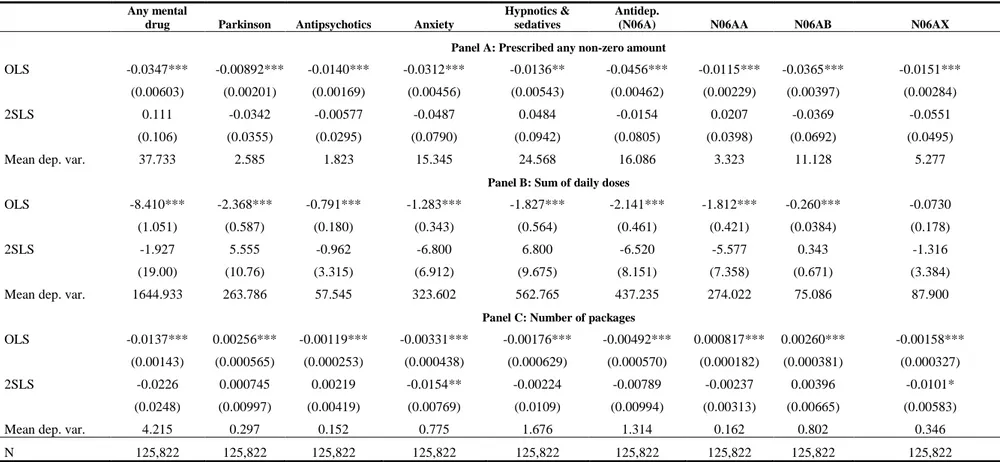
Results from the IV analysis are reported separately for drug prescriptions, hospital admissions and mortality. I document no effect on the probability of being prescribed a non-zero quantity of drugs, nor on total drug consumption. There is also no effect on the probability of being hospitalized due to any cause, nor on the number of days spent in hospital. Moreover, tracking mortality up to year 2011 (age 76 for the oldest cohort), I fail to reject the null hypothesis of no causal effect of working longer on mortality. The coefficients are relatively precisely estimated, which allows me to bound the effect sizes to a narrow range around zero. The main results are supported by several robustness tests.
There are some exceptions to the overall pattern of null results. First, I find suggestive evidence that postponing retirement causes a reduction in the number of prescribed packages of drugs that treat anxiety. Because there is no corresponding effect for the extensive margin, this suggests that postponing retirement might alleviate short-term anxiety and depressive symptoms among elderly with pre-existing mental health issues. I also find that postponing retirement reduces the likelihood of being treated for diabetes and diseases of the circulatory system. These results are, however, not robust to model specification and outcome measurement and should therefore be interpreted with caution.
The identification strategy rests on the assumption that there is no link between retirement age and health arising from the interaction of time and treatment status, as this would violate the parallel trends assumption. I explore the validity of this assumption by comparing pre-reform trends in mortality and health care utilization between the treatment and control group. Most health outcomes develop similarly prior to the reform, but there are a few exceptions. Hence, we cannot rule out the existence of different time-trends that mask a causal relationship between retirement and health, but the evidence that justifies the parallel trends assumption is relatively strong.
Although the empirical framework is based on Swedish public sector workers, the results should be of more general interest. First, the worker categories that were affected by the reform are characterized by demanding work environment and relatively high rates of sickness absence, including personal care workers, nursing professionals, cleaners and restaurant service workers. The focus on low- to medium-paid public sector jobs is relevant from a policy perspective since various discussions of increasing
the retirement age thresholds deal primarily with the concern that such increases could adversely affect individuals in low-skilled jobs. Second, since retirees have equal access to publicly provided health service and medical care as employed individuals, the estimates are likely to capture the direct effect of working longer on health care utilization and mortality, rather than indirect effects, such as access to health insurance. The effects are also unlikely to operate through a loss of income as the long-run effect of the reform on disposable income is small. Finally, health care utilization is arguably the most important health dimension in estimating the fiscal impact of reforms that promote longer working lives. In 2014, individuals aged 65 and over comprised 20 percent of the Swedish population, but they accounted for 40 percent of total drug prescriptions and 47 percent of all patient discharges from public hospitals (Socialstyrelsen, 2015a, 2015b). There is a risk that the utilization of health care might reflect other factors than the need for health care, such as ability to pay and patient proximity to the medical center. However, the study of outcomes severe enough to require hospital inpatient care or that lead to death should diminish this risk.
The remaining part of the paper is organized as follows. Section 2 discusses the previous literature; Section 3 discusses the details of the reform; Section 4 describes the data; Section 5 outlines the econometric framework; Sections 6 and 7 present first and second-stage results, respectively; Section 8 presents additional results; and Section 9 concludes.
2 Previous literature
This paper relates more broadly to a literature that tries to estimate the causal effect of retirement on health. To get a picture of the results in this literature, Table A2 gives a brief summary of the empirical methods and key findings of 25 selected articles in the health-economic literature. Two of these studies report zero effects of retirement. Thirteen studies report that retirement has a positive effect on health, whereas the remaining ten conclude that retirement is in fact associated with a decline in health. Even though these papers differ along several important dimensions, such as the population being studied, health outcomes and empirical methodology, these contrasting results are also likely to stem from the lack of convincing empirical strategies to deal with endogenous selection into retirement.
The most frequently used instrument is age-specific retirement incentives, such as early retirement windows or eligibility age-thresholds. This strategy has been used both in cross-country studies (e.g Coe and Zamarro (2011); Heller-Sahlgren (2016); Mazzonna and Peracchi (2012); Rohwedder and Willis (2010); Sahlgren (2012)) and in within-country studies (e.g. Behncke (2012); Bonsang et al. (2012); Bound and Waidmann (2007); Gorry et al. (2015); Neuman (2008)). The identifying assumption is that the instruments affect health only indirectly through their effects on the age of retirement. This is a strong assumption for several reasons. First, workers who anticipate that there are financial incentives to retire at a certain age may adjust their behavior before retirement (Coe and Lindeboom, 2008). Second, absent any behavioral response, workers who are subject to different retirement rules may differ with respect to unobserved variables (Kuhn et al., 2010). For example, individuals with a bad latent health state might be more likely to choose jobs where they can retire early. Third, reaching the eligibility age or the normal retirement age may have a direct impact on health if it is considered a milestone in a person's life (Behncke, 2012).
Researchers have turned to reform-based variation in retirement timing to deal with these issues. Comparing individuals affected by a reform to individuals who are not means that we do not have to worry about the underlying reasons why individuals chose their respective occupation in the first place. This approach also overcomes the issue of individuals adjusting their behavior before retiring, provided that the reform is not fully anticipated by the individuals. The reform studied in this paper was announced only one year prior to its implementation, therefore giving workers little opportunity to increase their retirement income in ways other than retiring later.
A crucial assumption for the reform-based approach is that the reform is exogenous with respect to individuals' health status, i.e. that the reform affects health only through retirement. This assumption might be violated if the reform impacts health before individuals retire. For example, Grip et al. (2012) show that the mental health of Dutch public sector workers deteriorated as a result of a substantial reduction in their pension rights. In the context of this paper, raising the normal retirement age with short notice might have been perceived as unfair, which may have impacted (mental) health negatively. However, this possibility is unlikely to pose a problem for this study because of the strong norm of retiring at the age of 65 that prevailed in Sweden at the
time. The new retirement age for the affected workers was already the normal retirement age in all other occupational pension plans, both in the public and private sector. This should have played down feelings of disappointment and frustration among the affected local government workers.
3 The occupational pension system
3.1 Retirement benefits in Sweden
Sweden's pension system has two main pillars, a universal public pension system and an occupational pension system. Swedish retirees generally receive most of their pension income from the public pension system, but the occupational pension system is an important complement. The occupational pension system consists of a number of different pension plans that are negotiated at the union-level and cover large groups of workers. In fact, the four largest agreement-based occupational pension plans cover around 90 percent of the total work force. These include the pension plan for blue-collar private sector workers, white-collar private sector workers, local government workers and state-level government workers, respectively. The focus of this study is the pension plan for local government workers. The control group is made up of private sector workers. For the cohorts being studied, i.e. 1935 to 1942, there were no major changes in the private sector pension plans and they all faced a normal retirement age of 65.4
3.2 The occupational pension reform for local government workers
The pre-reform occupational pension plan for local government workers, called PA-KL, covered local government workers born before January 1, 1938. PA-KL was defined benefit and directly coordinated with the public pension system. PA-KL stipulated that the sum of the annual occupational pension benefit and the public pension benefit should amount to a certain fraction of the individual's pre-retirement income. The occupational pension would always pay out the residual amount net of the public pension benefit to reach a certain replacement rate. In year 2000, the gross replacement rate amounted to 73 percent for a female local government employee with an average
4 There are two large occupational pension plans in the private sector: one for blue-collar workers (SAF-LO) and one for white-collar workers (ITP). The ITP plan was mainly defined benefit and the same rules applied to all birth cohorts studied in this paper. The SAF-LO plan, on the other hand, is a pure defined contribution scheme. The implementation of the SAF-LO plan in 1996 implied that blue-collar workers born between 1932 and 1967 were subject to special transitional rules. However, cross-cohort differences in retirement incentives are minor because of the long transition period. See Hagen (2013) for a more detailed description of these pension plans.
wage rate who retired at the age of 63. If the public pension accounted for 60 percent, the occupational pension benefit would amount to 13 percent of her qualifying income. Thus, local government workers only needed to know about the gross replacement rates to get a full picture of their retirement income.5
In the pre-reform pension plan, retirement was mandatory for everyone at the age of 65 unless the employer offered a prolongation. However, the age at which full or unreduced retirement benefits could be withdrawn, i.e. the normal retirement age (NRA), was different for different occupations. The NRA was either 63 or 65. Early withdrawals could be made from the age of 60, but the penalty rate at a given claiming age, i.e. the reduction in the gross replacement rate, was different depending on what NRA the worker faced. Here, I focus on workers who had a NRA of 63.
Workers who faced a NRA of 63 could retire at this age with a full benefit. The benefit was not actuarially increased for claims made after 63, which means they had little incentive to work past this age. Selin (2012) shows that these workers lost SEK 169,000 (USD 1 = SEK 7.2 in 2010) in pension wealth from continuing working an additional year after turning 63. Broad categories of workers had a NRA of 63, including personal care workers, nurses, pre-school teachers, restaurant service workers and cleaners.
In 1998 a new agreement, PFA98, was signed for Swedish local government workers. The most important change was that the NRA was set to 65 for all local government workers. This was achieved by introducing equal early retirement penalty rates for all occupations. The new penalty rates implied that the pension was reduced by 0.4 percent per month of retirement before age 65. Rather than receiving a full benefit, retiring at age 63 as compared to 65 now implied a substantial benefit reduction of 9.6 percent (0.4×12×2=9.6).
The reform implied two additional changes to the pension plan. First, there was a partial shift from defined benefit to defined contribution. For earnings below the ceiling of 7.5 increased price base amounts, the pension was entirely defined contribution.6 The contribution differed slightly over time and also between employers and type of tenure, but centered on 3.4 – 3.5 percent for wage portions below the income ceiling and 1 – 1.1 percent for earnings above. Individuals with earnings above the ceiling got an
5
Selin (2012) has used this reform to study spousal spillover effects on retirement behavior. 6
additional defined benefit pension.7 The individual could always increase her pension wealth by postponing retirement until the age when she was obliged to retire or until no more pension rights could be earned. Second, the occupational pension was not residual to the public pension anymore, but paid out as a separate entity. Workers in the new plan were thus directly exposed to the early retirement penalty rates in the public pension system.8
The new PFA98 agreement came into effect on January 1, 2000 for those born in 1938 or later. Those born in 1937 and earlier were completely unaffected by the occupational reform and would still be covered by the old plan. The reform was implemented rather quickly and without much media coverage.9 The purpose of the reform was to harmonize rules across all worker categories in the local government sector and to adjust rules to the new defined contribution structure.
While the reform substantially increased the incentives to postpone retirement beyond the age of 63, it did not change the stock of already accumulated occupational pension wealth. The reason for this was a transition rule that would compensate workers in post-reform cohorts for potential benefit reductions due to the new rules. The pension wealth earned up to December 31, 1997 was converted into a life annuity that corresponded to the annual pension benefit that the individual would have received if she had retired by that date. Pension rights earned after this date were accredited the new pension plan. If the resulting pension from these two components was lower than the corresponding pension in the absence of a reform, workers received the difference from the employer. As a result, the pension wealth at age 65 was more or less unchanged for the transition cohorts. Importantly, workers who retired before 65 were not eligible for this compensation, which implies that the most important effect of the reform was to raise the NRA from 63 to 65 for workers who had a NRA of 63 in the pre-reform pension plan.
It should be noted that the first post-reform cohort in the empirical analysis, i.e. those born in 1938, are also the first cohort to participate in the new public pension system.
7
This defined benefit component amounted to 62.5 percent of earnings between 7.5 and 20 base amounts and 31.25 percent between 20 and 30 base amounts.
8
The monthly penalty rate in the public pension system was 0.5 percent.
9 Selin (2012) reports that a search in the online press archive Presstext, which covers the biggest daily newspapers in Sweden, reveals that the first article mentioning PFA98 is written in the fall of year 2000. Low media coverage, however, does not rule out the possibility that the reform may have become known among the affected individuals through unions informing or word-of-mouth information.
The 1938 cohort receives one-fifth of its benefit from the new system and four-fifths from the old system. Each cohort then increases its participation in the new system by 1/20, so that those born in 1954 will participate only in the new system (Hagen, 2013). Benefits from the new system were paid out for the first time in 2001, three years after it was legislated. The transition rules apply to all individuals born after 1937 and are controlled for in the empirical analysis by including cohort fixed-effects in the regression model.
4 Data
4.1 Data on retirements
Individual demographics and labor market information is collected and maintained by Statistics Sweden. The Longitudinal Database on Education, Income and Employment (LOUISE) provides demographic and socioeconomic information. The data covers the entire Swedish population between 16 and 65 during the period 1987–2000, and individuals aged 16 to 74 between 2001 and 2010. The population of interest is local government workers whose NRA was increased from 63 to 65 in 2000. The main sample analyzed is composed of individuals born between 1935 and 1942. Those born in 1938 were the first ones to be affected by the new rules. The control group is made up of private sector workers in the same birth cohorts. The private sector workers faced a normal retirement age of 65 both before and after the local government pension reform.
Importantly, there is information in the data which allows me to distinguish these workers from other workers in the local government sector who had a NRA of 65 both before and after the reform. I use the Swedish Standard Classification of Occupations (SSYK-96) to identify workers in occupations who had a NRA of 63.10 Individuals who are observed working in any of these occupations between ages 61 and 63 are included in the treatment group. I identify workers with a NRA of 65 in the same way. If an individual is observed working in both occupation categories, I use the most recent observation to determine the NRA. SSYK codes are available from 1996, which means that those born in 1935 are the oldest cohort for whom occupation status is known at
10
Standard för svensk yrkesklassificering (SSYK-96). SSYK-96 is based on the International Standard Classification of Occupations (ISCO-88).
age 61.11 I define someone as working in the private sector if she has not been employed in the public sector between ages 61–63. It is more difficult to determine private sector affiliation from the data. The data which contain the SSYK codes only contain a small representative sample of private sectors workers (around 23 percent). In contrast, the universe of public sector workers is included in this data.
I make four restrictions to the sample of local government and private sector workers born between 1935 and 1942. First, because the affected worker categories in the local government sector were dominated by women, male workers are excluded from the analysis. In fact, only 3 percent of these workers are men. Second, I restrict the analysis to individuals registered as employed for 12 full months in the year of their 61st birthday. This restriction is done for two reasons. First, it excludes individuals who exited the labor force early and whose retirement decision is unlikely to have been affected much by the reform. Second, it ensures that I observe at least one SSYK code for each local government worker. In order for the SSYK code to be reported, the individual must be employed during the "reference month", which typically occurs at the end of the year. In effect, this restriction implies that the first month in which individuals are allowed to retire is the month in which they turn 62. Third, I restrict the sample to individuals who have five years of consecutive employment prior to age 61 (at any work place).12 Finally, I also exclude individuals who are registered as self-employed at some point between ages 61 and 63. The final sample consists of 133,026 individuals of whom 57,415 are local government workers.
Table 1 reports the distribution of workers in the most numerous worker categories, and the corresponding SSYK codes, in the treatment and control group, respectively. The majority of the treatment group work within personal care. These include child-care workers, assistant nurses, home-based personal care assistants and dental nurses. Other important worker categories in the treatment group are restaurant service workers, nursing professionals and cleaners. The number of worker categories in the control group is larger since it includes both blue-collar and white-collar workers in the private sector. The most numerous worker categories in the control group are blue-collar jobs,
11
It is not possible to determine the NRA for all local government workers. The NRA cannot be determined for SSYK codes that map simultaneously to occupations with different NRAs. For example, pre-school teachers and after-school teachers have the same SSYK code (3310), but different NRAs. I therefore restrict the treatment group to workers in occupations where the SSYK code maps exclusively to a NRA of 63.
12
including salespersons, plant and machine operators, manufacturing laborers and craft workers. White-collar workers are foremost represented in the categories "other associate professionals", "professionals" while "clerks" include both. Three of the treatment group occupations are found in the control group, too (personal care-related workers, restaurant service workers, and helpers and cleaners).
Table 1. Occupations in the treatment and control group
Treatment group (local government) Control group (private sector)
Occupation SSYK-96 Occupation SSYK-96
Personal care & related workers (64%) 513 Salespersons (31%) 52 Restaurant service, housekeeping (15%) 512, 913 Plant & machine operators (15%) 8 Nursing & midwifery professionals (13%) 223, 323 Clerks (16%) 4 Helpers & cleaners (8%) 912 Manufacturing laborers (6%) 932 Physiotherapists (<1%) 5141 Helpers & cleaners (9%) 912 Hairdressers (<1%) 3226 Craft & related trade workers (6%) 7
Restaurant service, housekeeping (7%) 512, 913 Other associate professionals (3%) 34 Personal care & related workers (3%) 513 Professionals (2%) 2
Note: The first column reports the occupations in the local government sector that had a NRA of 63 before the reform (the treatment group). The third column reports the most common private sector occupations (the control group). The corresponding SSYK codes are listed in the second and fourth columns, respectively. The share of workers in each occupation is reported in parentheses. A worker is classified into an occupation if she is observed working in that occupation at any time between ages 61–63. The occupations are therefore not mutually exclusive. SSYK codes are only available for a representative sample of the private sector workers. The shares in this group are adjusted for sampling probabilities.
The retirement definition reflects the month in which an individual retires completely from the work force. This definition uses records of employment spells, which are obtained from the Register-Based Labor Market Statistics (RAMS). The information in RAMS is based on reports that all employers submit to the Swedish Tax Agency. For each employee, the employer must report how much wages and benefits have been paid out, how much taxes have been drawn and, most importantly, during which months the employee has been employed at the firm. This information allows me to infer in what month and year an individual exits the labor market. The decision to retire is equated with the month in which the individual's last employer reports the employment contract to be officially ended. The outcome variable in the first-stage analysis on the retirement effects of the reform is defined as the number of months an individual is registered as
employed between ages 62 and 68. The upper limit of age 68 is chosen because it is the oldest age to which the youngest cohort can be tracked.13
4.2 Data on health care utilization and mortality
I study mortality outcomes and two major types of health care utilization: hospital-lizations and consumption of prescription drugs. Three register based data sources are used for this purpose.
The analyses of drug prescriptions are based on data from the Prescription Drug
Register, which contains information about all over-the-counter sales of prescribed
medical drugs between 2005 and 2009. For each occasion when a prescription drug was bought, the data contains detailed information about the Anatomical Therapeutic Chemical (ATC) code of the drug, and the number of defined daily doses (DDDs) purchased over the entire period. The analysis of mortality is based on information from the Cause of Death Register. Causes of death are classified using the International Classification of Diseases (ICD). Hospitalizations are studied using information about inpatient care available in the National Patient Register.14 For each hospitalization event, the register has information about the arrival and discharge date, and diagnoses codes in ICD format. Inpatient records exist from 1964 to 2010, while the mortality data ends in 2011.
The analysis focuses on the extensive and the intensive margins of health care utilization. For the extensive margin, I define a set of binary outcome variables that equal 1 if the individual consumes a non-zero quantity of drugs or is hospitalized for at least one night during a pre-specified time period. The intensive margin outcome variables for drug prescriptions are given by the product of the DDD per package and the number of prescribed packages, summed over the years 2005–2009 for each individual. Since DDDs are not directly comparable across drug types, I complement this analysis by looking only at the prescribed number of packages. Information on the number of days spent in hospital is used to construct intensive margin outcomes for
13
The employer records have been used in the Swedish context by Laun (2012). She studies the retirement effects of two age-targeted tax credits in 2007 using the number of remunerated months at age 65. Kreiner et al. (2014) use monthly payroll data on wages and salaries to study year-end tax planning in Denmark. A similar definition of retirement is also used in the Austrian context by Kuhn et al. (2010) and Manoli and Weber (2014).
14 Information on hospital admissions is provided by the National Board of Health and Welfare and covers all inpatient medical contacts at public hospitals from 1987 through 1996. From 1997 onward, the register also includes privately operated health care. Before 1997, virtually all medical care in Sweden was performed by public agents (Hallberg et al., 2015)
inpatient care. The intensive margin adds important variation to the quantity of consumed health care, especially for individuals with previous records of health care utilization.
Because the different health registers cover different years, the pre-specified time period over which health outcomes are defined will vary across the type of health event. The mortality data ends in 2011, which means that the maximum age up to which all cohorts can be tracked is 69. The outcome variable is thus set equal to 1 if the individual died before reaching this age. To make use of all the data at hand, I also look at mortality by year 2011. In a similar fashion, the hospitalization outcomes are either based on an individual's hospital admissions between ages 65 and 68 or between age 65 and year 2010. The latter time period implies that the length of the follow-up period decreases with the year of birth of the individual. Age 65 is chosen as the lower age limit because our primary interest lies in estimating the effects on health care utilization after the individual is retired. Finally, all drug outcomes are based on prescriptions made between 2005 and 2009.
I adopt a framework used by Cesarini et al. (2015) to classify mortality and health care utilization events into a number of relevant medical causes. Specifically, I examine deaths and health care utilization events into two cause categories: common causes and hypotheses-based causes. The common causes are cancer, respiratory disease, diseases of the circulatory system and other. The hypotheses-based causes are chosen based on their appearance in previous economic and medical literature on the association between retirement and health. These include ischemic heart disease, hypertension, cerebrovascular disease15, musculoskeletal disease, alcohol and tobacco consumption, injury and type 2 diabetes. While the common causes are the same, Cesarini et al. (2015) choose the hypotheses-based causes based on their known relationship with wealth rather than retirement.
Mortalities and hospital admissions are readily classified into each of these causes using the ICD codes. Only primary diagnoses are used to classify hospital admissions and deaths into one of the common causes. These are therefore mutually exclusive. In the hypotheses-based causes, the cause-of-death or hospitalization variable is set equal to 1 if the condition matches at least one of the (first five) listed diagnosis codes on the
15
Cerebrovascular disease refers to a group of conditions that affect the circulation of blood to the brain, causing limited or no blood flow to affected areas of the brain. This is commonly a stroke.
discharge record or the death certificate. All codes are included because some of the hypotheses-based causes are rarely listed as the primary cause of death or primary diagnosis.
I use the ATC codes to classify prescription drugs into categories that closely resemble the common causes and hypotheses-based causes.16 The prescription data is also used to define a number of (hypotheses-based) mental illnesses. These include depression, psychosis, anxiety, sleeping disorders and Parkinson. Table A1 describes the aggregation of ATC and ICD codes for each cause.
A concern with using health care data is that the utilization of health care might reflect other factors than the need for health care (Doorslaer et al., 2004; Van Doorslaer et al., 2000). One such factor is ability to pay. In principle, receiving care must not be influenced by the ability to pay since most medical service expenses in Sweden are covered by taxes. There is, however, evidence that there exists pro-rich inequity in the utilization of health care. I diminish this risk by studying both the consumption of prescription drugs, where such inequity is likely to play a role, and outcomes severe enough to require hospital inpatient care. Another potential factor is differences in time availability between retirees and workers. Those who work longer as a result of the reform face a higher non-monetary cost of seeking health care. To make sure that the treatment and control group face similar time constraints, I focus on health care received after the age of 65 when most individuals are retired.17. Again, focusing on severe outcomes that either require inpatient care or lead to death should also play down the importance of help-seeking behavior associated with time availability.
4.3 Descriptive statistics
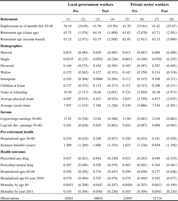
Table 2 shows descriptive statistics for pre- and post-reform cohorts for the treatment and control group, respectively.
The first row shows that post-reform cohorts in the treatment group retire about 5.5 months later than the pre-reform cohorts. The corresponding difference in the control group is very small, which yields a raw difference-in-differences (DD) estimate of 5.3
16
The hypotheses-based classification is amended in several ways. First, following Cesarini et al. (2015), I merge ischemic heart disease and hypertension into a single category ("Heart") because many drugs are used to treat both these illnesses. Second, I limit the set of drugs used to treat musculoskeletal diseases (ATC code "M") to analgesics (painkillers). Third, I do not try to classify drugs into "Alcohol and Tobacco" due to the complexity of the prescription data.
17
The only case where I track health outcomes before the age of 65 is drug utilization for those born in 1941 and 1942 (the prescription data starts in 2005).
months. This is strong preliminary evidence that the reform had a positive impact on the retirement age. The second and third rows show that similar results are obtained for two alternative measures of retirement. According to the first alternative definition, individuals who receive a positive amount of pension income are classified as retired. The second definition is income-based. According to this definition, the individual retires the year before her annual earnings fall below 1 price base amount (≈USD 5,900 in 2010). Since these definitions are measured at the yearly level, the raw DD estimate in the second row of 0.56 reflects an increase in the claiming age of more than 6.5 months. The income-based definition of retirement reflects a smaller, yet sizable, effect of about 3 months.18
Table 2 shows that the two groups are similar in terms of several background characteristics, including marital status, the probability of having children (of any age) at home and immigrant status. The two groups also have similar pre-retirement health status. Sickness absence, measured as the number of years an individual has been absent from work for more than 14 consecutive days between ages 56 and 60, is only marginally higher in the treatment group, just like the probability of having been hospitalized during the same period.19 Differences apply mainly to education level and pre-retirement earnings. Local government workers have, on average, 0.5–0.6 years more of schooling and somewhat higher pre-retirement earnings than the private sector workers. The income distribution of the local government workers is, however, more compressed.
18
Individuals are allowed to be retired from the age of 56 according to these definitions, which helps explain why the average retirement ages implied by these definitions are lower than the average retirement age implied by the main definition. The sample restrictions explained in section 4 apply nonetheless.
19 Specifically, our measure of sickness absence is the number of years the variable "sjukpp" in the LOUISE database takes on a non-zero positive value between ages 56 and 60. "Sjukpp" includes sickness benefits that are paid out by the Swedish Social Insurance Agency (Försäkringskassan). The Social Insurance Agency is responsible for paying out sickness benefits to individuals who have been sick for more than 14 consecutive days.
Table 2. Descriptive statistics
Local government workers Private sector workers
Pre Post Pre Post
Retirement (1) (2) (3) (4) (5) (6) (7) (8) Employment nr of months btw 62-68 36.19 (24.09) 41.56 (21.85) 41.30 (23.61) 41.42 (23.07)
Retirement age (claim age) 63.75 (1.976) 64.19 (1.808) 63.83 (2.478) 63.71 (2.501)
Retirement age (income-based) 63.23 (2.071) 63.75 (2.508) 62.95 (2.911) 63.23 (3.089)
Demographics Married 0.623 (0.485) 0.620 (0.485) 0.613 (0.487) 0.609 (0.488) Single 0.0535 (0.225) 0.0592 (0.236) 0.0612 (0.240) 0.0702 (0.255) Divorced 0.169 (0.375) 0.194 (0.395) 0.183 (0.387) 0.207 (0.405) Widow 0.155 (0.362) 0.127 (0.333) 0.143 (0.350) 0.114 (0.318) Immigrant 0.103 (0.304) 0.0886 (0.284) 0.112 (0.315) 0.108 (0.311) Children at home 0.127 (0.333) 0.113 (0.317) 0.112 (0.315) 0.108 (0.311) Years of schooling 10.30 (2.717) 10.69 (2.691) 9.724 (2.859) 10.38 (2.973)
Average physical strain 6.497 (0.915) 6.421 (0.925) 5.623 (2.559) 6.873 (2.035)
Average social strain 7.597 (1.233) 7.348 (1.326) 6.149 (3.086) 7.536 (2.501)
Income
Log(average earnings 56-60) 11.92 (0.336) 12.04 (0.368) 11.88 (0.681) 12.04 (0.682)
Log(std. dev. earnings 56-60) 9.261 (0.838) 9.645 (0.802) 9.624 (0.987) 9.888 (0.965)
Pre-retirement health
Hospitalized ages 56-60 0.254 (0.435) 0.240 (0.427) 0.250 (0.433) 0.241 (0.428)
Sickness benefits (years) 1.209 (1.269) 1.000 (1.235) 1.023 (1.236) 0.838 (1.196)
Health outcomes
Prescribed any drug 0.927 (0.261) 0.944 (0.230) 0.925 (0.263) 0.949 (0.219)
Prescribed mental drug 0.397 (0.489) 0.358 (0.479) 0.403 (0.491) 0.364 (0.481)
Hospitalized ages 65-68 0.294 (0.456) 0.276 (0.447) 0.299 (0.458) 0.277 (0.448)
Hospitalized age 65-year 2010 0.578 (0.494) 0.355 (0.478) 0.579 (0.494) 0.352 (0.477)
Mortality by age 69 0.0453 (0.208) 0.0447 (0.207) 0.0450 (0.207) 0.0413 (0.199)
Mortality by year 2011 0.103 (0.304) 0.0561 (0.230) 0.103 (0.304) 0.0541 (0.226)
Observations 18561 38854 23895 51716
Note: The sample includes female local government (treatment group) and private sector (control group) workers born between 1935–1942 who have five years of consecutive employment prior to age 61 (at any work place) and are registered as employed for 12 full months in the year of their 61st birthday. The sample of local government workers is restricted to workers in occupations whose NRA was increased from 63 to 65 in 2000. Earnings are in the 2010 price level. Retirement variables right-censored at age 68. Columns (1)–(4) display statistics for the treatment group, while columns (5)–(8) consider the control group. Standard deviations in parentheses. Pre-reform cohorts refer to those born before 1938.
Table 2 gives some idea about how these characteristics change over time in the treatment and control group, respectively. To estimate these changes more formally, I employ a DD framework and regress the characteristic of interest on several interaction terms between cohort (j=1935,...,1942) and the local government dummy as well as the
local government dummy itself and cohort-fixed effects (the 1937 cohort as reference). The estimated interaction terms are reported in Table A3. The results give little reason to be concerned about differential trends with respect to most background characteristics and pre-retirement inpatient care. However, two things should be pointed out. First, it is clear that the level of education in the treatment group increases at a slower rate than in the control group. The differential trend with respect to education generates important differences also in terms of pre-retirement earnings, at least for the three youngest cohorts. I will account for these trends in the regression analysis by including interaction terms between education/income and birth cohort and sector. Second, the pre-reform cohorts in the treatment group exhibit higher levels of sickness absence prior to retirement. Post-reform differences in sickness absence are, however, much smaller and in most cases insignificant.
Turning to our health outcomes, we see that around 30 percent of the local government workers are hospitalized for at least one night between ages 65 and 68. This fraction increases to almost 60 percent when the follow-up period is extended to year 2010. The private sector workers exhibit very similar hospitalization rates. The differences amount to less than one percentage point. The two groups are also similar with respect to drug consumption. More than 90 percent of the individuals in the pre-reform cohorts are prescribed a non-zero quantity of drugs between 2005 and 2009. Around 40 percent are prescribed mental drugs. Note, however, that the cross-cohort decline in drug consumption and hospital admissions is larger in the treatment group than in the control group. The opposite pattern is seen for our two measures of mortality, i.e. the probability of being dead by the age of 69 or by year 2011. In sum, it is difficult to draw any conclusions about the existence of an effect of the reform on mortality and health care utilization based on these raw DD estimates.
5 Econometric framework
The primary interest of this paper is to estimate the health effects of postponing retirement. The regression model of interest can be written as:
yi=α+βRi+ϵi (1)
where y
i is a measure of health for individual i and ϵiis the error term. 𝑅𝑖 is a continuous
employment between ages 62 and 68 conditional on being employed at the age of 61. The coefficient of interest is β, the causal effect of an additional month of employment on health. Ri is endogenous because individuals who retire later are more likely to be in good health.
To estimate the causal effect of continued work we need variation in retirement timing that is exogenous to health. For this purpose I utilize the above described reform, which raised the NRA from 63 to 65 for local government workers born in 1938 or later. I use an instrumental variable (IV) framework to assess the causal relationship between postponing retirement and health, where 𝑅𝑖 is instrumented by an interaction term between being born in 1938 or later (post-reform cohorts, (CH=1) and being employed in the local government sector (LG=1).This means that I estimate the causal effect for those individuals who postpone retirement due to the reform, i.e. the compliers. Assuming heterogeneous effects of postponing retirement on health, the 2SLS estimator estimates the local average treatment effect (LATE) instead of the average treatment effect (ATE).
For individual 𝑖 in cohort 𝑗 in sector 𝑠, the first-stage DD equation is then written as
Ri,j,s=α+δ�LGs×CHj∈[1938,1942]�+ϕLGs+λj+Xi,j,sθ+ui,j,s (2)
where 𝜆 denotes cohort-fixed effects and the vector Xi,j,s is a set of control variables which includes the number of years of schooling, region of residence and month of birth fixed-effects, dummies for being single, divorced or widowed (married reference group), immigrant status and having children at home. The set of control variables also include the log of the average of yearly earnings, the log of the standard deviation of yearly earnings and the number of years with more than 14 consecutive sick leave days between ages 56 and 60. To account for differential trends in educational attainment/income, I also add interactions between years of schooling/income and cohort and years of schooling/income and local government. The coefficient of interest is 𝛿, which reflects the reform effect on the number of months employed before exiting the labor market, comparing local government workers born in 1938 or later to private sector workers in the same birth cohorts. Differences in employment across the treatment and control group are captured by the term ϕ. The maximum value of Ri,j,s is 72 because of right-censoring at age 68.
To capture the heterogeneity in the effect of the instrument on the first-stage outcome, I allow for cohort-specific effects by including interaction terms between the local government dummy and cohort 𝑗 in the first-stage equation
Ri,j,s=α+ � δj
j
�LGs×CHj∈[1938,1942]�+ϕLGs+λj+Xi,j,sθ+ei,j,s (3)
which implies there are five instruments for the main specification (post-reform cohorts: 1938-1942). Each cohort-specific reform effect δ is evaluated against a pooled sample of the pre-reform cohorts.20 The IV model is just-identified if the first-stage equation is given by (2). The model is over-identified if the first-stage equation is given by (3), i.e. the number of instruments is larger than number of endogenous regressors. The over-identified model better captures the causal effect of postponing retirement if there are differences across birth cohorts in their retirement response to the reform. The causal effect from the over-identified model averages IV estimates using the instruments one at a time, where the weights depend on the relative strength of each instrument in the first stage.
The reduced-form is given by replacing the dependent variable in any of the first-stage equations by a measure of health, yi,j,s The reduced-form equation for the
just-identified model is then given by
yi,j,s=α+ψ�LGs×CHj∈[1938,1942]�+ϕLGs+λj+Xi,j,sθ+ui,j,s (4)
The reduced-form estimate ψ is referred to as the intention-to-treat effect. This specification is similar to a DD model, where we compare health outcomes of local government workers and private sector workers across birth cohorts.
5.1 Identifying assumptions
Technically, identification requires two assumptions. First, the increase in the NRA must have an impact on the retirement age, that is δ≠0 in Equation (2) (instrument relevance). This assumption is carefully analyzed in section 6. The impact of the reform on retirement. Second, exposure to the increase in the NRA affects health only through the number of months in employment (the exclusion restriction). This means that the instrument must be uncorrelated with the error term in the second-stage equation.
20
This specification is analogous to the specification by Atalay and Barrett (2014b) who study the impact of age pension eligibility age on retirement in Australia with the difference that they exploit variation in birth cohort and gender rather than birth cohort and sector as this paper does.
Concerns about the existence of other channels through which the reform might affect health can be alleviated if we can show that the parallel trends assumption hold. This assumption implies that the outcome variable evolved in the same way in the treated group as in the control group in absence of the reform. Figure 1 plots series of average outcomes for the treatment and control group before and after the reform for some of the key health measures.
Figure 1. Comparing the treatment and control group
Note: This figure plots the means and the corresponding 95 percent confidence intervals of several health outcomes by cohort and treatment status. Solid and dashed lines refer to the treatment and control group, respectively. The confidence interval is obtained by regressing each health outcome on a constant, separately by cohort and treatment status.
The two top panels show that the probability of being prescribed a non-zero quantity of drugs evolved similarly for pre-reform cohorts in the two groups. The lower panels show that post-retirement hospitalization and mortality also seem to satisfy the parallel trends assumption. It is also reassuring that the levels are similar across the two groups.
We can test the parallel trends assumption more formally by estimating pre-reform trends in the reduced-form framework. Specifically, I extend Equation (4) by adding two interaction terms between the local government dummy and cohorts (j=1936, 1937). For the parallel trends assumption to hold, the estimated δj coefficients
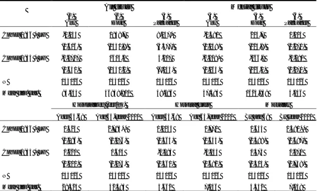
for these two cohorts should be close to zero and insignificant. Table 3 reports the estimation results for the extensive margin health outcomes shown in Figure 1 along with the corresponding intensive margin measures of health care utilization.
Table 3. Estimating pre-reform trends in health care utilization and mortality
All drugs Mental drugs
(1) Any (2) Dose (3) Packages (4) Any (5) Dose (6) Packages Cohort 1936 * LG -0.135 1858.7 8.157* -0.481 204.7 0.104 (0.606) (1531.9) (4.377) (1.149) (225.9) (0.270) Cohort 1935 * LG -0.0717 1615.0 5.207 -2.109* -166.9 -0.290 (0.631) (1551.2) (7.045) (1.165) (226.1) (0.270) N 133026 133026 133026 133026 133026 133026
Mean dep. var. 94.033 46848.811 48.086 37.384 1623.839 4.146
Hospitalized (yes/no) Hospital days Mortality Ages 65-68 Age 65-year 2010 Ages 65-68 Age 65-year 2010 By age 69 By year 2011
Cohort 1936 * LG 1.423 2.783** 0.0135 0.771 0.643 1.591**
(1.086) (1.176) (0.365) (0.645) (0.488) (0.697)
Cohort 1935 * LG 1.220 1.615 -0.194 -0.155 0.473 0.170
(1.101) (1.175) (0.360) (0.682) (0.505) (0.738)
N 133026 133026 133026 133026 133026 133026
Mean dep. var. 28.325 42.484 3.662 7.146 4.352 7.038
Note: This table shows estimates from estimating Equation (3) after adding two pre-reform interaction terms between cohort 𝑗 = (1935, 1936) and the local government dummy. See Table 2 and Table 4 for more information on the sample of analysis and controls. Robust standard errors in parentheses. ***, **, * denote statistical significance at the 1%, 5% and 10% level respectively.
The upper panel of Table 3 shows that the pre-reform trends with respect to drug consumption are similar. Only two of the coefficients are statistically different from zero (at the 10 percent level) and they also relate to different cohorts. The lower panel raises some concern of a positive trend in the health status of the treatment group individuals as two of the estimates for the 1936 cohort are positive and significant; the probability of having been hospitalized between age 65 and year 2010 and mortality by year 2011. This pattern is similar to what we found in section 4.3 for sickness absence prior to retirement and calls for caution when interpreting the results. However, all other hospitalization variables are insignificant and there are also large year-to-year fluctuations in mortality. Moreover, none of the pre-reform interaction terms in Table 3 are jointly significant at the 5 percent level.
The exclusion restriction could nonetheless be violated if the reform coincides with differential trends in occupation-specific work environment. One concern for the
existence of differential trends in work environment between public sector and private sector occupations is the large scale retrenchment of the public sector that followed the financial crisis that unfolded in the early 1990s (Angelov et al., 2011) . While the effect on private sector employment was large and immediate, the effect on public sector employment was more protracted (Lundborg, 2001). If the work environment deteriorated across cohorts in the treatment group as a result of this, and there was no corresponding decline in the control group, we might capture effects on post-retirement health that are not only due to continued work, but to changes in work environment, too. I do two things to investigate this issue. First, I look at occupation-specific sick leave patterns for women around the reform. Using data from the Social Insurance Agency, the upper panel of Figure 1 plots the fraction of female workers that were absent from work for more than 60 days in a given year for five important worker categories. Personal care workers, the most numerous worker categories in the treatment group, exhibit much higher absence rates than the other worker categories, but the trends look similar. The trends are also similar when we look at the average number of sick leave days, as can be seen from the lower graph in Figure A1.
Second, I compare sick leave patterns of younger workers in the treatment and control group occupations in the years surrounding the reform. The advantage of this approach is that younger local government workers' sick leave patterns should be unrelated to the pension reform itself, yet indicative of the work environment situation. For each year between 1996 and 2005, I sample all women aged 45–50 who are either observed working in any of the treatment or control group occupations listed in Table 1. Here, an individual is defined as working in the private sector if she is neither self-employed nor working in the public sector. Figure A2 plots the fraction of individuals with more than 14 consecutive days of sick leave in each of these two groups. Reassuringly, we see that the sickness absence rates evolve similarly both in the years prior to and after the reform.
The economy performed quite well during this period. By 1997, four years after private sector employment had started to increase, public sector employment had stopped falling and remained approximately at the same level for another 10 years. Moreover, the occupations of interest in this paper, that is female-dominated
occupations in the local government sector, were not nearly as affected by the recession as e.g. manufacturing occupations in the private sector (Lundborg, 2001).
One additional assumption is needed for the 2SLS estimator to capture the LATE, namely that the instrument has a monotone impact on the endogenous variable, i.e. there are no defiers in the population. The existence of defiers could also harm the reduced-form approach if the composition of the treatment and control group changed in a way that is related to health because of the reform. Local government workers could avoid the new rules by retiring prior to the implementation of the new pension plan on January 1, 2000. Given that the reform was agreed on in mid-1998, those born in 1938 and 1939 were given some room to retire under the old rules.
The preferred way to test for the presence of such anticipatory behavior would be to apply a similar DD framework as in the main analysis and look specifically at retirement behavior at ages 60-61 for the affected cohorts. However, a simultaneous reform in the public pension system makes such an analysis difficult. In 1998, the minimum claiming age in the public pension system was raised from 60 to 61 (Palme and Svensson, 2004). As a result, individuals born in 1938 had to wait an additional year before they could claim public pension benefits. In contrast to private sector workers who were directly exposed to the new minimum claiming age, local government workers were unaffected by this reform as long as they retired under the pre-reform rules. Thus, we would not know to what extent a DD estimator would reflect anticipatory behavior among local government workers on the one hand, and later retirement among private sector workers on the other. Instead, I do two things to deal with this issue. First, by conditioning on being employed for 12 full months in the year of their 61st birthday, I exclude most individuals who potentially retire in anticipation of the reform. Second, I test whether the results are robust to excluding the 1938 and 1939 cohorts.
The composition of the treatment and control group might also change if some local government workers change occupation because of the reform. Occupations in which workers were able retire at 63 with a full pension might become less attractive relative to occupations which NRA was unchanged. However, the potential compositional effects of "disillusioned" local government workers should be minor given that job turnover rates are generally low for age groups close to retirement (Andersson and
Tegsjö, 2010). Additionally, defined benefit pension plans of this kind may also reduce labor market flexibility through back-loading and limited portability of pension rights (Munnell and Sunden, 2004). One way to investigate whether we should worry about job changes of this sort is to look at the fraction of local government workers who are seen working in occupations with different NRAs. It turns out that only 2.0 percent of all local government workers in my sample are observed working in both categories after the age of 60. Moreover, the probability of transitioning to an occupation with a NRA of 65 is roughly similar to the probability of transitioning to an occupation with a NRA of 63.
6 The impact of the reform on retirement
We know from the descriptive statistics in section 4.3 that post-reform cohorts in the treatment group retire more than 5.3 months later than the corresponding birth cohorts in the control group. This section aims at quantifying the impact of the reform on retirement in more detail.
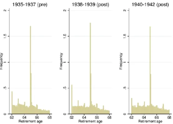
The retirement effects of the reform are perhaps best illustrated in a histogram. Figure 2 shows the retirement distribution for pre- and post-reform cohorts in the treatment group. Most evident in the left-most panel is the spike of retirements around age 63. The spike around 65 is also pronounced, which means that many workers continue to work past the age at which they become entitled to full pension benefits. The two oldest post-reform cohorts, i.e. those born in 1938 and 1939, seem to retire later than the pre-reform cohorts, but the spike around 63 is only marginally smaller. Remarkably, it almost vanishes for the 1940–1942 cohorts. These graphs provide clear evidence that the reform increased the actual retirement age.
Figure 2. Retirement distribution for local government workers (by cohort)
Note: Histogram of retirements in the treatment group. The decision to retire is equated with the month in which the individual's last employer reports the employment contract to be officially ended. See Table 2 for more information on the sample of analysis.
I proceed by presenting first-stage OLS estimates of Equations (2) and (3). The results are presented in Table 4. Column (1) presents the common treatment effect from the just-identified case, while column (2) allows for heterogeneous effects across birth cohorts, i.e. the over-identified case. The common treatment effect amounts to 4.5 months, providing clear evidence that the first assumption of the IV model holds. Column (2) shows that the effect on retirement is largely driven by the youngest cohorts. For example, those born in 1942 retire more than 6.2 months later than the pre-reform cohorts as compared to 1.4 months for those born in 1939.
Table 4. First-stage results (1) (2) (3) Post-reform CH * LG 4.474*** (0.274) Cohort 1942 * LG 6.217*** 5.684*** (0.379) (0.488) Cohort 1941 * LG 5.371*** 4.836*** (0.395) (0.501) Cohort 1940 * LG 5.691*** 5.156*** (0.397) (0.502) Cohort 1939 * LG 1.893*** 1.358*** (0.418) (0.520) Cohort 1938 * LG 2.695*** 2.159*** (0.424) (0.525) Pre-reform cohorts Cohort 1936 * LG -0.603 (0.551) Cohort 1935 * LG -1.057* (0.557) Observations 133,026 133,026 133,026 Mean dep. var. 40.708 40.708 40.708 F-statistic 265.869 81.565 45.792
Note: Column (1) shows first-stage estimates from Equation (2) and columns (2) and (3) from Equation 3. Column (3) adds two pre-reform interaction terms between cohort 𝑗 = (1935, 1936) and the local government dummy to the specification in column (2). Robust standard errors in parentheses. Dependent variable: number of months employed from age 62 to 68. Estimated using OLS. Dependent variable right-censored at 72 (age 68). All regressions include cohort-fixed effects, regional dummies and dummies for month of birth. Additional control variables are the log of the average of yearly earnings between ages 56-60, the log of the standard deviation of yearly earnings between ages 56-60, number of years of schooling, dummies for immigrant status and having children at home, the number of years with more than 14 consecutive days of sick leave between ages 56 and 60, and interactions between schooling years/income and cohort and schooling years/income and local government. ***, **, * denote statistical significance at the 1%, 5% and 10% level respectively. See Table 2 for more information on the sample of analysis.
How can we be sure that this movement in the retirement mass is not only the result of a general trend towards longer working lives? Figure 3 shows retirement distributions for the control group. Except for a slight decrease in the mass of retirements at ages 62 and 63, little seems to happen across these birth cohorts. I also estimate pre-reform trends for the retirement age in a similar fashion as for health in the previous section. Column (3) of Table 4 reports the estimation results after adding two interaction terms between pre-reform cohort j=(1935, 1936) and the local government dummy to the specification in column (2). The estimated coefficients imply that local government workers born in 1935 and 1936 retire 0.5 and 1.1 months earlier than those born in 1937, respectively, accounting for the corresponding change in the control group. The coefficient for the