Modeling and Simulation of Urea Dosing System

(1)

Master Thesis May 2013

Modeling and Simulation of Urea Dosing System

Zaki Ahmed

Supervisors: Johan Wängdahl and Kurre Källkvist, Scania Supervisor: Associate Professor Mattias Dahl, BTH Examiner: Associate Professor Claes Jogrèus, BTH

School of Engineering

Blekinge Institute of Technology SE – 371 79 Karlskrona

(2)

Acknowledgment

Completion of this thesis was possible with the support of several people. I would like to express my sincere gratitude to all of them.

I am extremely grateful to Malin Bard, Head of Engine Mechtronics, NESM department, for her valuable guidance, inputs and consistent encouragement I received throughout the thesis work. I am indebted to many people for making the time working on my thesis unforgettable experience. I am deeply grateful to my industrial supervisors Johan Wängdahl and Kurre Källkvist. To work with you has been a real pleasure to me, full of fun and excitement you have responded to my questions and query so promptly, and have always been patient and encouraging in times of new ideas.

Furthermore, I am very grateful to my university supervisor Associate Professor Mattias Dahl, for insightful comments both in my work and in this thesis, for his support, and for many motivating discussions. I would also like to express my deepest appreciation to Associate Professor Claes Jogrèus for teaching me many skills that will help for my future career.

I take this time to express my gratitude to the Scania’s library staff Iréne Wahlqvist, Anne-Maria Anderssonfor their prompt services.

In addition, I have been very privileged to get to know and have discussions with many great people at the NESM department. I learned a lot from you, practical information about Scania Jörgen Mårdberg has been a pleasure to work with. Your technical depth and attention to model detail, which I experienced during our meetings at the NMTP department. Thank you for teaching me so much about GT Suite software. I have greatly enjoyed the opportunity to learn from you.

(3)

Abstract

To protect our health and environment from pollution, among others regulatory agencies in the European Union (EU) and legislation from the U.S. Environmental Protection Agency (EPA) has required that pollutants produced by diesel engines - such as nitrogen oxides (NOx), hydrocarbons (HC) and particulate matter (PM) - be reduced.

The key emission reduction and control technologies available for NOx control on Diesel engines are combination of Exhaust Gas Recirculation (EGR) and Selective Catalytic Reduction (SCR).

SCR addresses emission reduction through the use of Diesel Exhuast Fluid (DEF), which has a trade-name AdBlue. Which is 32.5% high purity urea and 67.5% deionized water, Adblue in the hot exhaust gas decomposes into ammonia (NH3) which then reacts with surface of the catalyst to produce harmless nitrogen(N2) and water (H20).

Highest NOx conversion ratios while avoiding ammonia slip is achieved by Efficient SCR and accurate Urea Dosing System it’s therefore critical we model and simulate the UDS in order to analyze and gain holistic understanding of the UDS dynamic behavior.

The process of Modeling and Simulating of Urea Dosing System is a result of a compromise between two opposing trends. Firstly, one needs to use as much mathematical models as it takes to correctly describe the fundamental principles of fluid dynamics such as, (1) mass is conserved (2), Newton’s second law and (3) energy is conserved, secondly the model needs to be as simple as possible, in order to express a simple and useful picture of real systems.

Numerical model for the simulation of Urea Dosing System is implemented in GT Suite® environment, it is complete UDS Model (Hydraulic circuit and Dosing Unit) and it stands out for its ease of use and simulation fastness, The UDS model has been developed and validated using as reference Hilite Airless Dosing System at the ATC Lab, results provided by the model allow to analyze the UDS pump operation, as well the complete system, showing the trend of some important parameters which are difficult to measure such as viscosity, density, Reynolds number and giving plenty of useful information to understand the influence of the main design parameters of the pump, such as volumetric efficiency, speed and flow relations.

(4)

Acronyms

The following Abbreviations will be used in this thesis: ASC Ammonium Slip Catalyst DEF Diesel Exhaust Fluid DOC Diesel Oxidation Catalyst DPF Diesel Particulate Filter

EEC Exhaust Emmission Controller EGR Exhaust Gas Recirculation EMS Engine Management System EU European Union

EPA Environmental Protection Agency GT Gamma Technologies

(7)

HC Hydrocarbons

ISO International Organization for Standardization N2 Nitrogen

NH3 Ammonia NOx Nitrogen Oxides

PM Particulate Matter

PWM Pulse Width Modulation RPM Revolution Per Minute SCR Selective Catalytic Reduction UDC Urea Dosing System

VGT Variable Geometry Turbocharger XPI Xtra Pressure Injection

NS Navier Stokes Re Reynolds number RHS Right Hand Side VE Volumetric Efficiency

Nomenclature

m Mass flow rate m Mass

A Cross sectional area Cd Discharge coefficient

D Diameter F Force g Gravity

(8)

L Length of pipe P Pressure

Q Volumetric flow rate

r Radial distance from the centre of pipe S Surface of control volume or pump stroke T Temperature

t Time

𝑢𝑚𝑎𝑥 Maximum velocity

u, v, w Cartesian components of velocity W Pump power

V Volume or velocity x, y, z Cartesian coordinates

(9)

1

1 Introduction

1.1 Background

The modern Diesel engine is one of the most versatile power sources available for mobile applications. The high fuel economy and torque of the Diesel engine has long resulted in global application for heavy-duty applications [1].

However, the demand for Diesel vehicles can only be realized if their exhaust emissions meet the increasingly stringent emissions standards being introduced around the world, below is chart showing progression of European emission standards [2].

(10)

2 1.1.1 Exhaust after-treatment system

Achieving future emissions legislation is a challenge for all engine manufacturers, in order to comply with emission standards engine manufacturers use different technologies and techniques, Selective catalytic reduction (SCR) is a well-established technique to reduce NOx emissions from diesel engines. For stationary applications ammonia can be used as a reductant. For mobile applications the ammonia is generated from an aqueous urea solution, AdBlue, Compared to other technologies, such as exhaust gas recirculation (EGR) and NOx-adsorbers, SCR has shown to better fuel economy since a more advanced timing of the diesel injection can be used. It is often combined with other technologies to meet specifications on both NOx and PM [4]. Scania uses a combination of different technologies as shown in figure 2.

The upstream NOx sensor, diesel oxidation catalyst (DOC), full-flow diesel particulate filter (DPF), AdBlue mixer, twin parallel SCR catalysts, ammonium slip catalyst (ASC) and downstream NOx sensor are all integrated in the compact silencer unit. The temperature (°C) is measured all the way up to the catalysts, and the pressure drop (ΔP) across the DPF is monitored to assess the status of the filter [3].

(11)

3 1.1.2 Urea Dosing System

The UDS is a critical sub-system in Urea-SCR reduction system, it is important to explain system functionality before we start modeling and simulating of the UDS. In this section we will explain Scania’s Airless Dosing System shown below.

Figure 3: Scania’s Urea Dosing System [5]

The supply unit sucks the urea water solution form the tank, pressurizes and filters it and delivers it to the dosing unit. By adapting the motor speed, the pump regulates the system pressure to a constant value of approximately 9-10 bar [6].

The dosing unit gathers the current state of the system doses the required amount of urea and sprays it into the exhaust gas stream [6].

(12)

4

1.2 Purpose

The Goal of this thesis is to implement following three steps:

1.2.1 Modeling and Simulation: we will show simplified representation of UDS to promote understanding of the real system, then we will execute model over time and will observe system behavior by focusing on the following parameters:

Parameters of interest are:

• Line Pressure of 9-10 bar

• Flow rate when no injection 150g/min • Dosing Unit mass flow rate 50g/min

1.2.2 Verification: we will make sure that step 1.2.1 is implemented accurately and specifications that the model was designed to is achieved (e.g. right flow, pressure, and dosing unit mass flow rate)

1.2.3 Validation: we will see the degree to which our model is an accurate representation of the real UDS from the perspective of the practical application of the model

1.3 Delimitation

In This thesis we will model, simulate, verify and validate Urea Dosing System, the model will be validated with real system data, we will also analyze dynamics of selected parameters, the model validation will be limited to with one data set where Adblue injection is 50g/minute.

1.4 Method

We will start with basic physical principles of fluid motion such as conservation of mass, and conservation of moment, we will present incompressible Navier Stokes partial differential equations which link to the problem.

We will derive some simple yet effective mathematical models for circular cross section hoses Hagen-Poiseuille Law, and well known Euler’s and Bernoulli equation, we will use GT suite v7.3.0 , GT suite provides solution to the Navier Stokes equations we mentioned above (such as conservation of mass momentum and energy ) [7] finally will analyze some selected parameters of interest.

(13)

5

2 _Theory

2.1 Modeling of the Flow

The fundamental governing equations of fluid dynamics is to find the velocity field describing the flow in a given domain [8] This section of the thesis we will discuss mathematical equations of the three basic equations of fluid flow, which all fluid dynamics is based [9].

 Conversation of Mass

 Conservation of Momentum

 Conservation of Energy

These fundamental flow principles can be expressed in terms of mathematical equations mainly these equations are partial differential equations [9] in this thesis we will not cover conservation of energy as this is beyond scope of the thesis.

2.2 The continuum hypothesis

In simple terms this says that when dealing with fluids we can ignore the fact that fluid consists of microscopic individual molecules or atoms, and instead we treat the properties of that region as if it were a continuum [10] by applying to this assumption we may treat any fluid property as varying continuously from one point to the next within the fluid; this hypothesis leads us to study of fluid dynamics at macroscopic scale [10][8].

2.3 Conservation of mass

We use the term Conserved which means constant or unchanged. We can therefore say that mass neither is created nor destroyed.

2.3.1 Continuity equation

One of the main principles used in the analysis of uniform flow is known as the Continuity of Flow. This principle is mathematically derived from the fact that regardless of the pipeline complexity or direction of flow mass is conserved in fluid systems

(14)

6

Figure 4: Finite control fixed in space [9]

We can say that rate of decrease of mass in 𝑉 = −𝑑

𝑑𝑡 𝜌_𝑉 𝑑𝑉 = − 𝜌_𝑉 𝜕𝜌

𝜕𝑡𝑑𝑉 (1)

The rate of external mass flux across any small element dS of S is ρ v ・ dS where the magnitude of dS is equal to the element’s area and we take dS along the outward normal. By integrating over the complete surface we have [8] rate of mass flux out of

𝑉 = 𝜌𝐯. 𝑑𝑆 =

𝑆

𝛻・(

𝑉

𝜌𝐯)𝑑 (2)

By applying Green’s formula to convert to a volume integral [8]. The integrand 𝜵・ 𝝆𝒗 on the RHS is can be expressed in Cartesian coordinates x = 𝑥, 𝑦, 𝑧 , and v =(𝑢, 𝑣, 𝑤) as

𝛻・ 𝜌𝑣 =𝜕 𝜌𝑢 𝜕𝑥 + 𝜕 𝜌𝑣 𝜕𝑦 + 𝜕 𝜌𝑤 𝜕𝑧 (3) Equation 3 was written in the Cartesian coordinates system, Cartesian coordinates have fewest numbers of terms and these coordinates are compact compared to the other coordinate systems, for simplicity in this thesis we will only use Cartesian coordinate system.

(15)

7

Figure 5: Mass entering and leaving an element [8]

For mass to be conserved everywhere, Equations 1 and 2 must be equal for any volume V and so we obtain the continuity equation[8].

𝜕𝜌

𝜕𝑡 + 𝛻・ 𝜌𝐯 = 0 (4)

Equation 4 is the local form of the continuity equation different forms of the continuity equation can be found [9][11].

2.3.2 The material derivative

The total rate of change D/DT is called material derivative also substantial or particle derivative where _𝐷𝑡𝐷 ≡_𝜕𝑥𝜕 + 𝑽 ∙ 𝛁. This defines the material (or substantive) derivative, if we say 𝜕𝑓_𝜕𝑡 we might be interested the rate of change of f at particular point that is fixed in space or we might be interested the rate change of f in a given element of fluid as it moves along trajectory where x = x(t) [8].

(16)

8 𝐷𝑓 𝐷𝑡 = 𝑑 𝑑𝑥𝑓 𝑥 𝑡 , 𝑦 𝑡 , 𝑧 𝑡 , 𝑡 = 𝜕𝑓 𝜕𝑡 + 𝑑𝑥 𝑑𝑡 𝜕𝑓 𝜕𝑥+ 𝑑𝑦 𝑑𝑡 𝜕𝑓 𝜕𝑦+ 𝑑𝑧 𝑑𝑡 𝜕𝑓 𝜕𝑧 = 𝜕𝑓 𝜕𝑡+ 𝑢 𝜕𝑓 𝜕𝑥+ 𝑣 𝜕𝑓 𝜕𝑦+ 𝑤 𝜕𝑓 𝜕𝑧 = 𝜕𝑓 𝜕𝑡 + 𝐯・∇𝑓 (5) We can interpret equation 5 that any given element can suffer changes in f (v ・ ∇ f) as it moves from one place to other. Where 𝜕𝑓_𝜕𝑡 = 0 [8] we therefore obtain the continuity equation

𝐷𝜌

𝐷𝑡 + 𝜌∇. v = 0 (6) Which also can be rewritten in the form of

𝜕𝜌

𝜕𝑡 + 𝐯 ∙ ∇𝜌 + 𝜌∇ ∙ 𝐯 = 𝜕𝜌

𝜕𝑡 + ∇ ∙ 𝜌𝐯 = 0 (7)

For simplicity we neglect the compressibility of fluid by saying that ρ = constant, independent of space and time, Thus, the continuity equation for incompressible flow is

∇ ∙ 𝐯 = 0 (8) Which can be written in Cartesian coordinate system

𝜕𝑢 𝜕𝑥 + 𝜕𝑣 𝜕𝑦+ 𝜕𝑤 𝜕𝑧 = 0 (9)

Equation 9 is the continuity equation for incompressible flow whether the flow is steady or unsteady.

(17)

9

2.4 Conservation of moment

To model the flow we apply Newton’s second law, which states that the rate of change of change of momentum of a body is equal to the net force acting on it [13] where m is the mass, V is velocity, and F is sum of the forces acting on it

𝑑

𝑑𝑥 𝑚𝑽 = 𝑭 (10) For a fluid element of unit volume within a flow, left side of the above equation is by the material derivative [13]

𝜌 𝐷

𝐷𝑡𝑉 = 𝜌 𝜕

𝜕𝑥 𝑽 + 𝑽 ∙ ∇ 𝑽 (11) Where V is the velocity of the flow, 𝜌 is the fluid density, ∇ del operator

We can write this in the Cartesian coordinates

𝜌 𝐷𝑢 𝐷𝑡 = 𝜌 𝜕𝑢 𝜕𝑡 + 𝑢 𝜕𝑢 𝜕𝑥+ 𝑣 𝜕𝑢 𝜕𝑦+ 𝑤 𝜕𝑢 𝜕𝑧 𝜌 𝐷𝑣 𝐷𝑡 = 𝜌 𝜕𝑣 𝜕𝑡 + 𝑢 𝜕𝑣 𝜕𝑥+ 𝑣 𝜕𝑣 𝜕𝑦+ 𝑤 𝜕𝑣 𝜕𝑧 (12) 𝜌 𝐷𝑤 𝐷𝑡 = 𝜌 𝜕𝑤 𝜕𝑡 + 𝑢 𝜕𝑤 𝜕𝑥 + 𝑣 𝜕𝑤 𝜕𝑦 + 𝑤 𝜕𝑤 𝜕𝑧

There are two forces acting on the fluid element namely, body forces and surface forces:

 Body forces. they act directly on volumetric mass for the fluid element, such gravity [13][9]

 Surface forces. which are pressure and friction forces [13]

(18)

10 𝑀𝑜𝑚𝑒𝑛𝑡𝑢𝑚, 𝑥: 𝜌 𝐷𝑢 𝐷𝑡 = 𝜌𝑔𝑥+ 𝜕𝜏_𝑥𝑥 𝜕𝑥 + 𝜕𝜏𝑦𝑥 𝜕𝑦 + 𝜕𝜏_𝑧𝑥 𝜕𝑧 𝑀𝑜𝑚𝑒𝑛𝑡𝑢𝑚, 𝑦: 𝜌 𝐷𝑣 𝐷𝑡 = 𝜌𝑔𝑦 + 𝜕𝜏_𝑥𝑦 𝜕𝑥 + 𝜕𝜏_𝑦𝑦 𝜕𝑦 + 𝜕𝜏_𝑧𝑦 𝜕𝑧 (13) 𝑀𝑜𝑚𝑒𝑛𝑡𝑢𝑚, 𝑧: 𝜌 𝐷𝑤 𝐷𝑡 = 𝜌𝑔𝑧 + 𝜕𝜏𝑥𝑧 𝜕𝑥 + 𝜕𝜏_𝑦𝑧 𝜕𝑦 + 𝜕𝜏𝑧𝑧 𝜕𝑧

If the following is not true any small fluid will lead to infinite angular acceleration[8]

𝜏𝑥𝑦 =𝜏𝑦𝑥 , 𝜏𝑧𝑥=𝜏𝑥𝑧 , 𝜏𝑦𝑧 =𝜏𝑧𝑦 (14)

Detailed discussions about the shear and normal stress can be found [9][11][13][14]

𝝉ij is the force per unit area in the i direction across a plane with normal in the j direction[8] normal stress is denoted by 𝝉_𝒙𝒙 and shear stress is denoted by 𝝉_𝒙𝒚 [9].

2.4.1 Constitutive relations

The surface stresses [𝝉𝒊𝒋] on any element arise from a combination of pressure p and viscous

friction, as shown by the constitutive relations [8]. 𝜏𝑥𝑥 = − 𝑝 + 𝜆𝛻 ∙ 𝑉 + 2𝜇 𝜕𝑢 𝜕𝑥, 𝜏𝑥𝑦 = 𝜇 𝜕𝑢 𝜕𝑦+ 𝜕𝑣 𝜕𝑥 (15) 𝜏𝑦𝑦 = − 𝑝 + 𝜆𝛻 ∙ 𝑉 + 2𝜇 𝜕𝑣 𝜕𝑦, 𝜏𝑦𝑧 = 𝜇 𝜕𝑣 𝜕𝑧+ 𝜕𝑤 𝜕𝑦 (16) 𝜏_𝑧𝑧= − 𝑝 + 𝜆𝛻 ∙ 𝑉 + 2𝜇𝜕𝑤 𝜕𝑧, 𝜏𝑥𝑧 = 𝜇 𝜕𝑢 𝜕𝑧+ 𝜕𝑤 𝜕𝑥 (17) Where 𝝁 is the coefficient of dynamic viscosity and 𝝀 is a coefficient of bulk viscosity, in these equations relationship between stress and velocity is linear and isotropic.

(19)

11 2.4.2 Navier-Stokes equations

Relationship between pressure, density, velocity and temperature of a fluid flow is well expressed by the Navier-Stokes equations, these equations are extension of Euler’s equations and cover flow viscosity, theses equations are partial differential equations and are very difficult to solve analytically, here we will discuss incompressible flow where we already know that constant density will lead us to Equation 9 where 𝛁 ∙ 𝑽 = 𝟎, incompressible fluid model will be quite accurate approximation where the velocity is much smaller than speed.

Kronecker’s delta cases 𝛿𝑖𝑗 = _{0 𝑖𝑓 𝑖 ≠ 𝑗}1 𝑖𝑓 𝑖 = 𝑗

Constitutive relations becomes

𝜏_{𝑖𝑗 =}− 𝑝 𝛿_𝑖𝑗 + 𝜇 𝜕𝑢𝑖 𝜕𝑥𝑗 +

𝜕𝑢_𝑗

𝜕𝑥𝑗 (18)

To get into the Navier-Stokes equations we have to make some assumptions such as, incompressible flow 𝛁 ∙ 𝑽 = 𝟎, constantant density 𝜌, and constant viscosity

𝜇

and this will lead us to the incompressible Navier-Stokes equations, detailed disucssions of the Naveir-Stokes equations can be found [9] and [11]

Continuity equation is 0 =𝜕𝑢 𝜕𝑥+ 𝜕𝑣 𝜕𝑦+ 𝜕𝑤 𝜕𝑧 𝑀𝑜𝑚𝑒𝑛𝑡𝑢𝑚, 𝑥: 𝜌 𝐷𝑢 𝐷𝑡 = 𝜌𝑔𝑥− 𝜕𝑝 𝜕𝑥+ 𝜇 𝜕2_𝑢 𝜕𝑥2 + 𝜕2_𝑢 𝜕𝑦2 + 𝜕2_𝑢 𝜕𝑧2 𝑀𝑜𝑚𝑒𝑛𝑡𝑢𝑚, 𝑦: 𝜌 𝐷𝑣 𝐷𝑡 = 𝜌𝑔𝑦 − 𝜕𝑝 𝜕𝑦+ 𝜇 𝜕2_𝑣 𝜕𝑥2 + 𝜕2_𝑣 𝜕𝑦2+ 𝜕2_𝑣 𝜕𝑧2 𝑀𝑜𝑚𝑒𝑛𝑡𝑢𝑚, 𝑧: 𝜌 𝐷𝑤 𝐷𝑡 = 𝜌𝑔𝑧 − 𝜕𝑝 𝜕𝑧+ 𝜇 𝜕2_𝑤 𝜕𝑥2 + 𝜕2_𝑤 𝜕𝑦2 + 𝜕2_𝑤 𝜕𝑧2 (19)

(20)

12

Continuity: ∇ ∙ 𝑉 = 0 (20)

𝑀𝑜𝑚𝑒𝑛𝑡𝑢𝑚: 𝜌 𝐷𝑉

𝐷𝑡 = 𝜌𝑔 − ∇𝑝 + 𝜇∆V (21) In this section, we have seen the basic governing equations incompressible fluid flow, to derive Euler’s equations later, will show flow fields that are time-independent and two dimensional in Cartesian coordinates (x, y) , as shown here

Continuity 𝜕𝑢 𝜕𝑥+ 𝜕𝑣 𝜕𝑦 = 0 (22) Momentum 𝜌 𝑢𝜕𝑢 𝜕𝑥+ 𝑣 𝜕𝑢 𝜕𝑦 = − 𝜕𝑃 𝜕𝑥+ 𝜇 𝜕2_𝑢 𝜕𝑥2 + 𝜕2_𝑢 𝜕𝑦2 (23) 𝜌 𝑢𝜕𝑣 𝜕𝑥+ 𝑣 𝜕𝑣 𝜕𝑦 = − 𝜕𝑃 𝜕𝑦+ 𝜇 𝜕2_𝑣 𝜕𝑥2 + 𝜕2_𝑣 𝜕𝑦2 (24)

2.5 Poiseuille Flow

Since Urea Dosing System has pressure-driven flow in circular cross section hoses it is important to have mathematical model that can express the relationship between the pressure gradient in the hose, flow rate in the hose, diameter of the hose, length of the hose and viscosity of the liquid, the model which describes all these relations is called Hagen-Poiseille model which will be derived here with some assumptions.

2.5.1 Hagen-Poiseuille Law

To derive Hagen-Poiseuille equation we will make some assumptions as:

 Laminar flow  Constant viscosity  Straight pipe 𝑝1− 𝑝2 = 8𝜇𝑉 𝑟₀2 𝐿 = 32𝜇𝑉 𝐷2 𝐿 (25)

(21)

13

All disciplines of engineering are based on sets of fundamental laws or relations, Eelectrical engineering relies on Kirchhoff’s laws, mechanical engineering on Newton’s law, electromagnetic on Faraday’s and Lenz law, fluid on continuity and Bernoulli’s law, these laws are to predict behavior of system [15], alternatively one can use model by analogy in order to model the UDS pump and hydraulic hoses this research has been by done [16][17][18] and supplementary reading can be found [19][20]

2.6 Euler’s Equations

The following is two- dimensional and time-independent equations

𝑀𝑜𝑚𝑒𝑛𝑡𝑢𝑚 ∶ 𝜌 𝑢𝜕𝑢 𝜕𝑥+ 𝑣 𝜕𝑢 𝜕𝑦 = − 𝜕𝑃 𝜕𝑥+ 𝜇 𝜕2_𝑢 𝜕𝑥2 + 𝜕2_𝑢 𝜕𝑦2

Neglecting the viscosity of the fluid by making 𝜇 = 0, we will get the Euler equations of two-dimensional 𝑀𝑜𝑚𝑒𝑛𝑡𝑢𝑚 𝑥 ∶ −1 𝑝 𝜕𝑝 𝜕𝑥= 𝑢 𝜕𝑢 𝜕𝑥+ 𝑤 𝜕𝑢 𝜕𝑧 (26) 𝑀𝑜𝑚𝑒𝑛𝑡𝑢𝑚 𝑧 ∶ −1 𝑝 𝜕𝑝 𝜕𝑧= 𝑢 𝜕𝑤 𝜕𝑥 + 𝑤 𝜕𝑤 𝜕𝑧 + 𝑔 (27) And two-dimensional continuity equation is

𝜕𝑢 𝜕𝑥+

𝜕𝑤

𝜕𝑧 = 0 ( 28) The Euler equations are simultaneous partial differential equations that are basic to the solution of two-dimensional flow field problems[21]; solution of these equations yields p, u and w as functions of x and z, we can predict the pressure and velocity at any point in the flow field [21]. Further explanations is available at Atil’s lecture notes [21][23].

As we have seen above Euler equations neglect the viscosity of the fluid which were included in the incompressible Navier-Stokes equations, solution of Euler equations is therefore only approximations to real fluids problems, might be a good model for the thin airfoil, other problems Euler equations do not model the problem accurately [22].

(22)

14

2.7 Bernouli’s Equation

Bernoulli’s equation will be derived by Integrating Euler equations for constant 𝑑𝑒𝑛𝑠𝑖𝑡𝑦 𝜌 23 derivation of the Bernouli equation is shown at appendix E.

By assuming steady-state, incompressible (constant density), in viscid, laminar flow in a horizontal pipe (no change in height) with negligible frictional losses, Bernoulli's equation reduces to an equation relating the conservation of energy between two points on the same streamline, influence of the heights in Bernoulli’s equation is negligible[21].

Bernoulli equation assumptions might have plenty of assumptions, however these equations give great insight about relations between pressure, velocity and elevation

𝑉12 2𝑔+ 𝑝1 𝛾 + 𝑧1 = 𝑉₂2 2𝑔+ 𝑝2 𝛾 + 𝑧2 (29) 𝑉𝑒𝑙𝑜𝑐𝑖𝑡𝑦 𝑕𝑒𝑎𝑑 ∶ 𝑉1 2 2𝑔 𝑃𝑟𝑒𝑠𝑠𝑢𝑟𝑒 𝑕𝑒𝑎𝑑 ∶ 𝑝1 𝛾 𝑒𝑙𝑒𝑣𝑎𝑡𝑖𝑜𝑛 𝑕𝑒𝑎𝑑 ∶ 𝑧 Potential energy of fluid is .

𝛾 = 𝜌𝑔

2.8 Reynolds number

By using incompressible Navier-Stokes equations we can derive Reynolds number

𝑀𝑜𝑚𝑒𝑛𝑡𝑢𝑚: 𝜌 𝐷𝑉

(23)

15

To make the above equation non-dimensional equation, we will multiply by the factor _𝜌𝑉 𝐷₂ v is the mean velocity, D is the diameter, and 𝝆 fluid density [24][31]

If we now set: 𝑣′ ₌ 𝑣 𝑉 , 𝑝′ = 𝑝 1 𝜌𝑉2 , 𝑓′ = 𝑓 𝐷 𝜌𝑉2 , 𝜕 𝜕𝑡′ = 𝐷 𝑉 𝜕 𝜕𝑡 , ∇′= 𝐷∇

We can rewrite the Navier-Stokes equation without dimensions 𝐷𝑉′

𝐷𝑡′ = 𝑓′ − ∇′𝑝′+

𝜇 𝜌𝐷𝑉 ∆′V′ To make it easy we omit the primes

𝐷𝑉 𝐷𝑡 = 𝑓 − ∇𝑝 + 1 𝑅𝑒 ∆V Where 𝜇 𝜌𝐷𝑉= 1 𝑅𝑒 𝑅𝑒 = 𝜌𝐷𝑉 𝜇 = 𝐼𝑛𝑒𝑟𝑡𝑖𝑎𝑙 𝑓𝑜𝑟𝑐𝑒 𝑉𝑖𝑠𝑐𝑜𝑢𝑠 𝑓𝑜𝑟𝑐𝑒 If 𝑅 → ∞ the viscous terms vanish

Flow in circular pipe

𝑅𝑒 =𝜌𝐷𝑉 𝜇 = 𝐷𝑉 𝑣 (30)

Where Re is called Reynolds number, ρ is the fluid density, V is the fluid velocity, D is the pipe diameter, µ is the fluid dynamic viscosity and ν is the of the fluid kinematic viscosity [24]

(24)

16 2.8.1 Significance of Reynolds’s Number

Re less than 2000 indicates that flow is laminar. If Re is between 2000 and 4000, it shows a transitional flow and Re greater than 4000 indicates turbulent flow

As shown above Reynolds number gives the ratio between inertial forces and viscous forces in other words we can estimate which forces are dominant, whether we have laminar, translational or turbulent.

Until now we have completed the mathematical representation of the fluid model, The Navier-Stokes equations consists of a time-dependent continuity equation for conservation of mass, three time-dependent conservation of momentum equations and a time-dependent conservation of energy equation.

There are four independent variables in the problem, the x, y, and z spatial coordinates of some domain, and the time t. There are six dependent variables; the pressure p, density r, and temperature T (which is contained in the energy equation) and three components of the velocity vector; the v component is in the x direction, the v component is in the y direction, and the w component is in the z direction, All of the dependent variables are functions of all four independent variables. The differential equations are therefore partial differential equations and not the ordinary differential equations [22] We can say that analytical solutions of the Navier-Stokes equations is not possible.[19].

(25)

17

3 Model Development

3.1 Model calibration

In the Model development section we will implement first and second step of the goal statement, to make the model calibration easier the systems has been dived into the following section:

 Hydraulic circuit (Supply unit)

 Dosing unit

3.1.1 Hydraulic circuit model calibration

Hydraulic circuit consists of a suction hose, two filters to remove dirt particles from the Adblue liquid, Dc motor, positive displacement pump, and pressure relieve valve as shown below

3.1.1.1 Hydraulic circuit model simplification

Under normal operation the pressure relieve valve is closed and does effect the system dynamics, therefore pressure relieve is not modeled.

Since we have divided the systems into two sections and simplified, we will be calibrating hydraulic circuit, firstly we run the hydraulic circuit at steady-state with no injection to isolate calibration of pump and orifice, running at 1050 rpm since that is the speed we have in the real system data when there is no injection. In this situation, the system pressure is simply a function of the pump outlet flow rate (displacement, volumetric efficiency, and speed) and the outlet orifice size (diameter and discharge coefficient).

(26)

18

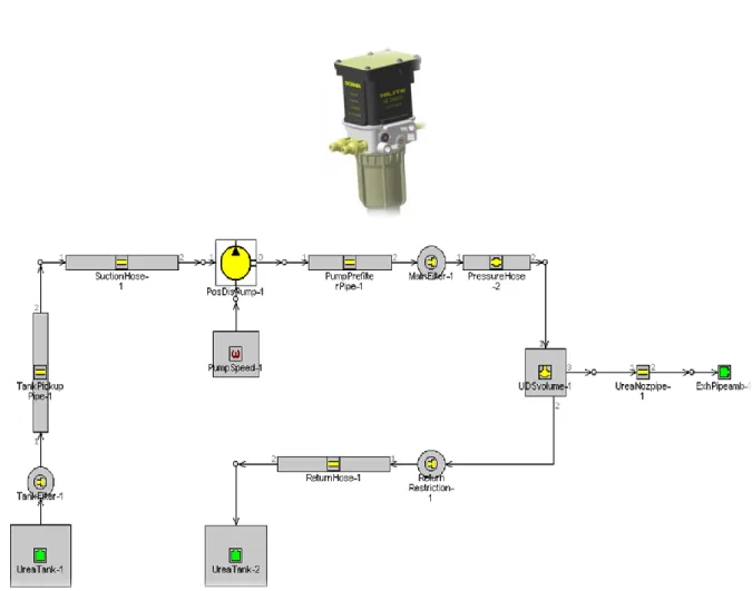
Figure 6: Hydraulic circuit [6]

3.2 GT-Suite model of hydraulic circuit

The hydraulic circuit consists of a urea tank, tank pick-up pipe, suction hose, dc motor, positive displacement pump, pre-filter pipe, main filter, pressure hose, UDS volume, return restriction or Throttle and return hose.

3.2.1 Positive Displacement Pump Model

This object is used to model a positive displacement pump, where the flow rate is more or less linearly proportional to the speed of the pump [25] the pump model has the following equations:

Displacement per Revolution The ideal displacement of the pump per revolution, ignoring the

(27)

19

𝐷𝑖𝑠𝑝𝑙𝑎𝑐𝑒𝑚𝑒𝑛𝑡 𝑝𝑒𝑟 𝑟𝑒𝑣𝑜𝑙𝑢𝑡𝑖𝑜𝑛 = 𝐴𝑆 Where A is the cross sectional area and S pump stroke.

The Volumetric Efficiency of the pump. This value will be used to calculate the real flow rate

out of the pump, Q, using the equation below[25]. 𝑄 = 𝜔𝐷𝜂_𝑣𝑜𝑙

Where ω represents the pump speed, D represents the pump Displacement per Revolution, and ηvol represents the Volumetric Efficiency [25].

Total (Isentropic) Efficiency the total efficiency of the pump. This value will be used to

calculate the power required to drive the pump. The relation used for the pump power, W, is

𝑊 = ∆𝑃𝑚

𝜌𝜂_𝑣𝑜𝑙

Where ΔP represents the static pressure rise between the inlet and outlet of the pump, ρ represents the density at the inlet, ṁ represents the mass flow rate through the pump, and ηtotal represents the pump Total (Isentropic) Efficiency [25].

3.2.2 Motor Model

Imposed Speed A constant value or the name of a dependency reference object specifying the

rotational speed [25] here we will use either imposed speed or dependency reference

Initial Angular Position Initial angle of the speed boundary at the start of simulation in our case

this was set to (“def”).

3.2.3 Pipes and Hoses Model

Round Pipe object is used to model pipes such as Tank Pick up pipe, Suction Hose Pump, Pre filter Pipe, Urea Nozzle Pipe, and Return Hose, in this thesis all the pipes and hoses have a round cross-section.

3.2.4 Filters and Return Restriction Pipe Model

Filters and restriction return pipe(throttle) was modeled by using “OrificConn” object which describes an orifice placed between flow components. 'OrificeConn' connects flow components [25].

(28)

20 3.2.5 Exhaust Pipe Ambient Model

Exhaust Pipe Ambient was modeled as “EndEnvironment” object describes end environment boundary conditions of pressure, temperature, and composition [25].

3.2.6 UDS Volume Model

Spherical Flow Split object is used to model fluid volume and connected to Pressure hose, Urea Nozzle pipe, and Return restriction pipe (throttle).

Figure 7: Pump, motor unit and main filter integrated into one unit (top) and GT-Suite hydraulic circuit model

(29)

21

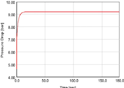
Figure 8: Hydraulic circuit line pressure

From above we can see that the model matches specifications such 9 –10 bar as shown, The objective of sub-systems model calibration was to ensure that the implementation of the model is correct.

3.3 Dosing unit model calibration

Dosing unit consists of pressure hose, dosing valve, throttle which manages the fluid flow by constriction and backflow hose as shown below and a filter.

3.3.1 Dosing unit model simplification

We start with calibrating the dosing unit to get the right mass flow rate. So in sections 3.1-3.2, we can see that we calibrate each part of the system separately. If we have problems with either, it is much easier to pinpoint or identify the problem. We integrate the two calibrated and verified sub-systems in to a single model and finally we validate the complete model.

(30)

22

Figure 9: Dosing unit [6]

3.4 GT-Suite model of Dosing Unit

Dosing unit consists of Signal Generator, Mathematic Equation, Pulse Width Modulator and Gain block. Application of each block is available at GT-Suite template library [25].

Dosing unit receives the requested amount of Adblue to inject from the Engine Management System(EMS) unit and calculates a corresponding opening time for the dosing unit, here will use signal generator to act as EMS to request amount of Adblue to be dosed, the signal generator will generate square wave form which will be fed into the math operation block, the math operation object or the block uses the following expression to calculate the output signal which is the duty cycle, (Math operation block, PWM block and Gain block stand for the EEC3)

𝐷𝑢𝑡𝑦 𝑐𝑦𝑐𝑙𝑒 = 𝐴𝑑𝑏𝑙𝑢𝑒

195 100%

The above equation has one variable Adblue which is the amount of Adblue to be dosed and constant value 195 which is the maximum allowable dosing we can therefore calculate the duty cycle for 50g/min as

𝐷𝑢𝑡𝑦 𝑐𝑦𝑐𝑙𝑒 = 50

(31)

23

25 % duty cycle is the percentage of time that pulse is in the ON state as a fraction of the total time then this if fed to a Pulse Width Modulator (PWM) object to produce an output signal that is ON 25% and OFF 75% of the time (1 sec) which is named Dosing PWM , Gain block was used to act as the dosing unit hole with diameter of 0.4mm below is the complete dosing unit model.

(32)

24

Figure 11: Duty cycle for 50g/min

The injection volume is defined by the opening time of the valve. The valve opens once every second. The duration of the “open time” defines the percentage of the maximum flow which is injected at that specific cycle. Typical values for opening duty cycles lie somewhere between (2) 5-95 (100)% [6], for 50g/min duty cycle is 25% which is shown above figure

(33)

25

4 Model Validation

4.1 Complete UDS model validation

In the Model Validation section we would implement third step of the goal statement to determine the degree to which our model is an accurate representation of the real UDS from the perspective of the intended use of the model[26].

Validation data was collected from various sensors of the UDS, the collected data is available at appendix G.

(34)

26 4.1.1 Pump speed

When you look at the motor speed in the experimental data at appendix G you should notice that the pump speed is 3500 rpm for less than 5 seconds, then pump speed drops off to steady speed of 1050 rpm, as soon as the dosing starts the pump speed goes up to 1500 rpm and stays that speed while the system is dosing, as soon as dosing stops the pump speed goes back to steady speed of 1050 rpm, we can deduce from above statement that the real system does not use constant speed.

To accurately model and have the model behave the same way as the real system we have applied the same real pump speed data into the model, the real system pump speed signal is shown here.

(35)

27 4.1.2 Requested Adblue injection

EEC3 is the control unit of the SCR-system and receives the requested amount of Adblue to be injected from the EMS-unit and calculates opening time of the Dosing Unit [5]. The Requested Adblue injection signal from the Signal Generator is shown below

Figure 14: Requested Adblue Injection

4.2 Pump pressure validation

When the diaphragm moves up the volume of pump chamber is increased, the pressure decreases and we have 1 bar at the inlet and we call this suction mode, where Adblue is drawn into the chamber. When the diaphragm moves down the pump chamber pressure increases from decreased volume, the Adblue previously drawn in is forced out with high pressure of 9-10 bar we call this discharge mode, so we have two modes suction mode with low pressure and discharge mode with high pressure from this we can deduce that all our analysis will focus on the high pressure side of the pump [27].

(36)

28

Figure 15: Inlet and outlet pump pressure

From the above figure you can see that the pump creates lower pressure (1 bar) at the inlet so that Adblue can enter, and creates high pressure (10 bar) at the discharge to force Adblue at the outlet, this indicates that the pump is operating according to specification given at the goal statement.

4.3 Flow rate validation

We would decide whether or not the model has resulted in acceptable agreement with the real system data, here we assess.

(37)

29

Figure 16: Flow rate validation

Form the above figure we can see that the pump has virtually constant flow except during injection of urea, where the flow increases from 126g/min to 170g/min and is independent of the system pressure, simulation flow rate is 126 g/min and UDS average flow rate is 150 g/min.

(38)

30

4.3 Dosing Unit Mass flow rate validation

Figure 17: UDS mass flow rate vs. Simulation mass flow rate

From the above Figure Dosing Unit vs. Simulation, where UDS Mass flow Rate is 50g/min and Simulation is 48g/min, You may see that the simulation (blue lines) has thin rectangular pulses, these pulses are the PWM pulses which has 25% Duty cycle and period of 1 second.

(39)

31

4.4 Line pressure validation

Figure 18: UDS vs Simulation

In Figure 18 The model pressure oscillations is not the same as the UDS pressure oscillations, the pressure oscillations may be better modeled by using a higher discharge coefficient on the simple nozzle model, it may also be necessary to model a more complete injector. It therefore such suggested that to use a GTI compound template such as 'HoleTypeInj

(40)

32

5 Results and Discussions

5.1 System parameter analysis

In the model validation section UDS model has resulted acceptable agreement with real system and as a result the model is sufficient for its intended use of system parameter analysis [26] here we will analyze some important parameters and discuss the results

5.1.1 Volumetric efficiency

Volumetric efficiency of the positive displacement pump is calculated as: Volumetric Efficiency (VE) = _{Theoritcal flow}Actual Flow 100

Here we will vary the VE and observe the effect of the VE has on the pressure of the UDS, measurement was taken from pressure hose of the model

Figure 19: Effect of the pressure on the variation of the Volumetric Efficiency

Form the above figure it is evident that pressure of the pump can vary significantly with Volumetric Efficiency , particularly with a low fluid viscosity, such as that of urea.

(41)

33

Figure 20: Mass flow rate as function of Volumetric Efficiency

The above shows the mass flow rate as function of the Volumetric Efficiency, we can therefore say that the system Mass flow rate is simply a function VE, when all the other parameters is held constant.

5.1.2 Return restriction pipe diameter variation

As small particles or dirt accumulate on the main filter media, As a result of that flow is restricted and pressure rises. When the pressure rises above to a level specified by the hose manufacturer, this may result hose burst, Blockage of the UDS return restriction pipe is simulated, this is done by varying return restriction hole diameter as shown in figure 21

(42)

34

Figure 21: Return restriction pipe diameter variation The system pressure variation as results of return restriction diameter variation

5.1.3 Flow rate as function of speed

The flow rate of UDS pump varies proportionally with pump speed as shown in figure 22

(43)

35

Figure 22: flow rate as function of speed

The above figure shows the relationship between the pump speed and the flow rate. From the motor speed we can estimates the flow rate.

5.1.4 Effects of the pipe diameter on the flow pattern

Reynolds number gives the ratio between inertial forces and viscous forces in other words we can estimate which forces are dominant, whether we have laminar, translational or turbulent flow in the UDS, we will observe effects of the pipe diameter on the flow pattern by varying return restriction pipe diameter and keeping all other variables constant.

(44)

36

Figure 23: Effects of the pipe diameter on the flow pattern

From above we can see that the Re is proportional to the pipe diameter as we increase the pipe diameter so will Re, Re is way below 2000 which indicates that flow is laminar

5.1.5 Adblue density

Density of material is its mass per unit volume, in general, density can be changed by changing either the pressure or the temperature. Increasing the pressure always increases the density of a material. Increasing the temperature generally decreases the density, we should note that there are exceptions in this generalization [28].

(45)

37

Figure 24: Adblue density as function of pressure and temperature

The chart above shows density of Adblue as function of pressure and temperature as required by the conservation equation we should note that effect of pressure and temperature of liquid is very small, we can therefore say that the Adblue has constant density.

5.1.6 Adblue Viscosity

Viscosity is a measure of a fluid's resistance to flow. It describes the internal friction of a moving fluid. A fluid with large viscosity resists motion because its molecular makeup gives it a lot of internal friction. A fluid with low viscosity such as Adblue flows easily because its molecular makeup results in very little friction when it is in motion [29].

5.1.6.1 Types of viscosity

There are two ways to express fluid’s viscosity, it can be either expressed as Dynamic viscosity which is also known as absolute viscosity and Kinematic viscosity which is obtained by liquid’s Dynamic viscosity divided by liquid’s density [30]. Adblue Viscosity in different temperatures is shown in the figures below.

(46)

38

Figure 25: Adblue Dynamic Viscosity behavior on different temperature

(47)

39

From above we can see that Adblue viscosity varies with temperature as the Adblue temperature increases its viscosity decreases [30] Detailed Adblue fluid property is shown in Appendix B

5.2 Conclusions

In the theory section, we have shown two fundamental principles of fluid flow, conservation of mass (continuity equation) and conservation of momentum (the Cauchy equation) of fluid motion.

To get to Euler equations we employed the Navier-Stokes equations for incompressible flow, by neglecting fluid viscosity making 𝜇 = 0 [21], with this assumption Navier-Stokes equations take the form of Euler equations, detailed discussions and derivations might be found at Atil’s lecture notes[21][23]

The second last step is derivation of exact solutions to the Navier-Stokes quations, the Hagen– Poiseuille eqautions, by applying basic physics with the assumptions of laminar flow, constant viscosity and straight pipe with circular cross-section, we derived Hagen–Poiseuille eqautions, this led to a relationship between pressure changes over a length L of pipe, and a friction factor associated with viscous effects

We then applied Euler equations to derive well known Bernoulli equation, which signifies that when the velocity increases in a fluid stream, the pressure decreases and when velocity decreases the pressure increases [31] [15]

We must highlight that all of these equations have their roots in the Navier–Stokes equations, once again underscoring the universality of these equations in the context of describing the motion of fluids [10]

Why did we have to derive all these equations? It is important when applying any equation that we are aware of the restrictions on its use, the restrictions are normally seen in the derivation of the equation when certain simplifying assumptions about the nature of the problem are made. If we ignore the restrictions, we may get inaccurate results from the equation. e.g. an equation was derived while assuming that the flow was incompressible, which means that the speed of the flow is much less than the speed of sound. If you use this form for a supersonic flow, the answer will be wrong [32]

In the Modeling and simulations section, the following steps have been completed as given on the goal statement:

 To broaden our level of understanding and interactions of different components we shown simplified model of the UDS

 To ensure model meets requirements and fulfills its intended use we have verified (e.g. Right flow, pressure, and mass flow rate)

 To gain confidence in the model we have validated by comparing model with the real system data and found acceptable agreement

(48)

40

We have also shown Effects of various parameters of the system, such as Volumetric Efficiency of the pump, return restriction diameter variations, relationship between flow rate and speed Finally we have demonstrated Adblue density as function of pressure and temperature, and effects of the temperature on Dynamic and Kinematic viscosity of the Adblue, more Adblue fluid properties is also given on Appendix B

5.3 Future works

Future work may include the following steps

 Model to be expanded to include GTI compound template such as 'HoleTypeInj instead of simple orifice as we have done, then pressure oscillations may be modeled accurately by using complete injector

 Effects of Young Modules in the pressure hoses to be demonstrated

 Validation of the model with range of operating conditions

We also Re is high (>2100), inertial forces dominate viscous forces and the flow is turbulent; if Re number is low (<1100), viscous

s dominate and the flow

is laminar. It is named after thee is high (>2100), inertial forces dominate viscous forces and the flow is turbulent; if Re number is low (<1100), viscous forces dominate and the flow is laminar

(49)

41

References

[1] Walke, P.V., Deshpande, N. V., Kongre, S.C., (2011). Cat-trap exhaust after treatment system for diesel engine. Retrieved February 8, 2013, from

http://www.academicjournals.org/jmer/PDF/Pdf2011/April/Walke%20et%20al.pdf

[2] European emission standards. (2013, January 3). In Wikipedia, the free encyclopedia. Retrieved March 5, 2013, from http://en.wikipedia.org/wiki/European_emission_standards

[3] Scania. (2012). Scania Euro 6, Södertälje, Author.

[4] Majewski, W. A. (2005). SCR Systems for Mobile Engines. Retrieved November 8, 2013, from http://www.dieselnet.com/tech/cat_scr_mobile.php

[5] Scania. (2010). SCR2_UDS; Installation Guideline for UDS (HiLite) subsystem, Södertälje, Author.

[6] Hilite International, Inc. (2010). Installation Guideline Modular Liquid Only SCR System. Marktheidenfeld, Author.

[7] Applications. (n.d.). Gamma Technologies - Engine and Vehicle simulation.

Retrieved December 5, 2012, from

http://www.gtisoft.com/applications/a_Fuel_Injection.php

[8] Tritton, D. J. (1988). Physical fluid dynamics. Oxford: Clarendon Press.

[9] Wendt, J. F., Anderson, J. D., & Von Karman Institute for Fluid Dynamics. (2009). Computational fluid dynamics: An introduction. Berlin: Springer

[10] McDonough, J. M. (2009). Lectures in elementary fluid dynamics. Retrieved March 14, 2013, from http://www.engr.uky.edu/~acfd/me330-lctrs.pdf

[11] Graebel, W.P. (2007). Advanced Fluid Mechanics. Burlington, MA: Academic Press. [12] Kundu, P. K., & Cohen, I. M. (2008). Fluid mechanics. Amsterdam: Academic Press. [13] Zikanov, O. (2010). Essential Computational Fluid Dynamics, Hoboken, N.J: Wiley.

[14] Pozrikidis, C. (2009). Fluid Dynamics: Theory, computation and numerical simulation, New York: Springer.

[15] Bernoulli's Equation. (2009, April 9). Retrieved January 3, 2013, from

http://www.grc.nasa.gov/WWW/k-12/airplane/bern.html

[16] Bourouina, T., Grandchamp, J.P., (1996). Modeling micropumps with electrical equivalent networks, Journal of Micromechanics and Microengineering, 6(1996), 398-404.

(50)

42

[17] Hsu, Y.C., Le, N.B., (2008). Inertial effects on flow rate spectrum of diffuser micropumps, Journal of Biomedical Microdevices 10(2008), 681–692.

[18] Oosterbroek, R.E. (1999). Modeling, design and realization of microfluidic components.

Ph.D. thesis, University of Twente, Enschede, The Netherlands.

[19] Bruus, H. (2008). Theoretical Microfluidics. Oxford: Oxford University Press.

[20] Kirby, B. (2010). Micro-and nanoscale fluid mechanics: Transport in microfluidic devices: New York: Cambridge University Press.

[21] Bulu, A.(n.d.). Lectures notes in fluid mechanics. Retrieved March 14, 2013, from

http://personals.okan.edu.tr/atil.bulu/fluid_mechanics_files/lecture_notes_04.pdf

[22] Navier-Stokes Equations. (2012, April 16). Retrieved January 3, 2013, from

http://www.grc.nasa.gov/WWW/k-12/airplane/nseqs.html

http://personals.okan.edu.tr/atil.bulu/fluid_mechanics_files/lecture_notes_06.pdf

[24] Reynolds number. (2013, January 3). In Wikipedia, the free encyclopedia. Retrieved March 5,2013, from http://en.wikipedia.org/wiki/Reynolds_number

[25] Gamma Technolgies. (2012). G-Suite Template library v7.3.0. Westmont, IL, Author. [26] Thacker, B.H., Doebling, S.W., Hemez, F.M., Anderson, M.C., Pepin, J.E., Rodriguez,

E.A. (2004). Concepts of model verification and validation. Retrieved March 5, 2013, from

http://www.ltas-vis.ulg.ac.be/cmsms/uploads/File/LosAlamos_VerificationValidation.pdf

[27] Diaphragm pump. (2013, February 22). In Wikipedia, the free encyclopedia. Retrieved February 26, 2013, from http://en.wikipedia.org/wiki/Orifice_plate

[28] Denisty. (2013, February 13). In Wikipedia, the free encyclopedia. Retrieved March 1, 2013, from http://en.wikipedia.org/wiki/Density

[29] Definition of viscosity. (n.d.). Retrieved March 14, 2013, from

http://www.princeton.edu/~gasdyn/Research/T-C_Research_Folder/Viscosity_def.html

[30] What is the difference between dynamic and kinematic viscosity? (n.d.). Retrieved January 23, 2013, from http://www.wisegeek.com/what-is-the-difference-between-dynamic-and-kinematic-viscosity.htm

[31] Acheson, D. J. (1990). Elementary fluid dynamics. Oxford: Clarendon Press

[32] Bernoulli's Equation. (2009, April 9). Retrieved January 3, 2013, from

(51)

43

[33] Bernoulli's principle. (2012, January 3). In Wikipedia, the free encyclopedia. Retrieved January 9, 2013, from http://en.wikipedia.org/wiki/Bernoulli's_principle

[34] Orifice plate. (2013, February 13). In Wikipedia, the free encyclopedia. Retrieved January 1, 2013, from http://en.wikipedia.org/wiki/Orifice_plate

http://www.limat.org/data/Handouts/CIVIL/FMbyBulu/lecture_notes_07.pdf

[36] e-nav. (n.d.). Retrieved March 19, 2013 from

(52)

Appendix A

(53)

Appendix B

(54)

(55)

(56)

(57)

Appendix C UDS Pipe view

(58)

Appendix D

Poissoulle equation derivation

Balance of forces [35] 𝒑𝝅𝒓𝟐_{− 𝒑 +}𝝏𝑷

𝝏𝒙𝒅𝒙 𝝅𝒓𝟐− 𝝉 𝟐𝝅𝒓 𝒅𝒙 = 𝟎

The above equations shows the force balance of the momentum equation, where flow is steady Simplifying the above equation we get

𝝉 = −𝝏𝒑 𝝏𝒙

𝒓 𝟐

The ∂p/∂x is called pressure gradient and is x dependent where the flow is laminar. The negative sign shows fluid pressure drop in the direction of flow in a straight pipe, As there is no shearing stress at the center of pipe r=0 and increase linearly with the distance r from the center, reaching its maximum value, where τ0 = (-∂p/∂x) (r0/2), at the pipe wall (r=r0) [35]

Newton’s second law of viscosity states that

(59)

In accordance with the first assumption, τ equals μ(∂u/∂y). Since y equals r0-r, it follows ∂y

equals -∂r. we can therefore say that [35]

𝝉 = −𝝁𝝏𝒖

𝝏𝒓

Where the negative sign indicates shear stress, and is from a region of higher velocity to lower velocity, to get u as the subject of the of formula we equate above two Equations

−𝝁𝝏𝒖 𝝏𝒓= − 𝝏𝒑 𝝏𝒙 𝒓 𝟐 𝝏𝒖 =𝝏𝒑 𝝏𝒙 𝒓 𝟐𝝁𝒓𝒅𝒓

To get the velocity u we integrate the above equation with respect to r and we will get

𝒖 = 𝟏

𝟒𝝁 𝝏𝒑

𝝏𝒙𝒓𝟐+ 𝑪𝟏

To solve for the constant 𝑪_𝟏 apply the symmetrical boundary conditions where u = 0, and that r = 𝒓_𝟎, this gives 𝑪_𝟏= − 𝟏 𝟒𝝁 𝝏𝒑 𝝏𝒙𝒓𝟎𝟐 𝒖 = − 𝟏 𝟒𝝁 − 𝝏𝑷 𝝏𝒙 𝒓𝟎𝟐+ 𝒓𝟐

Which is an equation of parabola.

The point velocity varies parabolically along a diameter, and the velocity distribution is a paraboloid of revolution for laminar flow in a straight circular pipe

(60)

𝒖_𝒎𝒂𝒙 = − 𝟏 𝟒𝝁 −

𝝏𝑷 𝝏𝒙 𝒓𝟐𝟎

The point velocity can also be expressed of the maximum point velocity as 𝒖 = 𝒖_𝒎𝒂𝒙 = 𝟏 − 𝒓

𝒓_𝟎

𝟐

The volumetric rate of flow Q through any cross section of radius r0 is obtained by the

integration of 𝒅𝒒 = 𝒖𝒅𝑨 = 𝟏 𝟒𝝁 − 𝝏𝑷 𝝏𝒙 𝒓𝟎𝟐− 𝒓𝟐 𝟐𝝅𝒓 𝒅𝒓 Hence, 𝑸 = 𝝅 𝟐𝝁 − 𝝏𝑷 𝝏𝒙 𝒓𝟎𝟐− 𝒓𝟐 𝒓𝟎 𝟎 𝒅𝒓 𝑸 = 𝝅 𝟖𝝁 − 𝝏𝑷 𝝏𝒙 𝒓𝟎𝟒 𝑽 = 𝑸 𝝅𝒓_𝟎𝟐= 𝟏 𝟖𝝁 − 𝝏𝒑 𝝏𝒙 𝒓𝟎𝟐 Shows that 𝑽 =𝒖𝒎𝒂𝒙 𝝅𝒓_𝟎𝟐

(61)

−𝝏𝒑 =𝟖𝝁𝑽 𝒓_𝟎𝟐 𝝏𝒙

and then integrated with respect to x for any straight stretch of pipe between x1 and x2; L=x2- x1

Hence, − 𝝏𝒑 𝒑𝟐 𝒑𝟏 =𝟖𝝁𝑽 𝒓_𝟎𝟐 𝝏𝒙 𝒙𝟐 𝒙𝟏

and, since D equals 2r0,

𝒑_𝟏− 𝒑_𝟐= 𝟖𝝁𝑽 𝒓_𝟎𝟐 𝑳 =

𝟑𝟐𝝁𝑽 𝑫𝟐 𝑳

(62)

Appendix E

Bernouli’s equation

Euler equations will be used to derive Bernoulli’s equation by making 𝑑𝑒𝑛𝑠𝑖𝑡𝑦 𝝆 constant Multiplying by dx and by dz and integrating from 1 to 2 on a streamline give[21][23] alternatively one may derive Bernouli’s equations by using laws of thermodynamics in

𝒖𝝏𝒖 𝝏𝒙 𝟐 𝟏 𝒅𝒙 + 𝒘𝝏𝒖 𝝏𝒙 𝟐 𝟏 𝒅𝒙 = −𝟏 𝝆 𝝏𝒑 𝝏𝒙 𝟐 𝟏 𝒅𝒙 𝒖𝝏𝒘 𝝏𝒙 𝟐 𝟏 𝒅𝒛 + 𝒘𝝏𝒘 𝝏𝒛 𝟐 𝟏 𝒅𝒛 = −𝟏 𝝆 𝝏𝒑 𝝏𝒛 𝟐 𝟏 𝒅𝒙 − 𝒈 𝒅𝒛 𝟐 𝟏

Streamline in any steady flow dz/dx=w/u and therefore udz = wdx. [23]

𝒖𝝏𝒖 𝝏𝒙+ 𝒘 𝝏𝒘 𝝏𝒙 𝟐 𝟏 𝒅𝒙 + 𝒖𝝏𝒖 𝝏𝒛+ 𝒘 𝝏𝒘 𝝏𝒛 𝟐 𝟏 𝒅𝒛 = −𝟏 𝝆 𝝏𝒑 𝝏𝒙𝒅𝒙 + 𝝏𝒑 𝝏𝒛𝒅𝒛 𝟐 𝟏 − 𝒈 𝒅𝒛 𝟐 𝟏 𝝏 𝒖𝟐/𝟐 𝝏𝒙 𝒅𝒙 + 𝝏 𝒖𝟐_/𝟐 𝝏𝒛 𝒅𝒛 𝟐 𝟏 + 𝝏 𝒘𝟐/𝟐 𝝏𝒙 𝒅𝒙 + 𝝏 𝒘𝟐_/𝟐 𝝏𝒛 𝒅𝒛 𝟐 𝟏 = −𝟏 𝝆 𝝏𝒑 𝝏𝒙𝒅𝒙 + 𝝏𝒑 𝝏𝒙𝒅𝒛 𝟐 𝟏 − 𝒈 𝒅𝒛 𝟐 𝟏 Integrating we get 𝒖_𝟐𝟐 𝟐 − 𝒖_𝟏𝟐 𝟐 + 𝒘_𝟐𝟐 𝟐 − 𝒘_𝟏𝟐 𝟐 = − 𝟏 𝝆 𝒑𝟐− 𝒑𝟏 − 𝒈 𝒛𝟐− 𝒛𝟏 = 𝟎 Applying 𝑉2 _{= 𝑢}2_{+ 𝑤}2_{, we get}

(63)

𝑽_𝟏𝟐 𝟐𝒈+ 𝒑_𝟏 𝜸 + 𝒛𝟏= 𝑽_𝟐𝟐 𝟐𝒈+ 𝒑_𝟐 𝜸 + 𝒛𝟐 𝑽𝒆𝒍𝒐𝒄𝒊𝒕𝒚 𝒉𝒆𝒂𝒅 ∶ 𝑽𝟏 𝟐 𝟐𝒈 𝑷𝒓𝒆𝒔𝒔𝒖𝒓𝒆 𝒉𝒆𝒂𝒅 ∶ 𝒑𝟏 𝜸 𝒆𝒍𝒆𝒗𝒂𝒕𝒊𝒐𝒏 𝒉𝒆𝒂𝒅 ∶ 𝒛

potential energy of fluid is .

𝜸 = 𝝆𝒈

(64)

Appendix F

Flow rate

In addition, we have discussed continuity equation in section 2.3.1, here we will use that concept 𝑚 𝑖𝑛 = 𝑚 𝑜𝑢𝑡

𝜌1𝐴1𝑉1 = 𝜌2𝐴2𝑉2

For incompressible flow (𝜌1=𝜌2)

𝐴1𝑉1 = 𝐴2𝑉2

Where

V Flow velocity, P Static pressure, Z Height,  Density of the fluid g Acceleration due to gravity, Q Volume flow rate, ACross sectional areas points 1 and 2 respectively

Mass balance of the system shows that the volume flow rate is related to the cross sectional area and flow velocity by the continuity equation

𝑄 = 𝐴₁𝑉₁ = 𝐴₂𝑉₂ 𝑉₁ = 𝑄 𝐴₁ = 𝑉2 = 𝑄 𝐴₂ 𝑉1 = 𝑄 𝐴1 = 𝑉2 = 𝑄 𝐴2

We assume no change in the height then Bernoulli’s equation becomes

𝑃1+ 1 2𝜌𝑉12 = 𝑃2+ 1 2𝜌𝑉22 𝑃₂− 𝑃₁ =1 2𝜌 𝑄 𝐴₂ 2 −1 2𝜌 𝑄 𝐴₁ 2

(65)

Solving for Q

𝑄 = 𝐴₂ 2 𝑃1− 𝑃2 /𝜌 1 − 𝐴₂/𝐴₁ 2

𝑄 = 𝐶_𝑑𝐴₂ 2 𝑃1− 𝑃2 /𝜌 1 − 𝛽4

Where Q is the volume flow rate, 𝛽 =𝑑_𝑑2

1 and coefficient discharge 𝑪𝒅 coefficient depends on

the pipe geometry, [iso 1991/asme 1971] Meter coefficient

𝐶 = 𝐶𝑑

1 − 𝛽4

Volumetric flow rate

𝑄 = 𝐶𝐴2

2 𝑃₁− 𝑃₂

𝜌

Here we can calculate mass flow rate of anywhere in the pipe

𝜌 𝑄 = 𝐶𝐴₂ 2𝜌 𝑃₁− 𝑃₂

The general equation for mass flow rate measurement used by ISO5167 standard is [34]

In practical application frictional losses may not be negligible and viscosity and turbulence effects may be present in a system. For that reason, the coefficient of discharge is introduced [34]

Practically Three commonly used flow meters such orifice, venturi, nozzle where increase in velocity causes a decrease in pressure are governed by the Bernoulli and continuity equations.

(66)

Appendix G

Validation data (50g/min)

Time AmbientPressure DosingSystemPressure Flow AdBlueInjection PumpPwm Pumpspeed

13:56:15.750 1013 4347 391 0 100 3490 13:56:15.968 1013 4545 391 0 100 3501 13:56:16.125 1013 4689 391 0 100 3505 13:56:16.343 1013 4887 391 0 100 3454 13:56:16.547 1013 5022 388,7 0 100 3453 13:56:16.734 1013 5197 391 0 100 3462 13:56:16.890 1013 5359 391 0 100 3521 13:56:17.062 1013 5521 391 0 100 3490 13:56:17.250 1013 5670 391 0 100 3472 13:56:17.422 1013 5836 391 0 100 3516 13:56:17.562 1013 6003 391 0 100 3497 13:56:17.734 1013 6160 391 0 100 3475 13:56:17.937 1013 6336 391 0 100 3496 13:56:18.078 1013 6525 391 0 98,8 3480 13:56:18.250 1013 6727 391 0 97,1 3485 13:56:18.453 1013 6957 391 0 95 3464 13:56:18.625 1013 7137 391 0 93,1 3484 13:56:18.796 1013 7317 391 0 91,2 3504 13:56:19.015 1013 7515 391 0 89 3482 13:56:19.156 1013 7704 391 0 86,6 3423 13:56:19.343 1013 7911 391 0 84 3367 13:56:19.531 1013 8145 391 0 80,7 3343 13:56:19.750 1013 8406 388,7 0 76,9 3187 13:56:19.906 1013 8599 391 0 74 3140 13:56:20.093 1013 8797 391 0 70,9 3001 13:56:20.343 1013 9121 391 0 65,5 2867 13:56:20.515 1013 9301 391 0 62,4 2759 13:56:20.671 1013 9468 391 0 59,4 2608 13:56:20.843 1013 9634 391 0 56,3 2616 13:56:21.015 1013 9783 391 0 53,3 2466 13:56:21.250 1013 9936 391 0 50,2 2364 13:56:21.421 1013 10080 391 0 47,2 2255 13:56:21.593 1013 10170 388,7 0 45 2161 13:56:21.718 1013 10255 381,8 0 43 2135 13:56:21.890 1013 10350 374,9 0 40,7 2019 13:56:22.062 1013 10413 365,7 0 38,8 1934 13:56:22.250 1013 10471 356,5 0 37 1835 13:56:22.421 1013 10521 345 0 35,2 1837 13:56:22.578 1013 10579 338,1 0 33,4 1694 13:56:22.734 1013 10584 326,6 0 32 1673 13:56:22.906 1013 10611 317,4 0 30,8 1579 13:56:23.062 1013 10624 305,9 0 29,6 1597 13:56:23.281 1013 10620 292,1 0 28,6 1525 13:56:23.484 1013 10633 280,6 0 27,4 1534 13:56:23.671 1013 10624 269,1 0 26,5 1455

Modeling and Simulation of Urea Dosing System