Postprint
This is the accepted version of a paper presented at 20th ACM International Conference on
Languages, Compilers, and Tools for Embedded Systems (LCTES),June 23, 2019, Phoenix,
AZ, USA.
Citation for the original published paper:
Ahmed, S., Bhakar, A., Bhatti, N A., Alizai, M H., Siddiqui, J H. et al. (2019)
The Betrayal of Constant Power × Time: Finding the Missing Joules of
Transiently-powered Computers
In: Proceedings of the 20th ACMSIGPLAN/SIGBED Conference on Languages,
Compilers, and Toolsfor Embedded Systems (LCTES ’19)
https://doi.org/10.1145/3316482.3326348
N.B. When citing this work, cite the original published paper.
Permanent link to this version:
The Betrayal of Constant Power × Time:
Finding the Missing Joules of
Transiently-powered Computers
Saad Ahmed
LUMS, Pakistan 16030047@lums.edu.pkAbu Bakar
LUMS, Pakistan abubakar@lums.edu.pkNaveed Anwar Bhatti
RI.SE SICS Swedish naveed.bhatti@ri.se
Muhammad Hamad Alizai
LUMS, Pakistan hamad.alizai@lums.edu.pk
Junaid Haroon Siddiqui
LUMS, Pakistan junaid.siddiqui@lums.edu.pk
Luca Mottola
Politecnico di Milano, Italy and RI.SE SICS Swedish luca.mottola@polimi.it
Abstract
Transiently-powered computers (TPCs) lay the basis for a battery-less Internet of Things, using energy harvesting and small capacitors to power their operation. This power supply is characterized by extreme variations in supply voltage, as capacitors charge when harvesting energy and discharge when computing. We experimentally find that these vari-ations cause marked fluctuvari-ations in clock speed and power consumption, which determine energy efficiency. We demon-strate that it is possible to accurately model and concretely capitalize on these fluctuations. We derive an energy model as a function of supply voltage and develop EPIC, a compile-time energy analysis tool. We use EPIC to substitute for the constant power assumption in existing analysis techniques, giving programmers accurate information on worst-case energy consumption of programs. When using EPIC with ex-isting TPC system support, run-time energy efficiency dras-tically improves, eventually leading up to a 350% speedup in the time to complete a fixed workload. Further, when us-ing EPIC with existus-ing debuggus-ing tools, programmers avoid unnecessary program changes that hurt energy efficiency. CCS Concepts • Computer systems organization → Embedded and cyber-physical systems.
Keywords transiently powered computers, intermittent computing, energy modelling
Permission to make digital or hard copies of all or part of this work for personal or classroom use is granted without fee provided that copies are not made or distributed for profit or commercial advantage and that copies bear this notice and the full citation on the first page. Copyrights for components of this work owned by others than ACM must be honored. Abstracting with credit is permitted. To copy otherwise, or republish, to post on servers or to redistribute to lists, requires prior specific permission and/or a fee. Request permissions from permissions@acm.org.
LCTES ’19, June 23, 2019, Phoenix, AZ, USA © 2019 Association for Computing Machinery. ACM ISBN 978-1-4503-6724-0/19/06. . . $15.00
https://doi.org/10.1145/3316482.3326348
ACM Reference Format:
Saad Ahmed, Abu Bakar, Naveed Anwar Bhatti, Muhammad Hamad Alizai, Junaid Haroon Siddiqui, and Luca Mottola. 2019. The Be-trayal of Constant Power × Time: Finding the Missing Joules of Transiently-powered Computers. In Proceedings of the 20th ACM SIGPLAN/SIGBED Conference on Languages, Compilers, and Tools for Embedded Systems (LCTES ’19), June 23, 2019, Phoenix, AZ, USA. ACM, New York, NY, USA,13pages.https://doi.org/10.1145/3316482. 3326348
1
Introduction
Transiently-powered computers (TPCs) rely on a great vari-ety of energy harvesting mechanisms, often characterized by strikingly different performance and unpredictable dynam-ics across space and time [11]. As much as using solar cells may yield up to 240mW, but only with certain environmental conditions [21], harvesting energy from RF transmissions solely produces up to 1µW [3].
TPC hardware and software must be dimensioned and parameterized according to these dynamics. Capacitors are used as ephemeral energy buffers. Smaller capacitors yield smaller device footprints and quicker recharge times, at the cost of smaller overall energy storage. The microcontroller units (MCUs) also feature numerous configuration param-eters. For example, lower clock frequencies allow one to exploit larger operating ranges in supply voltage, but slow down execution. The popular MSP430-series MCUs run with supply voltages as low as 1.8V at 1 MHz, but are unable to run any lower than 2.9V at 16 MHz.
Because of the unpredictable dynamics of energy supplies, executions become intermittent [41], as they consist of inter-vals of active computation interleaved by periods of recharg-ing capacitors and no computation. Accurate energy forecast information aids the efficient placement of systems calls that checkpoint the MCU state on non-volatile memory to cross periods of energy unavailability [5,9,41]. Programmers may alternatively rely on task-based programming abstractions that offer transactional semantics [16,34, 36]. Thus, they
1 MHz 8 MHz 16 MHz 1 2 3 4 -100 -200 -300 -400 1.41% 3.42% 2.48%
Percentage change in single power cycle (%)
(3.6V – 1.8V) (3.6V – 2.2V) (3.6V – 2.9V) -363.36% -213.96% -64.35% Clock Speed Power Consumption
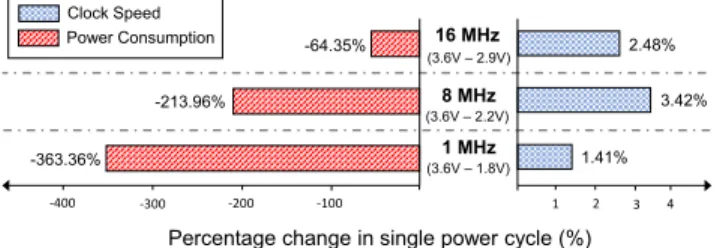
Figure 1. Impact of supply voltage variations on MSP430G2553 clock speed and power consumption in a single power cycle. Existing tools typically ignore these phenomena when modeling the energy consumption of TPC. need to know the worst-case energy costs of given task con-figurations to ensure completion within a single capacitor charge, or forward progress may be compromised.
Observation. Modeling energy consumption of TPCs is an open challenge [17,24,33]. Existing tools are mainly devel-oped for battery-powered embedded devices, which typi-cally enjoy consistent energy supplies for relatively long periods. In contrast, capacitors on TPCs may discharge and recharge several times during a single application run. A single iteration of a CRC code may require up to 17 charges and consequent discharges when harvesting energy from RF transmissions [41]. Single executions of even straight-forward algorithms thus correspond to a multitude of rapid sweeps of an MCU’s operating voltage range [9,41].
We experimentally observe that such a peculiar comput-ing pattern causes severe fluctuations in an MCU’s energy consumption. Fig.1shows example fluctuations we measure on an MSP430G2553 MCU running at 1 MHz in a single power cycle, that is, as it goes from the upper to the lower extreme of the operating voltage range. Power consumption reduces by a factor of up to 363.36%. Clock speed increases by a factor of up to 3.42%. This means the same instruction takes different times depending on the supply voltage at the time it is executed. MSP430-class MCUs are arguably de-facto standard on energy harvesting batteryless platform for both academic [23,42] and commercial ones such as [6], they represent the target platform for many existing TPC system support [16,34,36,41], and currently are the only commercially-available MCUs with non-volatile main mem-ory.
The combined fluctuations of power and clock in Fig.1 cause the energy cost of each MCU cycle to drop by up to 5× in a power cycle. Fig.2shows this behavior as a function of supply voltage, again in a single power cycle. As mentioned earlier, the system may require thousands of power cycles even for a single application iteration; the net effect thus accumulates in the long run.
Unlike dynamic frequency or voltage scaling [39,40] in mainstream computing, these dynamics happen regardless of the system load and the software has no control on them.
Ener gy per MCU cy cle = 1. 59 nJ Ener gy per MC U cy cle = 0 .3 3 nJ Power Consumption Clock Speed
Figure 2. Impact of supply voltage variations on MSP430G2553 power consumption and clock speed. Energy being a product of power (red dotted line) and execution time, which is a function of clock speed (black solid line), the energy cost of a single MCU cycle varies by up to ≈5× depending on the instantaneous supply voltage.
Fluctuations in power consumption are exclusively due to the dynamics in supply voltage and clock speed. In turn, the latter are due to the design of the digitally-controlled oscillators (DCOs) that equip TPCs such as the MSP430-based ones. TI designers confirm that many of their MSP430-class MCUs employ DCOs that cause the clock speed to increase as the supply voltage approaches the lower extreme [29]. This yields better energy efficiency at these regimes, at the cost of varying execution times.
Reasoning on such dynamic behavior is not trivial. For simplicity, a vast fraction of existing literature overlooks these phenomena. Many systems are designed and parame-terized in overly-conservative ways, by considering a con-stant power consumption no matter the supply voltage, and fixed clock speeds [9,17,20,41]. We argue, however, that con-sidering these dynamics is crucial, as their impact magnifies for TPCs with rapid and recurring power cycles.
Contribution. We demonstrate that it is practically possi-ble to accurately model and concretely capitalize on these dynamics. Following background material in Sec.2, our con-tribution is two-pronged:
1. We present in Sec.3a methodology to empirically derive an accurate energy model by measuring the impact of varying voltage supplies on clock speed and power con-sumption for all possible clock configurations. Analytically modeling these dynamics is difficult. For example, power consumption varies according to a nonlinear current draw by the MCU, caused by inductive and capacitative reac-tance of the clock module that uses internal resistors to control the clock speed.
2. The energy model enables the design and implemen-tation of EPIC1, an automated tool that provides accu-rate compile-time energy information, described in Sec.4.
Energy = Power x Time
Voltage Current Clock
Capacitor RSELx DCOx MODx
M S P 4 3 0
Figure 3. Dependencies among quantities determining en-ergy consumption. The direction of the arrows depict the direc-tion of dependency. Power consumpdirec-tion depends upon the input voltage and the current draw. The execution time depends on clock speed. As the supply voltage rapidly varies, additional dependencies are created, shown by black arrows, that perturb an otherwise constant behavior.
EPIC first augments the source code with energy informa-tion at basic-block granularity. It then allows developers to tag a piece of code to determine best- and worst- case energy consumption. We use it to substitute for the con-stant power assumption in existing analysis techniques. To provide evidence of the benefits one can reap by under-standing, modeling, and capitalizing on these dynamics, we report in Sec.5on the use of EPIC in two scenarios. First, we use EPIC with HarvOS [9], a tool to instrument arbitrary code with calls that possibly trigger checkpoints. The accurate energy estimates of EPIC improve HarvOS’ efficiency due to more accurate placement of checkpoint triggers, leading up to a 350% speedup in workload completion times. Next, we plug EPIC within CleanCut [17], a tool supporting task-based programming [17,36]. CleanCut returns warnings whenever it identifies tasks that might accidentally exceed the maxi-mum available energy, impeding forward progress. Using EPIC with CleanCut allows us to ascertain that these warn-ings may be, in fact, bogus. Programmers may thus avoid unnecessary program changes that hurt performance.
We end the paper by discussing the scope of our efforts in Sec.6and concluding remarks in Sec.7.
2
Background and Related Work
We describe the factors that determine the energy consump-tion of TPCs at a fundamental level, to investigate the de-pendencies affected by the dynamics of supply voltage. Next, we discuss how these factors are currently accounted for. Energy estimation. Fig.3graphically depicts the depen-dencies among the relevant quantities. Predicting energy consumption relies on precise values of power consumption and execution time. In embedded MCUs, energy consump-tion is typically estimated by deriving the execuconsump-tion time from the number of clock cycles taken, while power con-sumption is calculated by multiplying the voltage supply with the current draw for a given MCU resistance. Supply voltage depends on the charge of the energy storage facil-ity, which is most often a capacitor in TPCs. Due to their
extensive usage in electronics, accurate capacitor models exist for (dis)charging behavior and voltage drop between the plates [25].
The current drawn by the MCU depends on both the sup-ply voltage and the clock speed. While the former depen-dency is natural (V=IR), the latter stems from internal resis-tance typically controlled through a clock-control register. Sec.3further discusses this aspect for MSP430-class MCUs, which we focus on for the reasons above.
The time factor used to calculate the energy consumption depends, in turn, on the actual clock speed. Embedded MCUs offer specific parameters to configure the clock speed. For ex-ample, MSP430-series MCUs provide three such parameters, called RSELx, DCOx, and MODx, as explained in Sec.3. Existing literature. Existing energy estimation tools [20, 44] model the dependencies shown by grey arrows in Fig.3. For simplicity, however, they tend to overlook the depen-dencies indicated by black arrows and assume constant val-ues for these factors. These tools are often used as input to other systems [9,41] or to guide the programming activ-ities [16,34,36]. The influence of inaccurate models thus percolates up to the run-time performance.
Popular network simulators, such as ns3 and OMNeT++, may employ various energy harvesting models [1,7,43,47]. They are, however, unable to capture the node behavior in a cycle-accurate manner and rather rely on simple approxima-tions, such as coarse-grain estimations of a node’s duty cycle, to enable analysis of energy consumption. These approxima-tions do adopt the assumption of static power supply.
SensEH [18] extends the COOJA/MSPsim framework with models of photovoltaic harvester. The authors explicitly mention the use of static power supply and clock speed models. There exist numerous similar efforts for emulat-ing the behavior of energy harvestemulat-ing in different environ-ments [13,19,37,38]. Allen et al. [2] compare many of these with each other, and discuss their limitations with regard to the representation of energy harvesting dynamics and power consumption modeling. They emphasize the need for more accurate modeling, simulation, and emulation techniques for TPCs, which we provide here.
To improve pre-deployment analysis, existing works ex-plore the use of direct hardware emulation for TPCs. For example, Ekho [22] is a hardware emulator capable of record-ing energy harvestrecord-ing traces in the form of current-voltage surfaces and accurately recreating those conditions in the lab. Custom hardware debuggers [15] for TPCs also exist. Such tools offer the highest accuracy due to their direct in-stallation on the target hardware, but lack the convenience and automation desired at the early stages of development. Ideally, accurate compile-time analysis tools such as EPIC should complement in-field debugging.
No constant power and clock. As discussed in Sec.3, we experimentally observe that the assumption of static supply
voltage is actually not verified in TPCs. As the supply volt-age may potentially traverse the whole operational range multiple times during a single application run, the impact of this unverified assumption is potentially significant. As the supply voltage varies wildly, a ripple effect is created that spreads the variability, over time, to clock speed and, in turn, to current draw. This essentially means that the phenom-ena traverse the dependencies in Fig.3backward, eventually impacting both power consumption and execution time. As a result, these figures are no longer constant, but their val-ues change as frequently as the supply voltage. Both figures ultimately concur to determine energy consumption.
In the next section, we describe the empirical derivation of an energy model that accounts for these phenomena.
3
Energy Modelling Methodology
We describe the methodology to derive models accounting for the dependencies shown by black arrows in Fig.3. First, we discuss modeling the dependency between supply voltage and clock speed. Next, we describe the case of clock speed and current, which ultimately impact power consumption.
To make the discussion concrete, we target MSP430-class MCUs as arguably representative of TPC platforms, although our methodology applies more generally and has a founda-tional nature. Once an energy model is derived for other MCUs, the design of EPIC remains the same. The quantita-tive discussion that follows refer to the energy model we obtain for MSP430G2553 MCU; we find our conclusions to be equally valid for MSP430G2xxx MCUs, based on repeating the same modeling procedures.
3.1 Modeling Clock Drift
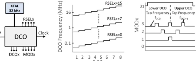
As shown in Fig.4(a), MSP430 MCUs employ a digitally con-trolled oscillator (DCO) that can be configured to deliver clock frequencies from only a few KHz up to 16 MHz.
DCOs on MSP430 MCUs may be configured using three parameters: RSELx, MODx, and DCOx. RSELx stands for resistor-select and is used to configure the DCO for one of the sixteen nominal frequencies in the range 0.06 MHz to 16 MHz. DCOx uses three bits to further subdivide the range selected by RSELx into eight uniform frequency steps as shown in Fig.4(b). Finally, MODx stands for DCO modula-tor and enables the DCO to switch between the configured DCOx and the next higher frequency DCOx+1. The five bits of MODx define 32 different switching-frequencies, as depicted in Fig.4(c), to achieve fine-grained clock control. Measurement procedure. Measuring clock speeds with an oscilloscope is challenging as its probes, when hooked to the clock pin, perturb the DCO impedance. This results in fluctuating measurements.
We thus employ a verified software-based measurement approach used by Texas Instruments for DCO calibra-tion [27]. It consists in counting the number of MCU ticks
DCO RSELx V DCOx MODx Clock XTAL 32 kHz 16 1 0.1 RSELx=15 1 2 3 4 5 6 7 8
DC
O
Fr
equency
(MHz)
DCOx
RSELx=7 RSELx=0 3 2 1 0MODx
Lower DCO Tap Frequency fDCO Upper DCO Tap Frequency fDCO+1 31 (a) MSP430’s DCO module. DCO RSELx V DCOx MODx Clock XTAL 32 kHz 16 1 0.1 RSELx=15 1 2 3 4 5 6 7 8 DC O Fr equency (MHz) DCOx RSELx=7 RSELx=0 3 2 1 0 MODx Lower DCO Tap Frequency fDCO Upper DCO Tap Frequency fDCO+1 31(b) RSELx steps and DCOx range. DCO RSELx V DCOx MODx Clock XTAL 32 kHz 16 1 0.1 RSELx=15 1 2 3 4 5 6 7 8 DC O Fr equency (MHz) DCOx RSELx=7 RSELx=0 3 2 1 0 MODx Lower DCO Tap Frequency fDCO Upper DCO Tap Frequency fDCO+1 31 (c) Modulator pattern.
Figure 4. Impact of DCO parameters on clock.
𝑓𝑒𝑥𝑡 𝑓𝐷𝐶𝑂
A
B
Figure 5. Clock frequency measurements. The number of clock cycles (fDCO) are counted between A and B, namely, two consecutive low to high transitions of the external crystal oscillatorfex t.
within one clock cycle of an external crystal oscillator, as shown in Fig.5. In MSP430 MCUs, the external crystal os-cillator is a very stable clock source offering a frequency of 32.768 KHz. Since the time period of this oscillator is neces-sarily greater than the time period of MCU ticks, we use it to count the number of MCU ticks during its single period. We initialize the Capture/Compare register of Timer_A to Capture mode. The output of DCO is wired to this register and captures Timer_A when a low-to-high transition occurs on the reference signal, that is, the external oscillator. The captured value is the number of clock cycles between two consecutive low-to-high transitions of the reference signal. Empirical model. To model the clock behavior, we sweep the parameter space and empirically record the range of frequencies generated by different DCO configurations.
Altogether, 4096 discrete DCO frequencies can be gener-ated using all possible combinations of RSELx, DCOx, and MODx. As observed in Fig.2, however, the supply voltage impacts the actual clock speed given a certain clock config-uration. For each of these 4096 configurations, we evaluate this impact for the entire operational range of the MCU at 0.001V intervals, and record over 69,888 unique frequencies. These fine-grained measurements allow us to analyze the sensitivity of the clock to supply voltage, and ultimately derive an accurate model.
Analysis. We ask two key questions: i) is the sensitivity of changes in clock speed to variations in supply voltage consistent across all frequencies? and ii) how essential is it to model the clock behavior or, can it be assumed constant?
To answer the first question, in Fig.6(a)we plot the cumu-lative distribution of the percentage difference in clock speed
0 2 4 Difference (%) 0 0.2 0.4 0.6 0.8 1 CDF (a) Frequency. 0 50 100 150 Difference (%) 0 0.2 0.4 0.6 0.8 1 CDF (b) Current. 1x 2x 3x 4x Difference (%) 0 0.2 0.4 0.6 0.8 1 CDF (c) Power.
Figure 6. Impact of voltage supply variations on clock, cur-rent, and power for all DCO configurations. The x-axis shows the difference in the corresponding factor when the voltage drops from one extreme of the MCU’s operational voltage range to the other.
when the voltage drops from one extreme of the MCU’s oper-ational voltage range to the other, across all possible DCO set-tings that determine MCU frequency. The arc-shaped curve in Fig.6(a)implies that the sensitivity of changes in clock speed is not consistent across all frequencies.
We note, however, that this apparent inconsistency is not the outcome of a random clock behavior, but a predictable DCO artifact that is observable in most MSP430 MCUs de-signed for low-power operation. As shown in Fig.7(a), the clock speed changes for a given RSELx when DCOx increases, as well as across increasing RSELx values, for the two ex-tremes of the operational voltage range. TI designers confirm this DCO drift pattern, which is conceded for power conser-vation and is specified as DCO tolerance. The exact circuit design causing this is protected by intellectual property [30]. To answer the second question, we quantify the number of clock cycles that a constant clock model, that is, one that does not incorporate the changes in clock speed as the voltage drops, would not account for. Fig.7(b)shows that this figure increases linearly with every power cycle; more than 10K clock cycles would be unrepresented in only ten power cycles. This could be extremely critical for correctly designing and dimensioning systems that may undergo countless power cycles throughout their lifetime.
3.2 Modeling Dynamic Power Consumption
Changes in supply voltage and clock speed also impact cur-rent draw. A precise curcur-rent model is thus crucial to deter-mine accurate power consumption. While the current drawn by the MCU naturally decreases with voltage and can be cal-culated using Ohm’s law, measuring the impact of a changes in clock speed on current draw is not immediate.
In MSP430 MCUs, the clock speed is mainly controlled by the DCO impedance, which in turn is controlled using the parameters described earlier. This results in varying amounts of current drawn at different frequencies. How-ever, the impedance of the DCO, which can be modeled as an RLC circuit, cannot be derived theoretically since the values of ohmic resistance and reactance are unknown.
0 1 2 3 4 5 6 7 0 1 2 3 4 5 6 7 DCOx 1.45 1.7 1.95 2.2 2.45 2.7 2.95 3.2 Frequency (MHz) 1.54% 2.24% RSEL = 9 RSEL = 8 1.0% 2.82% 1.65% 3.53% 3.6 V 1.8 V
(a) Sensitivity of clock to voltage
0 5 10 # of Power Cycles 0 2000 4000 6000 8000 10000 12000
Unrepresented Clock Cycles
(b)Unrepresented clock cycles @ 8 MHz
Figure 7. Clock behavior. (a) The sensitivity of clock to volt-age increases for a given RSELx when the value of DCOx is increased, as well as across increasing RSELx values. The per-centage values represent the difference in frequency between the two extremes of the operational voltage range; (b) The cup-shaped segments, with each cup corresponding to a single power cycle, show that the number of unrepresented cycle in-creases with the decreasing voltage of the capacitor. Charging times are omitted for brevity.
Measurement procedure. Similar to the clock model, we therefore employ an empirical approach to model the cumu-lative impact of changes in supply voltage and clock speed on current consumption. Our measurement setup includes a 0.1µA resolution multimeter, which measures and automati-cally logs the current drawn by the MCU.
Since the correctness of measurements is critical to derive an accurate model, our approach also caters for the burden voltage—the voltage drop across the measuring instrument— by adding the burden voltageVbto the supplyVs. However, this leads to the current measurements of the MCU at a higher voltageVb+Vs, whereas we need the current draw precisely atVs. As we know the values ofVband the current drawIm, we calculate the resistanceRi of the measuring instrument. We then simply calculate the current draw of the MCU usingImcu = Im−VRbi.
Empirical model. Unlike the sensitivity of clock to varia-tions in supply voltage in Fig.6(a), the current’s sensitivity to variations in clock speed and supply voltage is quite con-sistent and above 100% for a large fraction of frequencies, as shown in Fig.6(b).
The inconsistent behavior for less than 20% observations is mainly due to DCO’s unstable behaviors for very low frequency configurations (below 1 MHz), which are typically neither calibrated nor used with MSP430 MCUs [26]. Fig.6(c) highlights the multiplicative impact of changes in supply voltage and current on an MCU’s power consumption. Power consumption may vary by as much as 3.5× within a single power cycle. This demonstrates that existing tools, as they fail to model such behaviors, tend to provide inaccurate inputs to the design and dimensioning of TPCs.
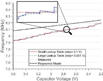
Figure 8. Model representations and their behavior com-pared to empirical measurements @ 8 MHz. Higher precision lookup tables follow closely the actual measurements. The poly-nomial model rests within a 2% error bound.
3.3 Model Representation
We consider two options to represent the results of our mea-surements. Either we use a lookup table or train a model with RSELx, DCOx, MODx and supply voltage (Vs) as inputs. A lookup table is of course, exhaustive, but unlikely to fit on an embedded MCU with tens of KB of main memory, for example, to be used at run-time to implement energy-adaptive behaviors [12,14]. A large lookup table with a pre-cision of three decimal places and a small lookup table with a precision of one decimal place would consume 28 MB and 288 KB in main memory, respectively.
We thus also explore the derivation of a compact model based on linear regression able to fit within a limited memory budget. We ultimately observe that a degree-7 polynomial is sufficient to fit a model with error bound to ±6%. This can be reduced to ±1% with a degree-3 polynomial for common DCO frequencies such as 1 MHz, 8 MHz, and 16 MHz.
Figure8highlights the behavior of these different repre-sentations of the clock model during a single power cycle. A large lookup table with 0.001V precision accurately follows the measurements, whereas a small look up table with 0.1V precision predictably mimics a step function. The polynomial model, in this particular setting, achieves an error below 2%. What model representation to employ is, therefore, to be decided depending on desired accuracy and intended use. Compile-time or off-line analysis may use the lookup table representation, which faithfully describes our measurements. Whenever the models are to be deployed on an embedded MCU with little memory, the polynomial model is easier on memory consumption. Mapper Analyzer Source Code Control Flow Graph Energy Model Assembly Energy Profile get_sign: SUB.W #4, R1 MOV.W #100, 2(R1) MOV.W #1, @R1 CMP.W #100, 2(R1) JNE .L3 MOV.B #1, R12 CMP.W @R1, R12 JL .L3 ADD.W #-5, 2(R1) MOV.W 2(R1), R12 ADD.W R12, R12 1… 2voidget_sign(){ 3 intk = 100; 4 intx = 1; 5 if (k == 100 && x < 2){ 6 k=k-5; 7 k=k*2; 8 k=k+3; 9 } 10 } 11voidmain(){ 12 get_sign(); 13 } "block_id" : “B1", "starting_line" : 3, "ending_line" : 5, "1.9" : [ 5.3, 6.9 ], ... "3.6" : [ 21.6, 28.0 ] } { "block_id" : "B2", "starting_line" : 6, "ending_line" : 8, "1.9" : [ 5.6 ], ... "3.6" : [ 22.9 ] Voltage trace / Capacitor Model Energy Consumption (best/worst case) Ener gy consumption (nJ ) V olt ag e
Figure 9. EPIC code instrumentation process. The mapper maps the assembly instructions to the corresponding basic blocks in the source code and outputs a CFG and energy profile based on the models of Sec.3. The analyzer traverses the CFG to compute best- and worst-case estimates for a given fragment of code and capacitor size.
4
EPIC
Based on the methodology of Sec.3, we develop EPIC: a compile-time analysis tool that accurately predicts energy consumption of arbitrary code segments. Existing solutions employ time-consuming laboratory techniques [9], and yet they overlook the impact of variations in supply voltage. EPIC provides this information in an automated fashion and by explicitly accounting for such dynamics.
4.1 Workflow
EPIC is implemented in two separate Java modules, the map-per and the analyzer, as shown in Fig.9.
Mapper. Inputs for the mapper module are the empirical energy model, a portion of the source code marked by the developer for analysis, and the corresponding assembly code generated for a specific platform. Instructing the compiler to include debugging symbols in the assembly allows the map-per to establish a correspondence between each assembly instruction and the corresponding source code line [32,44] The mapper analyzes the assembly code to find the ba-sic blocks at the level of source code that corresponds to a given set of assembly instructions. Using this mapping and information on the number of MCU cycles for each assembly instructions, EPIC computes the total number of MCU cycles per basic block at the level of source code. This process is non-trivial, as we discuss in Sec.4.2.
Next, the mapper relies on the empirical energy model to predict the energy consumption of each basic block. The output of this step is a separate file, called energy profile, which contains the energy consumption of each basic block at arbitrary supply voltages within the operational range of the target MCU. We store this information in JSON format to facilitate parsing by compile-time tools relying on the output of EPIC. Finally, the mapper also generates the control-flow-graph (CFG) of the code using ANTLR.
Analyzer. The goal of the analyzer is to determine best-and worst-case estimates of energy consumption for each node in the CFG. To that end, the analyzer takes as input the energy profile output by the mapper and a trace of supply voltage values used to determine which value to choose from the energy profile for a particular basic block. Two choices are available for this: either using a capacitor model that simulates the underlying physics and specific (dis)charging behaviors, or relying on a user-provided energy trace that indicates the state of capacitor’s charge over time.
Similar to other compile-time tools, best- and worst-case estimates are the best output EPIC can provide. There are cases where these estimates depend on run-time informa-tion; for example, in the presence of loops whose number of iterations is not known at compile time. If a user-specified piece of code also includes any of these constructs, EPIC prompts the user for providing an estimate of the missing information to be considered in a given analysis.
4.2 Finding MCU Cycles per Basic Block
Established techniques exist to map basic blocks at the level of source code to assembly instructions, for example, as in PowerTOSSIM [44] and TimeTOSSIM [32]. These techniques, however, do not accurately handle cases where a basic block of source code may correspond to the execution of a vari-able number of instructions in assembly; therefore, a single node in the CFG is translated into multiple basic blocks at the assembly level. Short-circuit evaluation, for loops, and compiler-inserted libraries are examples where issues mani-fest that may cause a loss of accuracy in energy estimates.
To handle these cases, EPIC further dissects the mapping process to extract additional information useful to reason on the energy consumption of a given basic block.
Short-circuit evaluations. These include concatenations of logical operators, such as “&&” or “||”, where the truth value of a pre-fix determines the truth value of the whole expression. The assembly code generated by the compiler skips the evaluation of the post-fix part of the expression as soon as the pre-fix determines the whole expression.
To handle these cases, the mapper reports the energy con-sumption of all possible evaluations of the statement in-volving these operators. This is shown in the energy profile of Fig.9for the if statement at line 5. Two separate values
are reported for its basic block (B1): one for only the pre-fix and one for the complete evaluation of the expression.
This information is then useful for the analyzer module, which may choose the appropriate value depending upon the type of analysis required. For example, when considering the best-case energy consumption, the analyzer considers the energy consumption for executing the minimal pre-fix that determines the truth value. Differently, the analyzer accounts for the energy consumption of executing every sub-expression when computing the worst case.
Loops using for. Execution of for loops may cost a dif-ferent number of cycles at the first or at intermediate itera-tion(s). This is because the initialization of the loop variable is only performed at the first iteration, whereas all other iter-ations incur the same number of MCU cycles as they always perform the same operations; for example, incrementing a counter and checking its value against a threshold.
The mapper accurately identifies the set of instructions needed for these two different types of execution of the for(;;)statements, and reports them in the energy profile as two separate entries for the corresponding basic block. The analyzer then utilizes this information to accurately calculate the energy consumption of different loop iterations. Compiler-inserted functions. For programming con-structs that are not supported natively in hardware, compil-ers insert their own library functions to emulate the func-tionality in software. For example, if an MCU has no floating point support, the compiler automatically replaces the corre-sponding statements with its own assembly code. Since there are only a handful of such library functions typically, we profiling these with arbitrary inputs as function arguments and record their best- and worst-case energy consumption.
5
Evaluation
We start by evaluating the accuracy of energy profile infor-mation returned by EPIC across four benchmark applications, before employing the entire EPIC workflow for compile-time analysis in two concrete cases.
5.1 Microbenchmarks
Measuring the accuracy of EPIC output is a stepping stone to investigate the use of EPIC in a concrete case study. The accu-racy of energy profile information returned by EPIC depends on i) the accuracy of the empirical energy model described in Sec.3, and ii) the effectiveness of the mapping techniques between source code and assembly code of Sec.4.2.
Our benchmarks include open-source implementations of Bubblesort, CRC, FFT, and AES, which are often employed for benchmarking system support for TPCs [5,31,41]. We run each application on real hardware at different supply voltages and record a per-basic-block trace of execution time and current draw to compute the energy consumption.
Table 1. EPIC accuracy.
Voltage Measured Energy Predicted Energy Error Applications (V) (µJ) (µJ) (%) 2.3 0.9016 0.9014 -0.03 2.5 1.0332 1.0354 0.21 3.0 1.5538 1.5556 0.12 Bubble Sort 3.5 2.1960 2.1956 -0.02 2.3 0.3709 0.3697 -0.31 2.5 0.4267 0.4248 -0.45 3.0 0.6389 0.6382 -0.12 CRC 3.5 0.9027 0.9007 -0.22 2.3 12.9904 13.0194 0.22 2.5 14.9520 14.9554 0.02 3.0 22.4640 22.4695 0.02 FFT 3.5 31.5952 31.7129 0.37 2.3 37.3888 37.5609 0.46 2.5 42.9240 43.1463 0.52 3.0 64.3968 64.8247 0.66 AES 3.5 90.9664 91.4920 0.58
Table1compares the results returned by EPIC at differ-ent supply voltages with the measures on an MSP430G2553 running at 8 MHz. The error is generally well below 1%. The results demonstrate that the information input to the ana-lyzer module is accurate, as a result of the accuracy of the empirical model and the specific mapping between source code and assembly we adopt.
5.2 EPIC with HarvOS
We integrate EPIC with HarvOS [9], an existing system sup-port for TPCs. HarvOS relies on compile-time energy es-timates to insert checkpoint triggers that possibly take a checkpoint whenever a device is about to exhaust the energy. The triggers include code to query the current state of the energy buffer for deciding whether or not to checkpoint. Checkpoints are costly in energy and additional execution time. Regardless of whether a checkpoint takes place, these calls represent an overhead anyways, as merely querying the energy buffer does consume energy [41].
In HarvOS [9], the placement of trigger calls is based on an efficient strategy that requires a worst-case estimate of the energy consumption of each node in the CFG. Similar to existing literature, HarvOS normally employs a manual in-strumentation process based on a static energy consumption model, namely, overlooking the dynamic behavior of power consumption and clock speeds. We use EPIC to substitute for such manual instrumentation process.
Setup. We use two applications: i) an Activity Recognition (AR) application that recognizes human activity based on sensor values, often utilized for evaluating TPC solutions [16, 34], and ii) an implementation of the Advanced Encryption Standard (AES), which is one of the benchmarks used in HarvOS [9]. We execute EPIC by relying on two different types of voltage traces as an input to the analyzer module.
First, we use a fundamental voltage trace often found in existing literature [8,31,41,49]. The device boots with the capacitor fully charged, and computes until the capacitor is
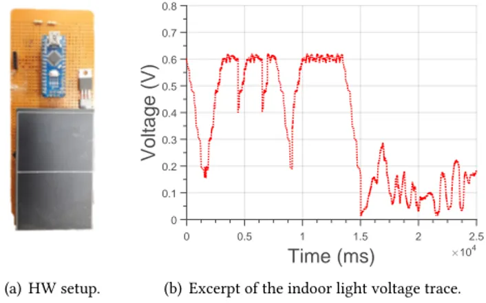
(a) HW setup. Time (ms) #104 0 0.5 1 1.5 2 2.5 Voltage (V) 0 0.1 0.2 0.3 0.4 0.5 0.6 0.7 0.8
(b) Excerpt of the indoor light voltage trace.
Figure 10. Voltage trace from indoor light using a mono-crystalline solar panel.
empty again. In the meantime, the environment provides no additional energy. Once the capacitor is empty, the environ-ment provides new energy until the capacitor is full again and computation resumes. This specific energy provisioning pattern generates executions that are highly intermittent, namely, executions that most paradigmatically differentiate TPCs from other platforms. This profile is also representative of TPC applications based on wireless energy transfer [10]. With this technology, devices are quickly charged with a burst of wirelessly-transmitted energy until they boot. Next, the application runs until the capacitor is empty again. The device rests dormant until another burst of wireless energy comes in. We call this trace the decay trace.
Second, we use a voltage trace collected using a mono-crystalline high-efficiency solar panel [46], placed on a desk and harvesting energy from light in an indoor lab environ-ment, as shown in Fig.10. We use an Arduino Nano [4] to log the voltage output across the load, equivalent to the re-sistance of an MSP430G2553 in active mode, attached to the solar panel. We call this trace the light trace.
Results. We compare features and performance of HarvOS-instrumented code using manual energy profiling as in the original HarvOS, against using HarvOS with the energy esti-mates of EPIC as input, based on an MSP430G2553 running at 8MHz. We note that:
1. Using EPIC, the number of trigger calls inserted by HarvOS in the original code reduces;
2. A more accurate code instrumentation due to EPIC leads to fewer checkpointing interruptions at run-time. The first two columns in Table2show the results of the instrumentation process when using the smallest capacitor size needed to complete the given workloads. We consider this as TPCs typically prefer smaller capacitors as energy buffer, because they reach the operating voltage more quickly and yield smaller device footprints. However, if the capacitor
Table 2. Features and performance of HarvOS-instrumented code with and without EPIC.
# of trigger calls # of checkpoints Speedup in
App Manual EPIC Manual EPIC time (%)
Decay Trace AR 2 1 85 42 51.66 AES 3 0 2 0 354.97 Light Trace AR 2 1 64 32 49.35 AES 3 0 1 0 203.31
is too small, a system may be unable to complete checkpoints, impeding any progress.
For the AR application, EPIC’s accurate energy estimates halve the number of trigger calls that HarvOS places in the code. This reduction occurs due to EPIC’s ability to accu-rately model the varying number of clock cycles at differ-ent voltages that a static model would not consider. As the voltage of the capacitor decreases, the speed of the clock in-creases. This results in more clock cycles becoming available per unit of time at lower supply voltages. Not accounting for such dynamic behavior significantly underestimates the number of clock cycles available within a single time unit in conditions of low supply voltages.
The results for AES instrumentation are revealing: based on the energy estimates provided by EPIC, HarvOS decides to place no trigger calls. EPIC thus indicates that the energy provided by the capacitor is sufficient for the AES imple-mentation to complete in a single power cycle, and thus no checkpoints are ever necessary. This contrasts the outcome of the HarvOS compile-time analysis based on the assump-tion of constant power consumpassump-tion and clock speed. In that case, HarvOS would still place three trigger calls within the code, uselessly incurring the corresponding overhead. This shows how not accounting for the dynamic behaviors we study here profoundly misguides compile-time analysis.
The impact of the trigger call placement with or without EPIC has marked consequences when running the instru-mented applications. The third and fourth columns in Table2 show the corresponding results for either voltage trace. The AR application instrumented by HarvOS based on the energy estimates of EPIC completes the execution with nearly 50% fewer checkpoints. Similarly, the successful completion of the AES implementation without a single checkpoint con-firms the validity of the energy estimates of EPIC, which prompts HarvOS not to place any trigger call.
Checkpoint operations are extremely energy consuming, as they incur operations on non-volatile memory. Fewer checkpoints allow the system to spend the corresponding energy budget in thousands of useful computation cycles, which are otherwise wasted due to inaccurate insertion of trigger calls in the original HarvOS. Thus, the system pro-gresses faster towards the completion of the workload. The
Capacitor (uF) 15 20 25 30 35 40 45 50 # of checkpoints 0 20 40 60 80 100 120 Manual EPIC
(a) AR with decay trace.
Capacitor (uF) 10 20 30 40 50 # of checkpoints 0 20 40 60 80 100 120 Manual EPIC
(b) AR with light trace.
Capacitor (uF) 5 10 15 20 25 30 35 # of checkpoints 0 1 2 3 4 5 Manual EPIC
(c) AES with decay trace.
Capacitor (uF) 5 10 15 20 25 30 35 # of checkpoints 0 1 2 3 4 5 Manual EPIC
(d) AES with light trace.
Figure 11. HarvOS results. The benefits of using EPIC within HarvOS apply across different capacitor sizes.
right most column in Table2quantifies the benefits in terms of speedup of completion time for the given workload.
Fig.11further investigates the execution of either applica-tion at increasing capacitor sizes. These results affirm that the benefits of using EPIC within HarvOS are not just limited to the smallest capacitor that ensures completion. The appar-ent outlier at 40uF in Fig.11(b)is due to a specific behavior of HarvOS whenever larger capacitors simultaneously yield a change in the placement of trigger calls and in their over-all number [9]. For the AR application, the corresponding speedup in completion time range from 14% at 35uF with the decay trace, to 159% at 40uF using the light trace. For the AES implementation, Table2already shows the performance range, as no checkpoints are needed.
Finally, Fig.11also shows that in a number of situations, the compile-time instrumentation generated by HarvOS when using the energy estimates of EPIC yields an oper-ational system at much smaller capacitor sizes, as com-pared with the original HarvOS. The cost for the overly-conservative estimations in the latter, based on static power consumption and clock speeds, materialize in the inability to complete when using small capacitors. In contrast, EPIC captures the dynamic behavior of these figures and offers ac-curate estimations to HarvOS; this results in more informed decisions on trigger call placement and smarter decisions on whether to checkpoint when executing a trigger call.
5.3 EPIC with CleanCut
An alternative to using automated placement of trigger calls is to employ task-based programming abstractions offering transactional semantics [16, 34, 36]. Programmers are to manually define tasks that are guaranteed to either complete by committing their output to non-volatile memory, or to have no effect on program state.
CleanCut [17] is a compile-time tool that helps program-mers using these abstractions identify non-termination bugs. These bugs exist whenever a task definition includes execu-tion paths whose energy cost exceeds the maximum available energy, based on capacitor size. If no new energy is harvested while executing, a task may never complete and thus the program ends up in a livelock situation, always resuming from the beginning of the last successfully executed task.
CleanCut relies on an energy model obtained through hardware-assisted profiling. The model estimates the energy consumption of each basic block at near maximum voltage supply, to avoid underestimations. The estimates are then convoluted across the possible execution paths in a task to find energy distributions for individual tasks. Based on this, CleanCut returns warnings whenever it suspects a non-termination bug. Programmers must then defend against these; for example, by refactoring the code to define shorter tasks. This is not just laborious, but also detrimental to per-formance, as every task boundary incurs significant energy overhead due to committing results on non-volatile memory. Colin et al. [17] argue that an accurate model may pro-vide more genuine warnings, but was out of scope. Using EPIC with CleanCut, we prove this argument. For long exe-cution paths in a task that use the capacitor to near depletion, the difference between the actual used energy—accurately modeled by EPIC—and CleanCut’s estimations obtained as described above, can be significant. This results in false posi-tives, that is, non-termination bugs are suspected for paths that may safely complete with the given energy budget. Setup. We use the same applications as in CleanCut [17]: i) an Activity Recognition (AR) application similar to Sec.5.2, ii) a Cuckoo Filter (CF) that efficiently tests set membership, iii) a Coldchain Equipment Monitor (CEM) application, and iv) an implementation of the RSA algorithm.
The placement of task boundaries in all applications is the one of CleanCut [17]. We then estimate the energy consump-tion of every possible execuconsump-tion path in a task using CleanCut with EPIC, compared with CleanCut using a synthetic model that safely approximates that of CleanCut, whose hardware and source code are not available. This model follows the recommendation that the energy consumption of each ba-sic block should be estimated near the maximum voltage to avoid underestimations [17].
We use a 10µF capacitor as found on Intel WISP 4.1 devices, and consider an MSP430G2553 running at 8 MHz.
Table 3. CleanCut non-termination bug warnings with and without EPIC. Application Task boundaries Paths CleanCut warnings EPIC warnings AR 4 147 8 0 RSA 4 8 3 0 CF 11 25 0 0 CEM 11 20 0 0 5 10 15 20 Path 0 10 20 30 40 50 60 Energy (uJ) 2 2.5 3 3.5 Capacitor Voltage (V) CleanCut CleanCut + EPIC Device Capacity
(a) Activity Recognition (AR).
1 2 3 4 5 6 7 8 Path 0 10 20 30 40 50 60 Energy (uJ) 2 2.5 3 3.5 Capacitor Voltage (V) CleanCut CleanCut + EPIC Device Capacity (b) RSA. 0 5 10 15 20 25 Path 0 10 20 30 40 50 60 Energy (uJ) 2 2.5 3 3.5 Capacitor Voltage (V) CleanCut CleanCut + EPIC Device Capacity (c) Cuckoo Filter (CF). 5 10 15 20 Path 0 10 20 30 40 50 60 Energy (uJ) 2 2.5 3 3.5 Capacitor Voltage (V) CleanCut CleanCut + EPIC Device Capacity (d) CEM.
Figure 12. CleanCut results. Using EPIC with CleanCut, false positives are avoided when looking for non-termination bugs.
Results. Table3summarizes our results, which are further detailed in Fig.12. By comparing how the two solutions build up the energy estimates for a task, we note that the two start identical, but as paths become longer and nears the capacitor’s limit, CleanCut starts to overestimate. This is because it uses the same energy model for every basic block, regardless of where it appears on the path.
The results for the AR application, shown in Fig.12(a), indicate that CleanCut returns eight false positives, in that it estimates the energy consumption of those paths to exceed the available capacitor energy. Developers would then need to break those tasks in smaller units, investing additional effort and causing increased overhead at run-time due to more frequent commits to non-volatile memory at the end of shorter tasks. This is not the case with CleanCut using EPIC, which verifies that the same execution paths may complete successfully. Task definitions thus include no non-termination bugs; therefore, developers need not to spend any additional effort and the system runs with better energy efficiency. Similar considerations apply to RSA algorithm, wherein the original design of CleanCut returns three false positives, as shown in Fig.12(b).
In the case of CF, processing is generally lighter com-pared to AR and RSA. Further, the existing task definition includes very short tasks already. As a result, the estimates of CleanCut and CleanCut using EPIC are close to each other, as shown in Fig.12(c)No warnings for possible non-termination bugs are returned. Similar considerations apply also to the CEM application, whose results are shown in Fig.12(d).
CleanCut also provides a task boundary placer that auto-matically breaks long tasks. We cannot evaluate the impact of EPIC there, since the implementation is not available, but we argue that the benefits would be even higher. In fact, CleanCut’s placer is actively trying to bring task definitions to their optimal energy point, that is, closer to the capacitor limit. This is precisely where the difference in estimates be-tween the CleanCut and CleanCut with EPIC is maximum. Thus, the probability of paths landing in the region where the original design of CleanCut declares a task to be too long, but CleanCut using EPIC says the opposite, is likely higher compared to checking a manual placement.
6
Discussion
We provide next due considerations on how our work is cast in the larger TPC domain.
MCUs and peripherals. We focus on the MCU as it co-ordinates the functioning of the entire system when using the emerging federated energy architectures [23]. For the MCU, accurately forecasting the energy cost of a certain frag-ment of code is key to dimensioning capacitors and setting its running frequency. Peripheral operation may be post-poned when the energy is insufficient or the system may impose atomic executions on peripheral operations [16,36]. Dedicated works exist that ensures the correct intermittent operation of peripherals [35,45,50].
We also model the active mode of the MCU as this is the only mode where the MCU executes the code [48]. TPCs pri-marily use this mode to maximize throughput during power cycles that may be as short as a few ms. Other low-power modes are typically used in battery-powered platforms for conserving energy when idle.
Voltage regulation. Voltage regulators are commonly found in computer power supplies to stabilize the supply voltage. Despite the availability of efficient voltage regulators with minimal dropout [28], they are typically not employed in TPCs [23] because step-up regulators reduce the power cycle duration and step-down regulators can critically fail some on-chip components. When deploying Mementos [41] on the voltage-regulated WISP platform, the authors report a one-half reduction in the duration of power cycles when using a 2.8V step-up regulator, and checkpointing failures with a 1.8V step-down regulator due to failing to meet the voltage requirements of flash memory. An open research question is what are the conditions, for example, in terms of
energy provisioning patterns, where the trade-off exposed by dynamic regulation of voltage play favorably.
7
Conclusion
We demonstrated that it is practically possible to capital-ize on the dynamic energy consumption patterns of TPCs. We presented a methodology to experimentally build an ac-curate energy model, accounting for variations in power consumption and clock speed. We use EPIC, a compile-time tool, as an instrument to quantify the impact of these models. When integrated with HarvOS, EPIC enables 350% speedup in workload completion times, and similarly avoids unneces-sary program changes that ultimately hurt energy efficiency when used with CleanCut. Based on the evidence we col-lect with EPIC, we conclude that it is possible to account for the dynamic behaviors of energy consumption without sacrificing simplicity of analysis.
References
[1] Muhammad Hamad Alizai, Qasim Raza, Yasra Chandio, Affan A. Syed, and Tariq M. Jadoon. 2016. Simulating Intermittently Powered Em-bedded Networks. In Proceedings of the 2016 International Conference on Embedded Wireless Systems and Networks (EWSN ’16). Junction Publishing, USA, 35–40.
[2] James Allen, Matthew Forshaw, and Nigel Thomas. 2017. Towards an Extensible and Scalable Energy Harvesting Wireless Sensor Network Simulation Framework. In Proceedings of the 8th ACM/SPEC on Inter-national Conference on Performance Engineering Companion (ICPE ’17 Companion). ACM, New York, NY, USA, 39–42.
[3] Patricia Anacleto, PM Mendes, E Gultepe, and DH Gracias. 2012. 3D small antenna for energy harvesting applications on implantable micro-devices. In Antennas and Propagation Conference (LAPC). IEEE, 1–4. [4] ARDUINO. 2018. NANO. https://store.arduino.cc/usa/arduino-nano
((accessed 2018-10-28)).
[5] Domenico Balsamo, Alex S Weddell, Geoff V Merrett, Bashir M Al-Hashimi, Davide Brunelli, and Luca Benini. 2015. Hibernus: Sustaining Computation During Intermittent Supply for Energy-Harvesting Sys-tems. Embedded Systems Letters 7, 1 (2015).
[6] Medusa-M2233 UHF RFID battery-free device. [n. d.]. Farsens. http: //www.farsens.com/en/products/medusa-m2233/((accessed 2019-03-04)).
[7] David Benedetti, Chiara Petrioli, and Dora Spenza. 2013. GreenCastalia: An Energy-harvesting-enabled Framework for the Castalia Simulator. In Proceedings of the 1st International Workshop on Energy Neutral Sensing Systems (ENSSys ’13). ACM, New York, NY, USA, Article 7, 6 pages.
[8] Naveed Bhatti and Luca Mottola. 2016. Efficient state retention for transiently-powered embedded sensing. In International Conference on Embedded Wireless Systems and Networks. 137–148.
[9] Naveed Anwar Bhatti and Luca Mottola. 2017. HarvOS: Efficient code instrumentation for transiently-powered embedded sensing. In Information Processing in Sensor Networks (IPSN), 2017 16th ACM/IEEE International Conference on. IEEE, 209–220.
[10] Naveed Anwar Bhatti, Affan Ahmed Syed, and Muhammad Hamad Alizai. 2014. Sensors with Lasers: Building a WSN Power Grid. In Proc. 13t hInt. Symp. Information Processing in Sensor Networks (IPSN ’14).
261–272.
[11] Naveed Anwar Bhatti, Affan Ahmed Syed, Muhammad Hamad Alizai, and Luca Mottola. 2016. Energy Harvesting and Wireless Transfer in Sensor Network Applications: Concepts and Experiences. ACM
Transactions on Sensor Networks (TOSN) (2016).
[12] Michael Buettner, Benjamin Greenstein, and David Wetherall. 2011. Dewdrop: An Energy-Aware Runtime for Computational RFID. In Proceedings of the 8th USENIX Symposium on Networked Systems Design and Implementation, NSDI 2011, Boston, MA, USA, March 30 - April 1, 2011.
[13] Andrea Castagnetti, Alain Pegatoquet, Cécile Belleudy, and Michel Auguin. 2012. A framework for modeling and simulating energy harvesting WSN nodes with efficient power management policies. EURASIP J. Emb. Sys. 2012 (2012), 8.
[14] Geoffrey Werner Challen, Jason Waterman, and Matt Welsh. 2010. IDEA: Integrated Distributed Energy Awareness for Wireless Sensor Networks. In Proceedings of the 8th International Conference on Mobile Systems, Applications, and Services (MobiSys ’10). ACM, New York, NY, USA, 35–48.
[15] Alexei Colin, Graham Harvey, Brandon Lucia, and Alanson P. Sample. 2016. An Energy-interference-free Hardware-Software Debugger for Intermittent Energy-harvesting Systems. SIGOPS Oper. Syst. Rev. 50, 2 (March 2016), 577–589.
[16] Alexei Colin and Brandon Lucia. 2016. Chain: Tasks and Channels for Reliable Intermittent Programs. In Proceedings of the 2016 ACM SIGPLAN International Conference on Object-Oriented Programming, Systems, Languages, and Applications (OOPSLA 2016). ACM, New York, NY, USA, 514–530. https://doi.org/10.1145/2983990.2983995
[17] Alexei Colin and Brandon Lucia. 2018. Termination checking and task decomposition for task-based intermittent programs. In Proceedings of the 27th International Conference on Compiler Construction. ACM, 116–127.
[18] Riccardo Dall’Ora, Usman Raza, Davide Brunelli, and Gian Pietro Picco. 2014. SensEH: From simulation to deployment of energy harvesting wireless sensor networks. In IEEE 39th Conference on Local Computer Networks, Edmonton, AB, Canada, 8-11 September, 2014 - Workshop Proceedings. 566–573.
[19] Amine Didioui, Carolynn Bernier, Dominique Morche, and Olivier Sentieys. 2013. HarvWSNet: A co-simulation framework for energy harvesting wireless sensor networks. In International Conference on Computing, Networking and Communications, ICNC 2013, San Diego, CA, USA, January 28-31, 2013. 808–812.
[20] Joakim Eriksson, Adam Dunkels, Niclas Finne, Fredrik Osterlind, and Thiemo Voigt. 2007. Mspsim–an extensible simulator for msp430-equipped sensor boards. In Proceedings of the European Conference on Wireless Sensor Networks (EWSN), Poster/Demo session, Vol. 118. [21] Joaquín Gutiérrez, Juan Francisco Villa-Medina, Alejandra
Nieto-Garibay, and Miguel Ángel Porta-Gándara. 2014. Automated irrigation system using a wireless sensor network and GPRS module. IEEE trans-actions on instrumentation and measurement 63, 1 (2014), 166–176. [22] Josiah Hester, Timothy Scott, and Jacob Sorber. 2014. Ekho: Realistic
and Repeatable Experimentation for Tiny Energy-harvesting Sensors. In Proceedings of the 12th ACM Conference on Embedded Network Sensor Systems (SenSys ’14). ACM, New York, NY, USA, 1–15.
[23] Josiah Hester and Jacob Sorber. 2017. Flicker: Rapid Prototyping for the Batteryless Internet-of-Things. In Proceedings of the 15th ACM Conference on Embedded Network Sensor Systems (SenSys). ACM, 19. [24] Josiah Hester and Jacob Sorber. 2017. The Future of Sensing is
Bat-teryless, Intermittent, and Awesome. In Proceedings of the 15th ACM Conference on Embedded Network Sensor Systems (SenSys ’17). ACM, New York, NY, USA, Article 21, 6 pages.
[25] Paul Horowitz and Winfield Hill. 1989. The art of electronics. Cambridge Univ. Press.
[26] Texas Instruments. 2018. Getting Started with the MSP430 LaunchPad.
https://goo.gl/6ueTEC((accessed 2018-10-28)).
[27] Texas Instruments. 2018. Manual. http://www.ti.com/lit/an/slaa336a/ slaa336a.pdf(accessed 2018-03-08).
[28] Texas Instruments. 2018. Power-management integrated chip (PMIC).
https://goo.gl/45psWK((accessed 2018-10-28)).
[29] Texas Instruments. 2018. TI E2E Coummunity.https://goo.gl/XxrhN3
((accessed 2018-10-28)).
[30] Texas Instruments. 2018. TI E2E Coummunity.https://goo.gl/dPbNkJ
((accessed 2018-10-28)).
[31] Hrishikesh Jayakumar, Arnab Raha, Woo Suk Lee, and Vijay Raghu-nathan. 2015. QuickRecall: A HW/SW Approach for Computing Across Power Cycles in Transiently Powered Computers. J. Emerg. Technol. Comput. Syst. 12, 1 (2015).
[32] Olaf Landsiedel, Muhammad Hamad Alizai, and Klaus Wehrle. 2008. When Timing Matters: Enabling Time Accurate and Scalable Simu-lation of Sensor Network Applications. In Proceedings of the 7th In-ternational Conference on Information Processing in Sensor Networks, IPSN 2008, St. Louis, Missouri, USA, April 22-24, 2008. 344–355. https: //doi.org/10.1109/IPSN.2008.31
[33] Brandon Lucia, Vignesh Balaji, Alexei Colin, Kiwan Maeng, and Emily Ruppel. 2017. Intermittent Computing: Challenges and Opportuni-ties. In 2nd Summit on Advances in Programming Languages (SNAPL 2017). Schloss Dagstuhl–Leibniz-Zentrum fuer Informatik, Dagstuhl, Germany, 8:1–8:14.
[34] Brandon Lucia and Benjamin Ransford. 2015. A Simpler, Safer Program-ming and Execution Model for Intermittent Systems. In Proceedings of the 36th ACM SIGPLAN Conference on Programming Language De-sign and Implementation (PLDI) (PLDI ’15). ACM, New York, NY, USA, 575–585. https://doi.org/10.1145/2737924.2737978
[35] Giedrius Lukosevicius, Alberto Rodriguez Arreola, and Alex S Wed-dell. 2017. Using sleep states to maximize the active time of transient computing systems. In Proceedings of the Fifth ACM International Work-shop on Energy Harvesting and Energy-Neutral Sensing Systems (EnSys). ACM, 31–36.
[36] Kiwan Maeng, Alexei Colin, and Brandon Lucia. 2017. Alpaca: Inter-mittent Execution Without Checkpoints. Proc. ACM Program. Lang. 1, Object-Oriented Programming Systems, Languages, and Applications (OOPSLA), Article 96 (Oct. 2017), 30 pages.
[37] Geoff V. Merrett, Neil M. White, Nick R. Harris, and Bashir M. Al-Hashimi. 2009. Energy-Aware Simulation for Wireless Sensor Net-works. In Proceedings of the Sixth Annual IEEE Communications Society Conference on Sensor, Mesh and Ad Hoc Communications and Networks, SECON 2009, June 22-26, 2009, Rome, Italy. 1–8.
[38] Pieter De Mil, Bart Jooris, Lieven Tytgat, Ruben Catteeuw, Ingrid Moerman, Piet Demeester, and Ad Kamerman. 2010. Design and Implementation of a Generic Energy-Harvesting Framework Applied to the Evaluation of a Large-Scale Electronic Shelf-Labeling Wireless Sensor Network. EURASIP J. Wireless Comm. and Networking 2010 (2010).
[39] Kevin J Nowka, Gary D Carpenter, Eric W MacDonald, Hung C Ngo, Bishop C Brock, Koji I Ishii, Tuyet Y Nguyen, and Jeffrey L Burns. 2002. A 32-bit PowerPC system-on-a-chip with support for dynamic voltage scaling and dynamic frequency scaling. IEEE Journal of Solid-State Circuits 37, 11 (2002), 1441–1447.
[40] Padmanabhan Pillai and Kang G Shin. 2001. Real-time dynamic voltage scaling for low-power embedded operating systems. In ACM SIGOPS Operating Systems Review, Vol. 35. ACM, 89–102.
[41] Benjamin Ransford, Jacob Sorber, and Kevin Fu. 2011. Mementos: Sys-tem Support for Long-running Computation on RFID-scale Devices. In Proc. 16t hInt. Conf. Architectural Support for Programming Languages and Operating Systems (ASPLOS XVI). 159–170.
[42] Alanson P Sample, Daniel J Yeager, Pauline S Powledge, Alexander V Mamishev, Joshua R Smith, et al. 2008. Design of an RFID-Based Battery-Free Programmable Sensing Platform. IEEE Transactions on Instrumentation and Measurement 57, 11 (2008).
[43] Antonio Sánchez, Salvador Climent, Sara Blanc, Juan Vicente Capella, and Ignacio Piqueras. 2011. WSN with Energy-harvesting: Modeling and Simulation Based on a Practical Architecture Using Real Radiation
Levels. In Proceedings of the 6th ACM Workshop on Performance Moni-toring and Measurement of Heterogeneous Wireless and Wired Networks (PM2HW2N ’11). ACM, New York, NY, USA, 17–24.
[44] Victor Shnayder, Mark Hempstead, Bor-Rong Chen, and Matt Welsh. 2004. PowerTOSSIM: Efficient Power Simulation for TinyOS Appli-cations. In Proceedings of the ACM Conference on Embedded Network Sensor Systems (SenSys).
[45] Rebecca Smith and Scott Rixner. 2015. Surviving Peripheral Failures in Embedded Systems.. In USENIX Annual Technical Conference. 125–137. [46] IXYS SolarMD. 2018. SLMD481H08L.http://ixapps.ixys.com/((accessed
2018-10-28)).
[47] Cristiano Tapparello, Hoda Ayatollahi, and Wendi Heinzelman. 2014. Energy Harvesting Framework for Network Simulator 3 (Ns-3). In Pro-ceedings of the 2Nd International Workshop on Energy Neutral Sensing
Systems (ENSsys ’14). ACM, New York, NY, USA, 37–42.
[48] TI. 2018. Data Sheet. http://www.ti.com/lit/ds/symlink/msp430g2353. pdf(accessed 2018-02-18).
[49] Joel Van Der Woude and Matthew Hicks. 2016. Intermittent Compu-tation Without Hardware Support or Programmer Intervention. In Proceedings of the 12th USENIX Conference on Operating Systems De-sign and Implementation (OSDI’16). USENIX Association, Berkeley, CA, USA, 17–32. http://dl.acm.org/citation.cfm?id=3026877.3026880
[50] Kasim Sinan Yildirim, Amjad Yousef Majid, Dimitris Patoukas, Koen Schaper, Przemyslaw Pawelczak, and Josiah Hester. 2018. InK: Reac-tive Kernel for Tiny Batteryless Sensors. In Proceedings of the ACM Conference on Embedded Network Sensor Systems (SenSys).