Spectrum sensing through implementation of USRP2

(1)

Master Thesis

Electrical Engineering Thesis no: MEE-27675 November 2010

Spectrum Sensing Through

Implementation of USRP2

Adnan Aftab

(2)

This thesis is submitted to the School of Computing at Blekinge Institute of Technology in partial fulfillment of the requirements for the degree of Master of Science in Electrical Engineering. The thesis is equivalent to 20 weeks of full time studies.

Contact Information: Authors:

Adnan Aftab

E-mail: adnan.aftab@ymail.com Muhammad Nabeel Mufti

E-mail: nabeel.mufti@gmail.com

University advisor: Alexandru Popescu School of Computing

School of Computing

Blekinge Institute of Technology 371 79 Karlskrona

Internet : www.bth.se/com Phone : +46 455 38 50 00 Fax : +46 455 38 50 57

(3)

A

CKNOWLEDGMENT

We really want to thank our supervisor Mr. Alexandru Popescu for his time, guidance, support and friendly attitude towards us all the time. His valuable advices paved the way for our research. We would like to extend our thanks to Dr. David Erman for providing us the experimental equipments and to Mr. Yong Yao, his interest towards our research and guiding us from precision towards accuracy. We would also like to thank our families for their support, both financially and morally. Last but not least we like to say thanks to our friends in Sweden, they make our stay memorable and joyful.

(4)

A

BSTRACT

Scarcity of the wireless spectrum has led to the development of new techniques for better utilization of the wireless spectrum. Demand for high data rates and better voice quality is resulting in the development of new wireless standard making wireless spectrum limited than ever. In this era of wireless communication, service providers and telecom operators are faced with a dilemma where they need a large sum of the wireless spectrum to meet the ever increasing quality of service requirements of consumers. This has led to the development of spectrum sensing techniques to find the unused spectrum in the available frequency band.

The results presented in this thesis will help out in developing clear understanding of spectrum sensing techniques. Comparison of different spectrum sensing approaches. The experiments carried out using USRP2 and GNU radio will help the reader to understand the concept of underutilized frequency band and its importance in Cognitive Radios.

(5)

List of abbreviations

Acronym Description

A Ampere

ADC Analogue to Digital Converter CPC Cognition enabling pilot channel

CPU Central processing unit

DAC Digital to analogue converter

dBm Milliwatt-decibel

DC Direct current

DDC Digital down converter

DSSS Direct sequence spread spectrum

DUC Digital up converter

F Frequency

FFT Fast Fourier transforms

FPGA Field programmable gate arrays

GHz Giga hertz

GUI Graphical user interface

HPSDR High power software defined radio IEEE Institute of Electrical and Electronic

Engineer

IF Intermediate frequency

IP Internet protocol

ISM Industrial Scientific Medical

ITU-T International telecommunication union

MAC Media access control

MHZ Mega hertz

MIMO Multi input multi output

mm Millimeter

MS Mega samples

NCO Numerically Controlled Oscillator OSSIE Open source SCA implementation

embedded

PU Primary user

PHY Physical

RADAR Radio detection and ranging

RF Radio frequency

SCA Software Communication Architecture

SDR Software defined radio

SNR Signal to noise ratio

SU Secondary user

(7)

Acronym Description

UBCR Unlicensed based cognitive radio

UDP User datagram protocol

UHD Universal hardware devices

USB Universal serial buss

USRP Universal software radio peripheral

WiFi Wireless Fidelity

WPAN Wireless personal area network

(8)

List of Figures

Figure 2.1 Cognitive Radio spectrum sensing 4

Figure 2.2 Cognitive Radio operation 5

Figure 2.3: Energy Detection method 6

Figure 2.4: Cyclostationary Detection 7

Figure 2.5: Wavelet Detection method 7

Figure 2.6: Channel allocation in 2.4 GHz ISM band 9 Figure 4.1: GNU Radio software architecture 14

Figure 4.2: GNU Radio Modules 15

Figure 4.3: Basic Software Radio 16

Figure 4.4: USRP2 Motherboard and RF daughter card XCVR 2450 17

Figure 4.5: USRP2 Front end 18

Figure 4.6: USRP2 operation with GNU Radio 19 Figure 4.7: Operation of DDC in Xilinx FPGA 20

Figure 5.1: USRP2_probe.py Output 23

Figure 5.2: Experimental Setup 23

Figure 5.3: USRP2_fft.py output 24

Figure 5.4: gr_plot_fft.py output with USRP2_rx_cfile.py data file 25

Figure 5.5: USRP2_spectrum.py flow chart 26

Figure 6.1: FFT magnitude plot for 2.4 GHz band with 20 MHz frequency step 31 Figure 6.2: Frequency vs. Gain plot for 2.4-2.5 GHz ISM band 31 Figure 6.3: Time, Frequency, and Gain 3D plot for 32 2.4 GHz-2.5 GHz using 20MHz frequency step

Figure 6.4: Frequency and Magnitude plot with 10MHz step 32 Figure 6.5: Frequency and Magnitude plot with 10MHz step at

(9)

2.4 GHz ISM band 33 Figure 6.6: Time, Frequency, Magnitude plot using 10 MHz step 33 Figure 6.7: Spectrogram plot using 10 MHz step 34 Figure 6.8: Frequency vs. magnitude plot with Frequency step of

5 MHz 34

Figure 6.9: Time, Frequency, gain 3D plot with frequency step of

5 MHz 35

Figure 6.10: Spectrogram plot using 5 MHz step 35 Figure 6.11: Frequency Vs. Gain plot using 1 MHZ step 36 Figure 6.12: Time, Frequency, Gain 3D plot using 1 MHz step 36 Figure 6.13: Frequency Vs. Gain plot at microwave oven range 37 Figure 6.14: Time, Frequency, Gain 3D plot atmicrowave oven

frequency 38

Figure 6.15: Spectrogram for microwave oven frequency 38 Figure 6.16: Frequency vs. gain plot for 5.8 GHz ISM band 39 Figure 6.17: Frequency, Time, Gain plot for 5.8 GHz ISM Band 39 Figure 6.18: Spectrogram for 5.8 GHz ISM band 40

List of Tables

Table1. Spectrum sensing techniques comparison 8 Table2: ITU-R allocation of ISM Frequency bands 9

(10)

CHAPTER 1 Introduction

(11)

1 I

NTRODUCTION

As the wireless communication has become the de facto standard for our growing and diverse demands, there‟s a need to use the spectrum as efficiently as possible to accommodate future innovations. In order to do that we need to analyze the spectrum carefully and deduce conclusions that will help us make the spectrum utilization process more efficient.

The electromagnetic radio spectrum can be considered as a natural resource. The use of radio spectrum by various different transmitters and receivers is governed by the different regulatory authorities and agencies.CR provides a unique solution to the spectrum utilization problem in terms of spectrum sensing techniques. Spectrum sensing has a twofold approach. Firstly available spectrum is sensed then it is assigned to the non-serviced users for efficient utilization. The underutilized frequency sub-bands are commonly known as “spectrum holes” or “white spaces”. The spectrum hole can be defined as a band of frequencies not utilized by a serviced user at a particular time and specific geographical location. There are several different dimensions of spectrum sensing including frequency, time, space (geographical location), code and angle. Most of the spectrum sensing algorithms exploits any of the above mentioned dimensions to find the spectrum holes.

The thesis presents the implementation of spectrum sensing through energy detection and wavelet transformation algorithm using GNU Radio and Universal Software Radio Peripheral 2 (USRP2) by means of time and frequency dimensions. Furthermore comparison of all available spectrum sensing techniques is presented to identify the most efficient method. Spectrum sensing is considered as the prime element of any Cognitive radio (CR). By finding the underutilized frequency sub-bands or spectrum holes in the available spectrum, the radio spectrum scarceness issue can be resolved effectively.

1.1

Aims and objectives

The main aims and objectives of this project are:

1. To analyze different spectrum sensing techniques and find out which one is the most precise in terms of finding spectrum holes in available radio resource.

2. To develop a spectrum sensing algorithm and implement it over Universal Software Radio Peripheral 2(USRP2). Capture the raw data frames for ISM bands specifically 2.4 GHz and 5.8 GHz in the campus

(12)

3. Extraction of raw data from „.bin‟ and „.dat‟ files and recompile it using graphic modeling tools.

4. To convert data to graphical form so that results can be analyzed and new decision making algorithm can be proposed later based on analysis of graphical results.

1.2 Research Questions

The main research questions for our thesis are as follows:

1. Which spectrum sensing technique is the most robust in terms of available radio resource or wireless spectrum?

2. Is it possible to sense the spectrum without having any prior information about it?

3. Which is the most suitable method to detect the spectrum holes in available radio spectrum using time and frequency dimension?

4. How to find the precise threshold level for sensed spectrum?

5. How to collect the received signals as close as possible to the USRP2 hardware with minimum overhead?

6. What is the most suitable graphical method to analyze the raw data collected through USRP2?

1.3 Thesis outline

The thesis report constitutes of 7 chapters.

 Chapter 2 gives insight of technical background and related work done in the area of spectrum sensing.

 Chapter 3 presents the methodology used to gather and present the results.

 Chapter 4 provides familiarity with the software tools and hardware used in the research.

 Chapter 5 presents the complete experimental setup.

 Chapter 6 gives results and the synopsis of results.

 Chapter 7 Conclusion and future work related to the topic under consideration.

(13)

CHAPTER 2 Spectrum Sensing

(14)

2 S

PECTRUM

S

ENSING

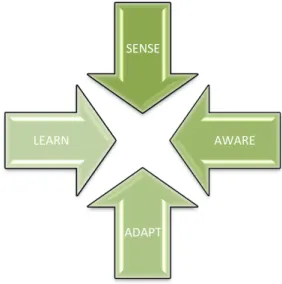
Cognitive Radio (CR) is a model for radio communication in which a wireless system alters its transmission or reception to effectively communicate with end user avoiding interference from other users present in the spectrum [10]. CR continuously learns about the radio spectrum by sensing the spectrum and changes its transmission or reception parameters according to the user behavior. The spectrum sensing principals of cognitive radio is shown in Figure 2.1.

Figure 2.1 Cognitive Radio spectrum sensing

CR finds the free spectrum holes in the available spectrum range through sensing and learning. CR adapts to the changes in available radio spectrum and varies transmit or receive parameters according to the network condition. In the CR paradigm, there are two types of users known as Primary Users (PU) and Secondary Users (SU). Primary users are the licensed spectrum users who have direct access to the network whereas SUs are the users who rely on the CR decision for spectrum access [18]. There are two main types of spectrum sensing CRs

1. Licensed Band Cognitive Radios (LBCR): In which CR is capable of using licensed frequency bands assigned to users [10].

2. Unlicensed Band Cognitive Radios (UBCR): Which can only make use of the unlicensed part of Radio Frequency (RF) spectrum [10].

The rest of the discussion in this thesis focuses only on the second category of Cognitive Radios referring to it as CR.

SENSE

AWARE

ADAPT LEARN

(15)

2.1 Cognitive Radio Operation

CR emerged as an answer to spectrum crowding problem. Any CR‟s operation comprises of four states as shown in the Figure 2.2. First the available spectrum is sensed and analyzed to find any available spectrum holes. On the basis of spectrum analysis a decision is made to opportunistically assign the available frequency to the secondary user. Spectrum sensing is the most integral part of CR because all the remaining operations of CR rely on precise sensing of available spectrum [18].

Figure 2.2 Cognitive Radio operation

2.2

Types of Spectrum Sensing

The most important task of spectrum sensing is transmitter detection. Spectrum sensing plays a key role in the decision making part of CR. There are several different ways to sense the spectrum. Some of the key methods used for spectrum sensing are as follows:

1. Energy Detection 2. Cyclostationary Method 3. Matched Filter detection 4. Wavelet detection

Explanation and comparison of all four methods is given below.

Radio

Environment

Spectrum

Sensing

Spectrum

Analyzing

Spectrum

Decision

(16)

2.2.1 Energy Detection

In energy detection method we measure the energy of available radio resource and compare it against a predefined threshold level. If the measured energy falls below the defined threshold level spectrum is marked as available. When the measure energy level is above the defined threshold, it‟s considered as occupied. Energy detection method does not require any prior information of the signal. In simple words it does not care about the type of modulation used for transmission of signal, phase or any other parameter of signal. It simply tells if the radio resource is available at any given time instant or not without considering the PU and SU [10]. Hypothetically, energy detection can be considered as a method based on binary decision, which can be written as follows:

𝒙 𝒕 = 𝒏 𝒕 𝑯𝟎 (1) 𝒙 𝒕 = 𝒔 𝒕 + 𝒏 𝒕 𝑯𝟏 (2)

Where s(t) is the received signal and n(t) is the Additive White Gaussian Noise (AWGN) i.e. equally distributed all over the signal. H0 and H1 represent the two outcomes of the energy detection method [4]. The energy detection method‟s working principal can be explained with the Figure 2.3

Fast Fourier Transform Windowing the Peak FFT Magnitude X(t) X(f) Y(f) Decide H0 or H1

Figure 2.3: Energy Detection method

2.2.2 Cyclostationary Method

A Cyclostationary process is defined as the statistical process which repeats itself cyclically or periodically [6]. Communication signals are Cyclostationary with multiple periodicities. Mathematically Cyclostationary detection can be performed as given in equation (3):

𝑹𝒙 𝑻 = 𝑬 𝒙 𝒕 + 𝑻 𝒙∗_{𝒕 − 𝑻 e}−j2απ t₍₃₎

The equation shows the autocorrelation of the observed signal x(t) with periodicity T, E represents the expectation of the outcome and α represents the cyclic frequency [6]. After autocorrelation Discrete Fourier Transform over resulting correlation is performed to get the desired result in terms of frequency components. The peaks in the acquired data give us the information about the spectrum occupancy. The Cyclostationary detection method requires prior

(17)

knowledge of periodicity of signal and it can only be used with the signal possessing Cyclostationary properties. The implementation of Cyclostationary method is shown in Figure 2.4.

FFT Correlation of _{x(f+α)x*(f-α)} Cyclic freq.

Detector

X(t) X(f) _S(f,α) Decide H0 or H1

Figure 2.4: Cyclostationary Detection [10]

2.2.3 Matched filter detection

In the matched filter detection method a known signal is correlated with an unknown signal captured from the available radio resource to detect the presence of pattern in the unknown signal [6]. Matched filter detection method is commonly used in Radio Detection and Ranging (RADAR) communication [10]. The use of matched filter detection is very limited as it requires the prior information about the unknown signal. For example in case of GSM, the information about the preamble is required to detect the spectrum through matched filter detection method. In case of WiMAX signal prior information about the Pseudo Noise (PN) sequence is required for detection of spectrum.

2.2.4 Wavelet Detection

To detect the wideband signals, wavelet detection method offers advantage over the rest of the methods in terms of both simplicity and flexibility. It can be used for dynamic spectrum access. To identify the white spaces or spectrum holes in the available radio resource, the entire spectrum is treated as the sequence of frequency sub-bands. Each sub-band of frequency has smooth power characteristics within the sub-band but changes abruptly on the edge of next sub-band. By using the wavelet detection method the spectrum holes can be found at a given instance of time by finding the singularities in the attained result [10]. The Figure 2.5 shows the wavelet detection implementation for spectrum sensing. Fast Fourier Transform Power spectral density of X(f) magnitude Local maximum Detection X(f) _S(f) Decide H0 or H1 X(t)

(18)

2.3 Qualitative analysis of spectrum sensing techniques

All of the above mentioned spectrum sensing techniques have certain advantages and disadvantages. Some of the techniques are suitable for sensing of licensed spectrum whereas others are suitable for unlicensed spectrum. The qualitative analysis of above mentioned spectrum sensing techniques are presented in Table1.

Table1. Spectrum sensing techniques comparison

Sensing technique Advantages Disadvantages

Energy Detection Does not require prior

information, Efficient, less complex

Limited functionality in low SNR areas, cannot differentiate between PU and SU

Cyclostationary Works perfectly in low

SNR areas, robust against interference

Requires fractional information about the PU, less efficient in terms of computation cost

Matched Filter Low computation cost,

accurate detection

Requires prior information about PU

Wavelet Detection Works efficiently for

wideband signal detection

Does not work for DSSS, more complex

It can clearly be seen from table1 that energy detection is the most suitable technique for unlicencessed spectrum bands as it does not require any prior information about the PU and SU.

2.4 Radio spectrum overview

Radio spectrum comprises of electromagnetic frequencies ranging lower than 30 GHz or having wavelength larger than 1milimeter (mm). Various parts of the radio spectrum are allocated for different kinds of communication application varying from microphones to satellite communication. Today, in most of the countries radio spectrum is government regulated i.e. governments and some other governing bodies like International Telecommunication Union (ITU-T) assign the radio spectrum parts to communication services [1].

There are several different frequency bands defined inside the radio spectrum on the basis of wavelength (λ) and frequency (f). Generically radio spectrum can be classified into two categories as licensed spectrum and unlicensed spectrum. Licensed spectrum comprises of frequency bands governed by government regulated agencies. It is illegal to use licensed frequency spectrum without taking permission from the regulatory bodies. Unlicensed frequency bands can be used by anyone for any scientific or industrial research.

(19)

One of the known unlicensed frequency band is Industrial, Scientific and Medical (ISM) frequency band or spectrum. It comprises of several different frequency bands. The ISM band defined by ITU-Regulation is given in the Table2.

Table2: ITU-R allocation of ISM Frequency bands [10]

Frequency Range Center Frequency Availability

6.765-6.795 MHz 6.785MHz

13.553–13.567 MHz 13.560 MHz

26.957–27.283 MHz 27.120 MHz

40.66–40.70 MHz 40.68 MHz

433.05-434.79 MHz 433.92 MHz

902-928 MHz 915 MHz ITU Region2 only

2.400-2.500 GHz 2.450 GHz 5.725-5.875 GHz 5.800 GHz 24-24.25 GHz 24.125 GHz 61-61.5 GHz 61.25 122-123 GHz 122.5 GHz 244-246 GHz 245 GHz

Most commonly used ISM bands are 2.4 GHz and 5.8 GHz band. Though these ISM bands were reserved for the purpose of research but currently these bands are used for different wireless communication standards. Examples of these bands are Wireless Local Area Network defined by Institute of Electrical and Electronics Engineers (IEEE) as 802.11a/b/g/n, Wireless Personal Area Network (WPAN) defined by IEEE as 802.15 and Cordless phones which operate in the range of 915 MHz, 2.4 GHz, and 5.8 GHz. The research carried out in this thesis is performed using the 2.4 GHz and 5.8 GHz ISM band commonly used for WLAN and defined by IEEE as 802.11. 802.11 standards have defined 13 channels in the range of 2412MHz to 2472MHz. Each channel is 5MHz apart from each other and all the adjacent channel overlap with each other as each channel is 22MHz wide as shown in Figure 2.6.

(20)

2.5 Related work

The recent focus on CR technology and advent of Software Defined Radio (SDR) such as GNU Radio has led to the implementation of GNU Radio in terms of the Cognitive Radio [3]. There are hundreds of citations available on IEEE explore investigating different aspects of spectrum sensing and CR. Most of the ongoing debate is concerned about finding the right spectrum sensing techniques for CR, channel allocation and transmission power handling for the Media Access Control (MAC) and Physical (PHY) layer implementation [5]. Underutilized bandwidth detection is key element of any spectrum sensing technique [9].

There are number of different platforms available for the implementation of CR in terms of SDR. One of these platforms include Open source Software Communication Architecture (SCA) implementation-Embedded (OSSIE) by Virginia Tech [24]. OSSIE is an open source software radio suite which can be used to model any of SDR and CR applications. Other platforms include High Power SDR (HPSDR) [25] and Flex Radio [26].

There are some other technique that could be considered as alternative to spectrum sensing. One of these techniques is cognition enabling pilot channel (CPC) [6]. According to CPC, a database of licensed users can be created which will monitor the use of spectrum by creating another channel and by advertising the spectrum opportunities in timely manner. But this will restult in additional infrastructure and use of another channel known as CPC. It is not the best approach to overcome spectrum scarcity as it will result in extra overhead in terms of radio resource.

(21)

CHAPTER 3

(22)

3 R

ESEARCH

M

ETHODOLOGY

This chapter presents the research methodology used to carry out the project under consideration. This thesis covers all parts of a standard research methodology approach starting from the problem identification to soluction and from implementaion to validation of results. We have used qualitative, quantitative analysis and experimental methods to answer the research problem under consideration.

The work started with the literature review of CR. Firstly a thorough study of cognitive radio paradigm was conceded. After getting acquainted with the working principles of CRs, through journals and research papers, we narrow downed the scope to a more specific area of interest i.e. spectrum sensing. Spectrum sensing was chosen because of it‟s key role in making CR realizable. A further refined search was carried out on spectrum sensing using IEEE explore website to get the knowledge about the current research in the area of spectrum sensing.. Furthermore we conducted meeting with our supervisor Mr. Alexenderu Popescu, Dr. David Erman and Mr. Yang Yao to get further insight into the problem. On the foundation of knowledge base collected over a period of time we defined our research questions. we made deductive and statistical hypothesis to answer the research question. To strengthen our defined hypothesis and to motivate our answer, we first figured out if there are any white spaces in the congested 2.4 GHz ISM band.

The most essential part of any CR is to find the underutilized bandwidth in available radio spectrum in an efficeint manner. The underutilized bandwidth or spectrum holes should be found with the minimal information about spectrum as it is difficult to consider all the dimensions of radio spectrum while monitoring the spectrum for spectrum holes. Study about the all the available spectrum sensing techniques was carried out in terms of qualitative analysis. For experimental and quantitative analysis we used a testbench called USRP2 and GNU Radio which is an FPGA board with RF transciever interfaced with a Linux PC carrying GNU Radio software also known as Software defined Radio (SDR). Firstly we found out which technique of spectrum sensing is most robust for ISM bands.

After conducting a qualitative research, we found that energy detection method and wavelet detection method was most approperiate for the problem underconsideration. We implemented the algorithem over the testbench and gathered the results in forms of raw data constituting FFT values of spectrum at different instances of time. The data collected in real time was arranged in tables so that results could be monitored in graphical way. We conducted the

(23)

experiments for both 2.4 GHz and 5.8 GHz ISM band. One of the major task was to present the data in a grpahical manner so that all three dimensions i.e., frequency, time, gain could be taken underconsideration at the same time. For this purpose, we developed spectrograms and 3D-plots to get a clear understanding of outcome and to validate the results in comparison to the hypothesis under consideration. The results and experiments are presented in the next section.

(24)

CHAPTER 4 GNU Radio and Universal

Software Radio Peripheral 2

(25)

4 GNU

R

ADIO AND

USRP2

4.1 GNU Radio Overview

GNU Radio is an open source development platform for signal processing and communication applications focusing on implementation of SDRs with low cost external RF hardware. It contains tons of libraries with signal processing routines written in C/C++ programming language. It is widely used in the wireless communication research and real time implementation of software radio systems [16].

GNU Radio applications are mainly written and developed by using Python programming language. Python provides a user friendly frontend environment to the developer to write routines in a rapid way. The performance critical signal processing routines are written in C++ [22]. Python is a high level language; it acts as a glue to integrate the routines written in C++ and executes through python. Python uses simplified wrapper and interface grabber (SWIG) for the purpose of interfacing C++ routines with python frontend application as shown in Figure 4.1. Very high speed integrated circuits hardware description language (VHDL) is a hardware descriptive language. This part of the code is executed in the Field Programmable Gate Array (FPGA) of front end hardware which is USRP2 in our scenario.

VHDL/Verilog FPGA

Python glue C++ C++ C++ C++ C++ SWIG Signal Processing Blocks

(26)

GNU radio applications can be developed using both Object Oriented Approach and Procedural Approach depending upon the complexity of the problem under consideration. Some of the modules available in the current release of GNU Radio are shown in Figure 4.2:

Figure 4.2: GNU Radio Modules [22]

4.1.1 GNU Radio Flow graphs, Sources and Sinks

Any GNU Radio application can be presented as a collection of flow graphs as in graph theory. The nodes of such flow graphs are called processing blocks. Processing blocks are the code routines written in C++. These processing blocks are tied together through flow graphs or lines connecting blocks. Data flows from one block to another through these flow graphs. All data types which are available in C++ can be used in GNU Radio applications e.g. real or complex integers, floats, etc [22]. Each block connecting one end of flow graph performs one signal processing operation for example encoding, decoding,

(27)

hardware access etc. Every flow graph in GNU Radio requires at least one source or sink. Source and Sinks can be explained with the example of spectrum sensing scenario explained later in this chapter. In case of spectrum sensing our command line interface acts as sink whereas USRP2 acts as a source. When we use input command line parameters to tune USRP2 in this scenario, the interface acts as a source and USRP2 acts as a sink.

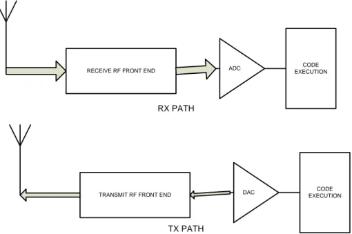
4.2 Typical Software Radio

A typical software radio consists of RF front and Analogue to Digital Converter (ADC) and Digital to Analogue Converter (DAC) interfaced with Central Processing Unit (CPU) and software. Receive and transmit path of typical software radio is shown in Figure 4.3:

RECEIVE RF FRONT END ADC EXECUTIONCODE

TRANSMIT RF FRONT END DAC

CODE EXECUTION

RX PATH

TX PATH

Figure 4.3: Basic Software Radio

4.3 USRP2 Architecture and Overview

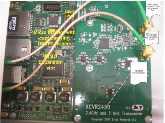
USRP2 allows the creation of a software radio with any computer having gigabit Ethernet interface. It‟s the upgraded version of its earlier release USRP. USRP has a USB interface limiting the data throughput from USRP to Computer at a maximum bandwidth of 8MHz. The design of USRP and USRP2 is open source and all schematics and component information can be downloaded from the website of the manufacturer [2]. USRP2 contains field programmable gate arrays (FPGA) and RF transceiver board which is

(28)

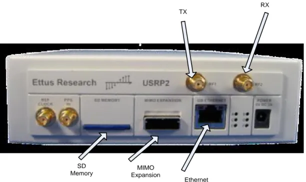
The main idea behind the design of USRP is to perform all the signal processing tasks for example modulation and demodulation, filtering at the host computer. All the general purpose tasks such as decimation, interpolation, digital up conversion and down conversion are performed inside the FPGA of USRP2. The Figure 4.4 shows the image of USRP2 with RF daughter board. USRP2 contains gigabit Ethernet controller, SD card slot and MIMO expansion slot at the front end with 8 LED indicators. SD card contains the driver for USRP2 mother board and RF transceiver. It requires 5V DC and 6A to power up USRP2 [2]. The main features of USRP2 are given in table 3.

(29)

SD

Memory _ExpansionMIMO

Ethernet Interface TX

RX

Figure 4.5: USRP2 Front end Table 3: Main features of USRP2

Interface Gigabit Ethernet

FPGA Xilinx Spartan 3 2000

RF Bandwidth 25MHz ADC 14 bits, 100MS/s DAC 16 bits, 400 MS/s Daughterboard slots 1 Tx, 1 Rx SRAM 1 MB Power 5V DC, 3A

4.3.1 USRP2 Operation with GNU Radio

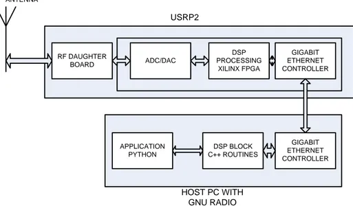
USRP2 operation with GNU Radio can be explained with the help of Figure 3.6. RF transceiver fetches the RF signal from real time environment and converts it to Intermediate Frequency (IF) around direct current (DC). After converting it to IF the signal is passed to ADC. USRP2 contains two 14-bit ADC which provides sampling rate of 100MS/s [2]. The ADC after sampling passes the data to FPGA. The main task for the FPGA is the down conversion of remaining frequency and data rate conversion. After processing, FPGA transfers the results to gigabit Ethernet controller which passes it over to the host computer where the rest of the signal processing tasks are performed.

(30)

USRP2. After receiving, the complex signal, digital up converter (DUC) converts the signal to IF before passing it to DAC. The DAC passes the IF converted signal to the RF transceiver where it is converted to RF signal and transmitted over the air.

RF DAUGHTER BOARD ADC/DAC DSP PROCESSING XILINX FPGA GIGABIT ETHERNET CONTROLLER APPLICATION PYTHON DSP BLOCK C++ ROUTINES GIGABIT ETHERNET CONTROLLER ANTENNA USRP2 HOST PC WITH GNU RADIO

Figure 4.6: USRP2 operation with GNU Radio

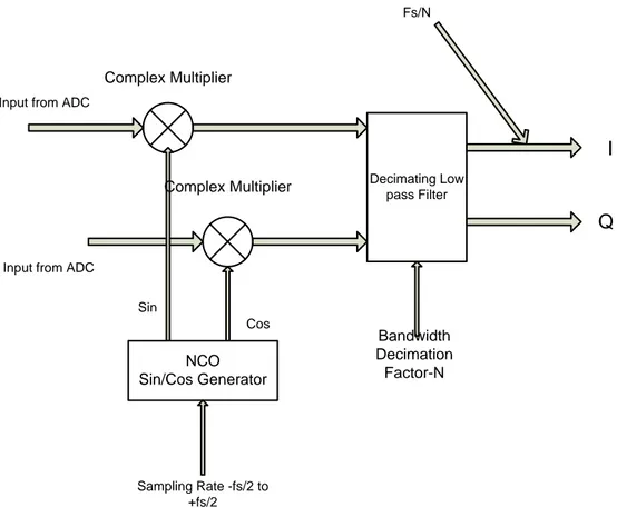
In the FPGA down conversion of the signal from IF to baseband is performed. The data rate is further reduced so that it can be tailored according to the performance of transmission interface. The function of DDC in FPGA is as described in figure 4.7. The complex IF input signal is multiplied with the Numerically Controlled Oscillator (NCO). The signal resulting from the multiplication with the frequency of NCO is also complex and centered at DC. The process is similar to the one used in heterodyne receivers. The signal is then decimated with the factor N to further adjust the sampling rate. The phase generator in NCO is clocked at 125 MHz. The clock can be adjusted numerically or can be adjusted from the interface as well. The decimation factor is fed to the system through the gigabit Ethernet interface. The I and Q lines carry 16-bit signed integers through the gigabit Ethernet interface making each I and Q sample 4 bytes wide respectively. USRP2 is capable of

(31)

NCO Sin/Cos Generator Decimating Low pass Filter Complex Multiplier Complex Multiplier Bandwidth Decimation Factor-N

Input from ADC

Sampling Rate -fs/2 to +fs/2 Fs/N I Sin Cos Q

(32)

CHAPTER 5 Energy detection implementation

using USRP2 and GNU Radio

(33)

5 E

NERGY DETECTION IMPLEMENTATION USING

USRP2

AND GNU RADIO

5.1 Project Setup

The project setup was created by using GNU Radio installed on Ubuntu Linux 10.10 on personal computer (PC) with the specifications; core 2 Duo, 4 GB ram, 320 GB hard drive, Gigabyte Ethernet interface and ATI Radeon 512 MB graphics card. USRP2 device was used to physically receive the signal from real time environment. The USRP2 was connected to the Ethernet port of Host PC gigabit Ethernet card through CAT6 cable carrying RJ-45 jack at both ends. The USRP2 differs from its predecessor in a way that it requires certain configurations for boot up process unlike USRP which connects through USB port. It requires certain configuration at Linux terminal to make it work with GNU Radio. First the drivers were updated for USRP2 with XCVR2450. Universal Hardware Devices (UHD) provides complete support for the drivers of USRP2 product line. UHD provides both host drivers and Application programming Interface for standalone application development without GNU radio suite. USRP2 communicates at IP/UDP layer. The default IP address for USRP2 is 192.168.10.2, so to make it work Host PC should be assigned an IP address in the same subnet, for example 192.168.10.1. When USRP2 is not assigned an IP address, it communicates with the host pc using UDP broadcast packets, so it is essential to turn off the firewall before establishing the connection with USRP2 [2]. USRP2 can be found on the terminal by entering the following command provided by UHD.

$ sudo find_usrps

00:50:c2:85:35:14 hw_rev = 0x0400

The command returns the MAC address of the USRP2 showing it is available and connected to the interface. GNU radio provides a python routine named USRP2_probe.py which acts as a software RF probe. It is a graphical user interface (GUI) application which returns the frequency range for the transceiver board and its gain in milliWatt-decibel (dBm). The output of the USRP2_probe.py for XCVR2450 dual band transceiver is given in Figure 5.1.

(34)

Figure 5.1: USRP2_probe.py Output

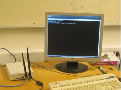
After connecting the USRP2 with GNU radio and bringing it to up and running condition now we can execute any GNU Radio application by writing a routine in python or by using GNU Radio Companion (GRC). The experimental setup is shown in Figure 5.2 :

Figure 5.2: Experimental Setup

In this project we developed a routine called USRP2_spectrum.py which is based on usrp_spectrum_sense.py a standard routine available in GNU Radio latest release. The routine works as a software spectrum analyzer and is flexible enough to monitor any RF spectrum. The routine provided in GNU radio libraries was written for USRP first release and has certain limitation in terms of data rate and bandwidth due to USB interface of USRP. It can only monitor a maximum of 8MHz bandwidth at any

(35)

given time whereas USRP2 has a gigabit Ethernet making it flexible enough to monitor the 25MHz of bandwidth at any given time [2]. Hence we modified the routine to make it work with the USRP2.

There are some other routines (written in python) available in GNU Radio but none of these routines are flexible enough to monitor the whole spectrum for a long interval of time. One of these routines is USRP2_fft.py. This is a GUI application which takes the FFT of the received signal in real time and displays it over interface. The limitation with USRP2_fft.py is that, it only provides us with the gain at a given frequency without displaying the spectrum holes. Secondly it is a GUI application and it can only be executed using a low decimation rate, otherwise system specs should be very high. The output of the USRP2_fft.py is shown in Figure 5.3 showing the utilization of channel 1 of 2.4 GHz ISM band in BTH, Karlskrona Campus.

Figure 5.3: USRP2_fft.py output

Similarly, there is another application USRP2_rx_cfile.py. The application works as a broad band receiver, it fetches the signal from the external source environment and dumps the Digital down converter output in form of I and Q data directly into the appended file. The data collected at particular time t can be plotted using another GNU radio application named gr_plot_fft.py. The gr_plot_fft.py plots the raw data collection in terms of FFT as shown in Figure 5.4. USRP2_rx_cfile.py has a limitation in terms that it can only extract the data for a given center frequency as shown in Figure 5.4. The Figure show the utilization of RF spectrum at 2.437 GHz i.e. channel 6 of 2.4 GHz ISM band.

(36)

Figure 5.4: gr_plot_fft.py output with USRP2_rx_cfile.py data file The modified spectrum sensing routine implemented by us overcomes the deficiencies which we have mentioned in available standard routines.

5.2 Spectrum sensing Algorithm implementation

Implementation of spectrum sensing algorithm can be explained with the help of flow graph presented in Figure 5.5. Flow chart shows the flow of data from source i.e., USRP2 to SINK which is Linux command line interface in our scenario. Source i.e. USRP2 fetches the signal of the desired frequency passed to it as a tuning parameter. After passing through USRP2 the raw data bit streams are converted to vectors or arrays of data. FFT is performed on the received raw data with the help of signal processing blocks and it is passed through the Blackman-Harris window to overcome the spectral leakage effect. When the FFT routine is implemented on a non periodic data, it results into spectral leakage i.e. the energy of the signal spreads out to a larger band of frequencies. Window functions helps out in reducing the effect of spectral leakage. After performing the FFT magnitude, decimation of the data is performed. Decimation is the inverse of interpolation. Decimation reduces the sample rate of data by performing down sampling to the desired rate and send to USPR2 as a tuning parameter. After performing decimation the obtained data is appended into a file or it can be plotted on the go through a GUI tool. The data collected is in the form of FFT magnitude bins. By plotting these magnitude bins against the given frequency range the frequency envelop of the signal can be monitored to find the white spaces or spectrum holes. By taking

(37)

the Power Spectral Density of received FFT magnitude bins we can use the same algorithm for wavelet detection method.

USRP2 SOURCE Bit stream to Vector Conversion FFT Magnitude Decimation Sink Tunning Parameter Blackman-Harris window

Figure 5.5: USRP2_spectrum.py flow chart

The spectrum sensing algorithm steps across the RF spectrum and takes the measurement in terms of FFT magnitude bins. The number of FFT bins, gain, decimation, time delay, dual delay and frequency range are forwarded to the USRP2_spectrum.py as tuning parameters.

The minimum number of bins is 3 and the maximum is 1024 bins. The FFT magnitude bins received at a certain frequency consist of 2 parts. First half of the bins i.e. FFT X[1] to FFT X[N/2 - 1] corresponds to the pass band spectrum from the center frequency (fc) to +Fs/2. Whereas the rest of the bins from X [N/2 - 1] to X [N-1] contains spectrum from center frequency to –Fs/2. Here X[1] represents the first bin value as shown in appendix B and X[N/2 - 1] represents the middle bin value. For example if we have 256 bins at 2402 MHz with 8MHz frequency step, the bin 0 to 127 corresponds to 2398 MHz to 2402 MHz and the rest of the bins correspond to 2402 MHz to 2406 MHz.

The gain parameter sets the gain of tuner card. By default the gain of the card is set to half of maximum gain which is 45dBm in case of XCVR2450. The time delay and dual delay parameters depends upon the decimation rate and length of FFT. By default decimation rate is set to 16 with 256 FFT bins and with time delay of 1ms. Time delay is a key parameter without setting the correct time

(38)

forwarded in the defined time. Time delay for a given decimation rate and FFT size can be calculated as follows:

No. of FFT Frames = (Decimation Rate * Time delay) / FFT window Size (4) In practice to reduce the non linear response of the DDC we performed FFT overlapping. Without FFT overlapping we were getting white spaces at the end of every sweep. We choose an overlap minimum of 25% i.e. we defined the step size to 8MHz for every step. In some cases we even choose overlapping of 0.75% to get the step size of 1MHz, so that we can get as accurate results as possible. The USRP2_spectrum.py is invoked in the following manner:

$ Sudo python USRP2_spectrum.py –a2.4G –b2.5G –g45 –d8 >rx.dat The time delay parameter is set to 1ms in the code by default. –a represents the starting frequency and –b represents the last frequency, -g is used to set the gain parameter and-d8 represents that we are using decimation of 8.Decimation rate of 8 means that USRP2 processed(100MS/s divided by 8 i.e., Fs/N) 12.5MS/s during execution of code. The USRP2_spectrum.py is provided in appendix A at the end of the thesis. The typical output of running USRP2_spectrum.py will give us the FFT magnitude bins at a given center frequency. The gain at any given center frequency can be calculated by summing the values of all the bins and by taking square root of the result. After that by taking 20*log(x), where x is the square root of the sum of the bins, we can get the result in dBm.

The experiments were carried out in Room G403 of Building2 at Blekinge institute of technology (BTH) in Karlskrona, Sweden. Most of the results were collected during the same project room except a few instances where the results were collected in the cafeteria while turning on the microwave to check the performance of the algorithm in presence of high noise.

5.3 Project Limitations

Project limitations can be classified into two categories i.e.  Hardware limitations

 Energy Detection Algorithm limitations

5.3.1 Hardware Limitations

The results were attained using decimation rate of 8.i.e 12.5MS/s. More precise results can be obtained by using lower decimation value. USRP2 can monitor maximum bandwidth of 25MHz. The receiver sensitivity can be increased by using a high gain antenna with the tuner card.

(39)

5.3.2 Energy detection Algorithm limitations

As previously mentioned energy detection based algorithms cannot differentiate between PU and SU [11]. The results are solely based on the threshold level received, or the energy level measured from the environment. Energy detection method cannot be used in a low noise setup. The implemented routine can sense large bandwidth but not at the same time as it steps across the RF spectrum with the change in time domain.

(40)

CHAPTER 6 Results

(41)

6 R

ESULTS

The raw data collected by executing the USRP2_spectrum.py routine is appended into .dat and .bin files. These file can be loaded directly into MATLAB or any other plotting tools like octave, SigView or wavelet toolbox software. All the results in this chapter are plotted using Matlab2010 and Sigview. The sample raw data extracted in the „.dat‟ file is shown in appendix B. The results obtained show the usage of 2.4 GHz WiFi channels in the campus as well as free channels and spectrum holes. The results are collected using both 2.4 GHz ISM band and 5.8 GHz ISM band. The 5.8 GHz band is not used within the campus environment which can easily be observed by looking at frequency and magnitude plot. We have used three different types of plots to verify our results. These are frequency, magnitude and time, frequency, gain 3-dimensional (3D) plots and time, frequency spectrograms.

Figure 6.1 shows the results obtained for 2.4 GHz ISM band by using a frequency step of 20MHz i.e. the above defined routine steps across the ISM band in steps of 20MHz starting from 2.4 GHz and ending at 2.502G. As it can be observed from the graph, it is hard to find the exact channel utilization of 802.11 WiFi spectrum due to large sweeps across the spectrum. The Figure 6.1 shows first three cycles of algorithm i.e. algorithm steps across the spectrum in 5 steps in case of 20 MHz. Figure 6.2 shows the step plot with 20MHz step but it shows the results for a longer period of time which can be seen from the marking on the stems. The main purpose of continues and stem plot is to simply monitor the gain of the sensed signal at a particular frequency. These two dimensional plots simply tells us about the utilization of WLAN channels in BTH network. Figure 6.3 shows the same results in 3-dimensions (3-D) by using another axis for time. The advantage of time axis is that we can monitor the results at any given instance of time. The time dimension gives us flexibility to find the white spaces or spectrum holes in radio spectrum at any given instance of time t. Figure 6.3 shows the results in terms of Frequency, Gain (dBm), and time. The gain factor is calculate by dividing received samples by total number of bins and by taking log of FFT magnitude values as given in appendix C. The gain factor tells us that the signal strength has increased by a certain factor as compared to the original signal or other comparative signal samples depending upon the scenario.

(42)

Figure 6.1: FFT magnitude plot for 2.4 GHz band with 20 MHz frequency Step

Figure 6.2: Frequency vs. FFT magnitude stem plot for 2.4-2.5 GHz ISM band

(43)

Figure 6.3: Time, Frequency, and Gain 3D plot for 2.4 GHz-2.5 GHz using 20 MHz frequency step

The results obtained using a smaller step of 10MHz is shown in Figure 6.4. We can easily find the channel utilization of campus WLAN by looking at Figure 6.4 and Figure 6.5. The spikes around 2.43x109 Hz in the plot show the use of Channel 7 at the time of data collection. Frequency and magnitude plots provide us gain at a given frequency but still it‟s not good enough to find the threshold level or to decide which part of spectrum is free because it does not has the time-axis. For this purpose we have used spectrograms.

(44)

Figure 6.5: Frequency and Magnitude plot with 10 MHz step at 2.4 GHz ISM band

Figure 6.6: Time, Frequency, Magnitude plot using 10 MHz step Spectrogram shown in Figure 6.7 displays the time frequency relationship with respect to gain. A spectrogram is a time varying spectral representation of a signal which shows how the spectral density of the signal varies with time. The color bar presented at the right side of the plot shows the different level of energy or gain values. To find the spectrum holes or availability at the defined threshold at any instant, we can compare the color with time and frequency axis. The color red in this

(45)

Figure 6.7: Spectrogram plot using 10 MHz step

Spectrogram shows the spectrum holes or underutilized bandwidth at a given instance of time and Frequency. Due to large frequency step it is hard to differentiate between the colors and it is hard to find the white spaces at the exact location.

To gather even more precise results we repeated the experiment with 5 MHz frequency step and sweep across the spectrum again. The results obtained are shown in Figure 6.8-6.10. Here we can easily observe the use of channel 3,7,11 in the campus WLAN environment by looking at Figure 6.8 and Figure 6.9. each stem value represents the results collected during separate cycle of data collection presented collectively in one stem plot. The utilization of channel 3,7,11 is expected as at these channel frequencies we have the maximum gain values at a given instance of time t.

(46)

The spectrogram given in Figure 6.10 is more precise in terms of clarity showing spectrum holes in terms of red tiled surface in the presence of other colors representing different gain values of energy spectrum. the better results are attained by using a lower frequency resolution or step size which is 5 MHz in this case.

Figure 6.9: Time, Frequency, gain 3D plot with frequency step of 5MHz

(47)

Similarly we gathered the results using 1MHz step. The results obtained are shown in Figure 6.11 and Figure 6.12 showing the utilization of channel 1, 7 and 11 in the WiFi network of the campus.

(48)

To check the limitations of our project we conducted another experiment by placing the USRP2 and host PC near microwave ovens to check if energy detection method is susceptible to the high signal strength environment or not. The results attained are shown in Figure 6.13, 6.14 and 6.15. The results clearly show increase in gain in less than 1 second. We received gain values as high as 50dBm and energy detection algorithm didn‟t identify any other WiFi channel though the university café is a hotspot and it has a number of wireless routers placed in the vicinity. The spectrogram in Figure 6.15 shows the use of only microwave oven frequency i.e. 2.45 GHz in different colors the rest of the frequency range is red proving microwave frequency magnitude to be high enough to suppress any other signal in the vicinity of cafeteria.

(49)

Figure 6.14: Time, Frequency, Gain 3D plot at microwave oven frequency

Figure 6.15: Spectrogram for microwave oven frequency .

(50)

Figure 6.16: Frequency vs. gain plot for 5.8 GHz ISM band

(51)

Figure 6.18: Spectrogram for 5.8 GHz ISM band

Final experiment was conducted over 5.8 GHz ISM band. Since 5.8 GHz frequency band is not used inside the campus, the whole spectrum range appears as white space or underutilized. It can be observed by looking at the Figure 6.17-6.18. A few colored spots in the spectrogram are due to the thermal noise or other hardware noise figure.

(52)

CHAPTER 7

(53)

7 C

ONCLUSION AND

F

UTURE WORK

The report presents implementation of energy detection and wavelet based spectrum sensing implementation and analysis of different spectrum sensing techniques. Different experiments were performed to find out the spectrum holes in the occupied 2.4 GHz ISM band. The raw data collected by USRP2_spectrum.py is plotted using different plotting techniques to find the spectrum holes. The qualitative analysis of different spectrum sensing methods shows that energy detection is the most reliable and authentic method for the spectrum sensing as it has the lowest computational cost and requires no a prior information about the spectrum. The raw data collected in the form of FFT bins is the most efficient way of collecting data for spectrum sensing as it requires just a few signal processing operations. Rest of the work is performed inside the USRP2, This is closest one can get to the hardware for precise results. The results obtained proved that it is possible to find the underutilized bandwidth in a spectrum without having prior knowledge of PU and SU. Spectrograms though often used in astronomy and acoustics can be used to identify the spectrum holes as shown in the result by plotting spectrograms. The threshold level for any given spectrum of frequencies depends upon several factors such as receiver sensitivity and the number of energy transmitting/receiving nodes and the dimensions taken under consideration.

7.1 Future work

Cognitive radio is relatively new area of research as compared to the rest of communication theory. There are several other methods of spectrum sensing which need to be explored. Energy detection method results can be improved through the use of the Multiple Input Multiple Output (MIMO) approach. This can be done by connecting multiple USRP2 together and sensing the spectrum for a large area. Another way to sense the spectrum is by using cooperative communication and by taking antenna diversity and other factors under consideration. This study could be extended by repeating the same experiment for licensed frequency bands and the results obtained can be compared with ISM band results to get the better understanding of the area of research.

(54)

Bibliography

[1] J.Mitola. “Software radios-survey, critical evaluation and future directions”,

IEEE National Telesystems Conference, pages 13/15- 13/23, 19-20 May 1992.

[2] Matt Ettus. Universal software radio peripheral. http://www.ettus.com.

[3] T. Yucek and H. Arslan, “A survey of spectrum sensing algorithms for cognitive radio applications,” IEEE Communications Surveys & Tutorials, vol. 11, no. 1, First Quarter 2009.

[4] M. Sarijari, A. Marwanto, “Energy detection sensing based on GNU radio and USRP, An analysis study”, 2009 IEEE 9th Malaysia International Conference on

Communications (MICC), no.15-17, pp.338-342, Dec. 2009.

[5] Shent, B.; Huang, L.; Zhao, C.; Zhou, Z. & Kwak, K. “Energy Detection Based Spectrum Sensing for Cognitive Radios in Noise of Uncertain Power”, Proc. Int. Symp. Communications and Information Technologies ISCIT 2008, 2008, 628-633 [6] End to End efficiency [E3] white paper, “Spectrum Sensing”, Nov. 2009.

[7] S. J. Shellhammer “Spectrum Sensing in IEEE 802.22,” Qualcomm Inc. 5755 Morehouse Drive San Diego, CA 92121, 2009.

[8] Pooyan Amini, Daryl Wasden, Arash Farhang, Ehsan Azarnasab, Peiman Amini, Behrouz Farhang-Boroujeny, “Cognitive spectrum assignment,” 2008 Software

Defined Radio Technical Conference and Product Exhibition, Oct. 26-30, 2008,

Washington D.C., Paper # 1.3-5. Conference Paper, published, 2008.

[9]. D. Cabric, A. Tkachenko, R. Brodersen, “Experimental study of spectrum sensing based on energy detection and network cooperation”, Proc. of the first international workshop on Technology and policy for accessing spectrum,2006. [10] Khaled Ben Letaief. "Cooperative Spectrum Sensing", Cognitive Wireless Communication Networks, 2007

[11] S. Haykin, “Cognitive radio: Brain-empowered wireless communications,” IEEE Journal on Selected Areas in Communications, February 2005.

[12] F. Penna, C. Pastrone, M. A. Spirito, and R. Garello, “Energy detection spectrum sensing with discontinuous primary user signal,” IEEE Proc. ICC, Jun. 2009.

(55)

[13] D. Cabric, A. Tkachenko, R. Brodersen, “Experimental study of spectrum sensing based on energy detection and network cooperation”, Proc. of the first international workshop on Technology and policy for accessing spectrum,2006. [14] H. Urkowitz, “Energy detection of unknown deterministic signals,” Proc. of

IEEE, pp. 523–531, Apr. 1967.

[15]. R. Tandra, A. Sahai, “SNR Walls for Signal Detection”, IEEE Journal of

Selected Topics in Signal Processing, vol.2, no.1, pp.4-17, Feb. 2008.

[16] GNURadio website, http://www.gnu.org/software/gnuradio/.

[17] Y. Zeng and Y. C. Liang, “Spectrum-sensing algorithms for cognitive radio based on statistical covariances,” IEEE Transactions on Vehicular Technology, vol. 58, no. 4, May 2009.

[18] J. Mitola and G. Q. Maquire, “Cognitive radio: making software radios more personal,” IEEE Pers. Commun.,Vol. 6, pp. 13–18, Aug. 1999.

[19] K. Arshad and K. Moessner, “Impact of User Correlation on Collaborative Spectrum sensing for Cognitive Radio,” in proc. ICT Mobile Summit 2009, 10-12 June „09, Satander, Spain.

[20] D.Cabric.S.M., Mishra.R.W., Brodersen, “Implementation Issues in Spectrum Sensing”, In Asilomar Conference on Signal, Systems and Computers, November 2004.

[21] Zhi Yan, Zhangchao Ma, Hanwen Cao, Gang Li, and Wenbo Wang, “Spectrum Sensing, Access and Coexistence Test bed for Cognitive Radio Using USRP”, 4th IEEE International Conference on Circuits and Systems for Communications, 2008. ICCSC 2008, 26-28 May 2008.

[22] GNURadio Wiki, http://gnuradio.org/redmine/wiki/gnuradio [23] Wikipedia, http://en.wikipedia.com

[24] SCA based open source software defined radio, http://ossie.wireless.vt.edu/ [25] High Performance Software Defined Radio (HPSDR), http://hpsdr.org/ [26] Flex Radio, http://www.flex-radio.com/

(56)

Appendix A

Code of USRP2_spectrum.py is written in python language. The modified part of the code is in italics. The rest of the code is taken from usrp_spectrum_sense.py which is a standard routine available in GNU Radio, and works for USRP first release only. There might be some indentation errors in the routine which can easily be fixed by copying the code in any standard python editor e.g. IDLE.

#!/usr/bin/env python

from gnuradio import gr, gru, eng_notation, window

from gnuradio import usrp2

from gnuradio.eng_option import eng_option from optparse import OptionParser

import sys import math import struct

class tune(gr.feval_dd): """

This class allows C++ code to call back into python. """

def __init__(self, tb): gr.feval_dd.__init__(self) self.tb = tb

def eval(self, ignore): try: new_freq = self.tb.set_next_freq() return new_freq except Exception, e:

print "tune: Exception: ", e

class parse_msg(object): def __init__(self, msg):

self.center_freq = msg.arg1() self.vlen = int(msg.arg2())

assert(msg.length() == self.vlen * gr.sizeof_float)

t = msg.to_string() self.raw_data = t

(57)

self.data = struct.unpack('%df' % (self.vlen,), t)

class my_top_block(gr.top_block): def __init__(self):

gr.top_block.__init__(self)

parser = OptionParser(option_class=eng_option)

parser.add_option("-e", "--interface", type="string", default="eth0", help="Select

ethernet interface. Default is eth0")

parser.add_option("-m", "--MAC_addr", type="string", default="", help="Select

USRP2 by its MAC address.Default is auto-select")

parser.add_option("-a", "--start", type="eng_float", default=1e7, help="Start ferquency [default = %default]")

parser.add_option("-b", "--stop", type="eng_float", default=1e8,help="Stop ferquency [default = %default]")

parser.add_option("", "--tune-delay", type="eng_float", default=10e-1,

metavar="SECS", help="time to delay (in seconds) after changing frequency [default=%default]")

parser.add_option("", "--dwell-delay", type="eng_float",default=100e-1,

metavar="SECS", help="time to dwell (in seconds) at a given frequncy [default=%default]")

parser.add_option("-g", "--gain", type="eng_float", default=None,help="set gain in dB (default is midpoint)")

parser.add_option("-s", "--fft-size", type="int", default=256, help="specify number of FFT bins [default=%default]")

parser.add_option("-d", "--decim", type="intx", default=16, help="set decimation to DECIM [default=%default]")

parser.add_option("-i", "--input_file", default="", help="radio input file", metavar="FILE")

(options, args) = parser.parse_args()

if options.input_file == "": self.IS_USRP2 = True else: self.IS_USRP2 = False self.min_freq = options.start self.max_freq = options.stop if self.min_freq > self.max_freq:

self.min_freq, self.max_freq = self.max_freq, self.min_freq # swap them print "Start and stop frequencies order swapped!"

self.fft_size = options.fft_size

# build graph

(58)

power = 0 for tap in mywindow: power += tap*tap

c2mag = gr.complex_to_mag_squared(self.fft_size)

#log = gr.nlog10_ff(10, self.fft_size, -20*math.log10(self.fft_size)-10*math.log10(power/self.fft_size))

# modifications for USRP2

if self.IS_USRP2:

self.u = usrp2.source_32fc(options.interface, options.MAC_addr) self.u.set_decim(options.decim)

samp_rate = self.u.adc_rate() / self.u.decim() else:

self.u = gr.file_source(gr.sizeof_gr_complex, options.input_file, True) samp_rate = 64e6 / options.decim

self.freq_step =0.75* samp_rate

self.min_center_freq = self.min_freq + self.freq_step/2

nsteps = math.ceil((self.max_freq - self.min_freq) / self.freq_step) self.max_center_freq = self.min_center_freq + (nsteps * self.freq_step) self.next_freq = self.min_center_freq

tune_delay = max(0, int(round(options.tune_delay * samp_rate / self.fft_size))) # in fft_frames

dwell_delay = max(1, int(round(options.dwell_delay * samp_rate / self.fft_size))) # in fft_frames

self.msgq = gr.msg_queue(16)

self._tune_callback = tune(self) # hang on to this to keep it from being GC'd stats = gr.bin_statistics_f(self.fft_size, self.msgq, self._tune_callback, tune_delay, dwell_delay)

self.connect(self.u, s2v, fft,c2mag,stats) if options.gain is None:

# if no gain was specified, use the mid-point in dB g = self.u.gain_range()

options.gain = float(g[0]+g[1])/2 def set_next_freq(self):

target_freq = self.next_freq

self.next_freq = self.next_freq + self.freq_step if self.next_freq >= self.max_center_freq: self.next_freq = self.min_center_freq if self.IS_USRP2:

if not self.set_freq(target_freq):

print "Failed to set frequency to ", target_freq, "Hz" return target_freq

(59)

return self.u.set_center_freq(target_freq) def set_gain(self, gain):

self.u.set_gain(gain) def main_loop(tb): while 1: m = parse_msg(tb.msgq.delete_head()) print m.center_freq print m.data . if __name__ == '__main__': tb = my_top_block() try:

tb.start() # start executing flow graph in another thread.. main_loop(tb)

except KeyboardInterrupt: pass

Spectrum sensing through implementation of USRP2