Application for Deriving 2D Images from 3D CT Image Data for Research Purposes

IN

DEGREE PROJECT TECHNOLOGY,

FIRST CYCLE, 15 CREDITS ,

STOCKHOLM SWEDEN 2016

Application for Deriving 2D Images

from 3D CT Image Data for

Research Purposes

NIELS AGERSKOV

This project was performed in collaboration with Karolinska University Hospital Supervisor at Karolinska University Hospital:Torkel Brismar

Application for Deriving 2D Images from 3D CT Image

Data for Research Purposes

Programvara för att härleda 2D-bilder från 3D CT

bilddata för forskningsändamål

Ni e l s A g e r s k o v

Ga b r i e l C a r r i z o

Degree project in medical engineering First level, 15 hp Supervisor at KTH: Lars-Gösta Hellström Examinator: Lars-Gösta

Hellström

School of Technology and Health KTH Royal Institute of Technology

Abstract

Karolinska University Hospital, Huddinge, Sweden, has long desired to plan hip prostheses with Computed Tomography (CT) scans instead of plain radiographs to save time and patient discomfort. This has not been possible previously as their current software is limited to prosthesis planning on traditional 2D X-ray images. The purpose of this project was therefore to create an application (software) that allows medical professionals to derive a 2D image from CT images that can be used for prosthesis planning.

In order to create the application NumPy and The Visualization Toolkit (VTK) Python code libraries were utilised and tied together with a graphical user interface library called PyQt4.

The application includes a graphical interface and methods for optimizing the images for prosthesis planning.

The application was finished and serves its purpose but the quality of the images needs to be evaluated with a larger sample group.

Sammanfattning

På Karolinska universitetssjukhuset, Huddinge har man länge önskat möjligheten att utföra mallningar av höftproteser med hjälp av data från datortomografiundersökningar (DT). Detta har hittills inte varit möjligt eftersom programmet som används för mallning av höftproteser enbart accepterar traditionella slätröntgenbilder. Därför var syftet med detta projekt att skapa en mjukvaru-applikation som kan användas för att generera 2D-bilder för mallning av proteser från DT-data.

För att skapa applikationen användes huvudsakligen Python-kodbiblioteken NumPy och The Visualization Toolkit (VTK) tillsammans med användargränssnittsbiblioteket PyQt4. I applikationen ingår ett grafiskt användargränssnitt och metoder för optimering av bilderna i mallningssammanhang.

Table Of Contents

3. Method and Material ... 5

3.1. Collection of Information ... 5

3.2. Material ... 5

3.3. Writing the Program ... 6

3.4. Compiling the Code ... 8

4. Results ... 9

4.1. Graphical User Interface ... 9

4.2. Derived Images ... 11

5. Discussion ... 14

5.1. Our programming choices ... 14

5.2. Resulting images ... 15

5.3 Programming software ... 15

5.4. Planning and time frame ... 16

5.5. Future work... 16

6. Conclusions ... 17

7. References ... 18 Appendix I: Images ... Appendix II: Relevant class references ...

1. Introduction

Hip fractures are one of the most common injuries in Sweden, with about 18,000 cases yearly. This is very resource demanding for the healthcare sector with costs of about 1.5 billion SEK yearly. The resource costs are a good reason for optimising each step in the treatment, imaging being one (Rikshöft, 2014, p. 7-9).

Considering the amount of examinations involving forms of x-ray, CT-scanning is the method that has seen the largest increase in usage. Between 1993 and 2010 the amounts of CT-scans in Sweden increased from 39 to 84 per 1000 inhabitants (Fäldt, Lindberg, 2013). This means that the amount of CT-data will also increase, which motivates the development of tools that can utilize this data, this application being one such tool.

When planning hip replacement surgeries at Karolinska University Hospital, Huddinge, a model of the prosthesis is created using a computer. Today and in the past this model has been done using traditional X-ray images because the software used for prosthesis planning at Karolinska University Hospital, only accepts X-ray images. In some cases the patient has already been scanned using a Computerised Tomography (CT) machine because of other injuries and this would be an excellent opportunity to capture images for hip modelling. Additionally, moving an injured patient between different machines can cause unnecessary pain and stress to the patient and also requires staff to chauffeur the patient around. Consequently, it would be more resource efficient and more comfortable for the patient if the hip prosthesis planning procedure could be performed using CT data instead of X-ray data (Brismar, 2016).

1.1. Objective

The main goal of the project was to create a prototype application software (in this report referred to as application). The application would be able to import a CT- volume, display it as a 3D-render, apply axial rotation and create a “simulated” radiographic image that can be used in hip prosthesis modelling.

To achieve the main goal the following subgoals needed to be reached: The application must be able to rotate a 3D-render of CT-data input. The application must be able to derive a 2D-image from 3D CT-data.

The derived image must be saved as a DICOM (Digital Imaging and Communications in Medicine, a standardised file format for medical imaging) image file with the appropriate DICOM tags, so that PACS and the planning tool accept the image.

1.2. Limitations

The project scope was limited in the following ways because of the software and material available at Karolinska University Hospital, Huddinge:

The application need to be designed to specifically work with the CT scanners available at Karolinska University Hospital, Huddinge.

The application has to be developed for use with Sectra’s PACS version 17.1.

2. Background

2.1. CT vs. CR

CT and traditional X-ray (also known as Computed Radiography or CR) are two medical imaging modalities. Both utilise gamma radiation and the way gamma rays interact with the body in order to construct an image of the inside of the body. The main difference between the two modalities is that traditional X-ray imaging is set up like a regular camera where the object is placed between the source and the detector. In CT, the source and the detector rotate around the object, which has been placed on a sliding bed, and capture multiple images along the body’s longitudinal axis. The CT images are often referred to as ‘slices’ and together the multiple slices make up a volume (Jacobson, 1995).

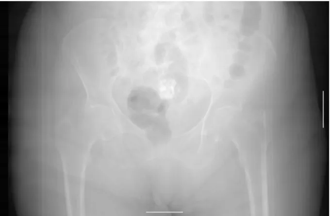
As with most technology, each modality has its advantages and disadvantages. CR images have high resolution but are static and usually noisy. Whether desired or not, an image is acquired of all the tissues in the part of the body chosen for examination and these tissues usually interfere with each other. In CT imaging different tissue types always have an attenuation (measured in Hounsfield units, HU) value in a specific interval range. This allows segmentation and manipulation of desired tissue types. For example, when evaluating bone tissue everything that has the same HU range as bone can be selected and evaluated separately (Jacobson, 1995). An example of a CR image (Image I.1) and a CT slice (Image I.2) can be found in Appendix I: Images.

2.2. Programming software

Python is a free, open source, dynamic programming language that is considered relatively simple in comparison to other popular programming languages. All code in this project has been written in Python version 2.7.11-0 (Python Software Foundation, 2016).

To be able to handle 3D rendering to a greater extent than Python allows for on its own, The Visualization Toolkit (VTK) was used. It is an open source code library that can be used in conjunction with Python (Kitware Inc.).

2.3. Object-oriented Programming

Object-oriented programming is programming around so-called “objects” and their states by manipulating the objects’ with logic sequences. These logic sequences are referred to as “methods”. For example, an image in this project has its’ state altered by for example a logic sequence (method) that rotates the image (Rouse, 2008).

2.4. PACS

PACS (Picture Archiving and Communication System) is a system that allows storing patient imaging data digitally. PACS also makes it possible to reach patient data from anywhere inside a hospital (Sectra, 2016).

2.5. Prosthesis planning

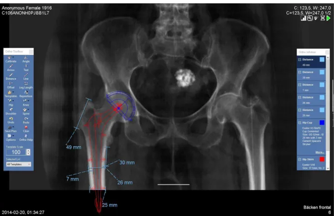
The modelling process at Karolinska University Hospital today is as mentioned in the introduction done with traditional radiographic images in 2D. In short it can be explained as: an image of the patients’ hip is taken using a traditional x-ray scanner. This image is then imported into the PACS. In the PACS a modelling software developed by Sectra called “Orthopaedic Solutions” can used by an orthopaedic surgeon. This is done by hand by dragging virtual prosthesis models onto the image earlier taken (Sectra, 2016). An example of a hip image with a prosthesis model applied can be seen below (Figure 2.5.1.).

3. Method and Material

The method section aims to explain the various parts that goes into the final application and how they were created. The completed application considered the actual objective of this project is presented in the results section.

3.1. Collection of Information

Initially, information was collected strictly to learn the basics of Python programming. For this purpose Python online tutorials, such as Tutorialspoint (2016) were utilised. VTK and NumPy were then explored mainly using PyScience. PyScience is a blog that among other things illustrates how Python can be utilised together with VTK to open, display and manipulate DICOM data (Kyriakou). For additional information about a library's classes, their official class and syntax documentation was consulted (see Appendix II: Relevant class references for URLs) General knowledge in DICOM was initially gathered from a blog called Dicom is easy (Roni, 2011) and information about the relevant tags for CT and CR imaging were found in (Nema, 2016). This was necessary for saving the images that were generated by the program.

Information about Sectra’s PACS was acquired through e-mail correspondence with Sectra employees.

3.2. Material

The following materials were used in the creation of the application.

Anaconda, Spyder - “Scientific Python Development Environment” OsiriX Lite - PACS workstation.

Hip modelling module, Ortho Toolbox, developed by Sectra. Python 2.7.7-1

All of the code was written in the language Python 2.7 and have mainly utilised the following libraries (URLs to class references in Appendix II: Relevant class references).

VTK PyQt4 NumPy Matplotlib

3.3. Writing the Program

The following is a description of the design and practical process of creating the application.

3.3.1. Reading a DICOM File

A CT volume matrix can be stored in a DICOM file. There are various ways of reading a DICOM file and we have chosen to use a VTK method to facilitate the 3D rendering. The CT slices are stored in files in a directory which can be read by a VTK method. The VTK method properly reads all the files and aligns them in a matrix in the correct order. Once the files have been read, the matrix can be exported to a NumPy format which is necessary to manipulate data with Python’s mathematical operations.

3.3.2. Deriving a 2D Image from CT Data

To extract an image from CT data, the mean value of a column in a CT slide makes up a pixel in the synthesised CR image and a row in the synthesised image consists of the mean values of every column of a particular CT slide. A complete image is generated by piecing together the rows of all the slides in the CT files pertaining to an examination. See Image 4.2.1 for an image created through this method.

3.3.3. Image Enhancement

The result of the procedure mentioned in 3.3.2 is an image where you can barely see the skeleton (Image 4.2.1) because there is too much soft tissue interfering with the clarity of the image. To solve this problem a segmentation method was constructed where the input parameter is a threshold value. Every voxel with a value above the threshold is then marked as true in a different matrix which is then multiplied element-wise with the original matrix extracted from the DICOM-file. With the correct threshold value this results in a matrix where the skeleton is easier to see. Extraction/manipulation of matrix values was done using logical matrix operations and NumPy. Compare images 4.2.1 and 4.2.2 for the effects of this procedure.

3.3.4. Rotating the Volume

A method (see 2.3. Object-oriented programming) for rotating a 3D volume was constructed (using a method from VTK) in order to correct for CT examinations where the patient’s hip is not parallel with the x-axis of a CT slide. This method receives an input in degrees and rotates the volume around the z-axis accordingly. Compare images 4.2.2 and 4.2.3 for the effects of rotating a volume before deriving an image.

3.3.5. Creating a DICOM File

For the prosthesis modelling program to be able to accept the image, a suitable DICOM “profile” was created. This was done using the DICOM header and dataset from an original CR image as a basis. However, since each DICOM image requires several unique identifiers the existing ones were replaced with new, randomised ones. Several other tags were also replaced or removed depending on whether they were necessary or not, in order to remove the amount

of false or misleading information contained in the new DICOM file. To determine which tags should be changed, an iterative procedure was used where a few tags were changed at a time while the results of the changes were documented. To reduce the amount of time required to test different tags, DICOM PS3.3 2016b Information Object Definition was studied to find out which tags were mandatory and which were optional (Nema, 2016).

The images were then tested against a PACS workstation. Before access was granted to Sectra’s PACS, a free PACS program called OsiriX Lite was used. When the program could create DICOM files that were compatible with OsiriX Lite the next step was to test the files on an actual Sectra PACS. This was done to ensure that the images created by the program would not be rejected by the hospital’s software. The images were tested on Sectras PACS 17.1 through Sectra Preop Online (Appendix I: Images, image I.1) which is a demo service that allows remote access to a PACS testing environment. Once the files were uploaded to the PACS some basic distance measurements were made to assure that distances and pixel spacing was correct. Towards the final stages of the project an orthopaedic surgeon from Karolinska modelled a hip prosthesis on an image derived from the application and one traditional CR image in order to validate that the prosthesis planning based on the two different images resulted in a prosthesis of the same size. These measurements were done using the Ortho Toolbox in the PACS.

3.3.6. Designing a Graphical User Interface

The main idea for the Graphical User Interface (GUI) was a simple design where the user is not overloaded by unnecessary features and buttons. A prototype was constructed from this idea and subsequently presented to the radiologist and the orthopaedic surgeon who will be using the program for feedback. The feedback was then taken into account and implemented.

3.3.7. Constructing a Graphical User Interface

The Graphical User Interface (GUI) was created using a library called PyQt4 in order to combine and connect the different classes used to create the program. PyQt4 has back-ends for both VTK and Matplotlib which are both central for the GUI design. For the sake of this report, the two main windows of the program will be referred to as Render Window (Image 4.1.1) and Image Window (Image 4.1.2). Both windows are PyQt4 QWidgets which the user can swap between using buttons labelled “Next” and “Back”. The “Next” button on the Render Window also triggers the program methods that rotate the CT image, extract the voxels with a HU value greater than zero and derives a 2D image of said volume. The slider on the Image Window is connected to the segmentation program that extracts voxels over a threshold value mentioned in 3.3.4. The “Save” button on the Image Window saves a directory as a string which is then passed to the save method that creates a DICOM file of the 2D image based on the CT’s DICOM tags (see 4.1 for descriptive images of the GUI).

3.4. Compiling the Code

The compilation of the code into an executable file, was done using a library called Py2Exe. This library simply allows the user to compile any Python script, with its accompanying libraries into an “exe” file that is runnable in a Microsoft Windows environment without a Python development environment.

4. Results

The result of this project is the application code (presented in appendix B) and the application with examples of derived images presented below.

4.1. Graphical User Interface

The first window of the application consists of the rendered CT volume and three buttons, figure 4.1.1. The button “Load new” simply allows the user to choose a new volume to render. The button “Calibration Line” adds a horizontal guide to the render which helps the user align the hip horizontally. The “Next” button moves to program to the next part, in the same process it also captures the amount of degrees rotated. Holding left mouse button and moving the mouse up or down rotate the image.

The image window is the second window of the application (figure 4.1.2.). It consists of the derived image and possibility to change the deriving method from mean to max value calculation. It also has a slider for choosing intensity threshold and buttons for going back to the render or save the image.

4.2. Derived Images

Outputs from the created application are presented below. Figure 4.2.1 shows an image derived from the data seen in the 3D render in figure 4.1.1. This image shows what happens if the 3D data is derived into a 2D image without applying soft tissue removal or rotation of the data.

Figure 4.2.1: Image derived from CT data, before removal of soft tissue, no rotation.

In the following images it will be shown what the application is able to do in terms of tissue removal and rotation using programmed methods explained in section 3.3. The underlying code can be seen in appendixes III through V.

In figure 4.2.2 there is a visible fold in the hip bone marked in red. This has been corrected in 4.2.3 by rotating the image 9.8 degrees. Compared to figure 4.2.1 both of these images have been derived using a method that removes soft tissue below a certain threshold of Hounsfield units. The lines encircled in blue are implemented for calibration when using Sectra Orthopaedic Solutions and are 50 mm long.

Figure 4.2.2: Image derived from CT data after removal of soft tissue (<0 HU), no rotation. Marked in red is a fold in the bone tissue.

Figure 4.2.3: Image derived from CT data after removal of soft tissue (<0 HU), 9.8 degrees of rotation. Marked in red are hip bones without folds (corrected through rotation).

Figure 4.2.4 shows a clearer comparison of the soft tissue removal method described in figures 4.2.2 and 4.2.3. The image to the left has been derived at a threshold of -250 HU and the one to the right at 250 HU. Both images have been rotated by 9.8 degrees.

Figure 4.2.4: Comparison between images derived at different intensity thresholds.

In figure 4.2.5 a final derived image with Sectra Orthopaedic Solutions applied can be seen. Using this software a hip prosthesis model has been fitted by orthopaedic surgeon Harald Brismar at Karolinska University Hospital.

Figure 4.2.5: Image derived from CT data after removal of soft tissue (<0 HU) uploaded to Sectra’s PACS where a hip stem prosthesis has been modelled using Orthopaedic solutions.

5. Discussion

In this project a prototype application was created to explore whether it’s possible to convert 3D CT-data into 2D images resembling traditional x-ray. These images are then to be used in modelling prior to hip prosthesis surgeries.

5.1. Our programming choices

Deriving a 2D image by extracting the mean values of rows or columns of CT slides may not yield the best possible results because air within the volume may skew the mean values. This method was sufficient for this project but for any future attempts to create similar programs it may be beneficial to explore additional methods to improve image quality, for example by removing the CT bed through segmentation. This would have allowed us to extract only the bone tissue from the volume and create a new volume consisting only of bone and marrow tissue. Deriving a mean value image from this volume would probably remove some of the problems caused by soft tissue and the bedding, resulting in a cleaner image.

We experimented with segmetation at the beginning of the project, but decided that it was unpredictable in the long run, due to different images having different intensity ranges. Another problem with segmentation was that both the bone tissue and the bedding used in the CT had approximately the same intensity values. This made it very difficult to extract only the bone tissue and not the bedding.

Apart from the aforementioned methods we also tried maximum intensity projection (Scientific Volume Imaging, 2016) but discarded this method because it does not show the bone marrow in the femur and enhances the bed and certain other disturbances in the image.

Without enhancing the images by removing all the soft tissue the images were too messy and cluttered and you had with large difficulties with seeing the patient’s bones. We could not set a fix threshold value for the extraction method because the HU for bone varies between patients, so we decided to add a slider to the GUI. This way, whoever uses the application can individualise the threshold value for each specific patient. We decided not to include any methods to change image contrast or brightness because these functions are already included in Sectra’s PACS.

At first we wanted to create our own DICOM file from scratch and from there import and copy tags from the CT DICOM selected as the input file. After spending a week with DICOM standard, blogs and scouring the Internet for solutions we decided to give up on this solution because of an issue we think is related to the DICOM header. We instead used an existing DICOM “profile” from a CR image and changed a few tags, so that it suited our image. This method isn’t optimal since it could cause problems between our image and the one we used as a source for the DICOM tags. However, for our project this isn’t really an issue because it is not to be used with the hospital’s PACS network but with a separate PACS. However, we are still curious on how to create a DICOM file from scratch and if we continue the development

of the application this would still be a goal.

5.2. Resulting images

We are happy with the way the images have turned out but there are a few aspects that we feel need to be discussed. Our images have lower resolution (500x400 vs. 2500x2500 for CR images) which makes the image look blurred when used in Sectra’s PACS. As we have mentioned before we are also dubious if we need to remove the bed or not. It has been problematic because the bed is not always at the exact same place in different scans, which makes segmentation difficult, and it has the same HU values as bone tissue, which makes it difficult to separate the bone tissue from the bed.

If the images derived by our program are to be used for prosthesis modelling, the scanning volume of the CT scan needs to be extended further down the legs. The way the images are captured now, there is not enough of the femur visible in the image. As a result, the modelled prosthesis does not always fit the image as can be seen in figure 4.2.5 where the prosthesis extends past the edge of the image. By extending the scanned volume the images will contain more relevant information. By shortening the cranial part of the volume (which is not needed for the prosthesis planning and which is rarely fractured) the effective dosage could be reduced since there is less sensitive tissue in the legs compared to the lower abdomen/upper pelvis (Dose Datamed II, 2012).

5.3 Programming software

The choice to use Python seemed like a good idea at first because it suited the short time frame of the project. Towards the final stages of the project we realised that it was more problematic than we first anticipated. Consequently, we have both agreed that writing the program in C++ (another object oriented programming language) would probably have been worse at first but better in the long run. For example, VTK is suited better to C++ than Python because you can’t overwrite VTK’s methods in Python. This was problematic when working with the renderer because rather than just overriding some of VTK’s methods we had to write our way around some issues and this proved to be tedious.

We are not happy with our experience with Spyder. It has compatibility problems with Mac OS X and constantly crashed with VTK and PyQt4. Towards the end of the project we found that writing Python from a text editing software called Atom was far superior.

VTK is a huge library and a great toolbox for medical imaging and has several methods that are brilliant for 3D modelling, serving our project well. The VTK renderer plays a central role in our project and we are happy with the outcome of the rendering window. A downside to VTK is that it is originally created for C++ and consequently has a few flaws for Python.

5.4. Planning and time frame

Due to the short time frame and lack of data for this project we have not had the opportunity to test the application thoroughly enough for our preference. For example, we do not think there is enough error handling in the method that copies DICOM tags. Consequently, we expect to have to provide application maintenance over the coming months.

The design and creation of the GUI could have been planned better. It started at a late phase of the project, which caused problems. Especially in terms of methods that had to be modified as to work in an interface rather than a development environment. Should we do this again we would probably start with drawing up GUI examples earlier than we did and then create the GUI and image processing methods alongside one another.

5.5. Future work

We know of a few minor improvements that can be done to make the application yield better results (for example, removing the bed), make it more user friendly and more informative but we have still to evaluate whether or not these are necessary. The following months can be regarded as a beta period where we hope to solve as many bugs as possible.

The use of this application can be extended to other fields where deriving a 2D image from a CT scan would be useful but it is likely that the software would need to be tweaked.

6. Conclusions

A functional application that derives 2D images from 3D was created. However, we are not certain if these images are of sufficient quality and resolution that hip prosthesis modelling requires.

The application will be handed over to the researchers at Karolinska University Hospital so they can use it to evaluate the feasibility and reliability of using CT images for 2D image diagnostics (specifically for hip prostheses planning).

7. References

Brismar, T., 2016. Introduction to the problem. [meeting] (Personal communication, 15 April 2016).

Dose Datamed II, 2012. How to estimate typical effective doses for X-ray procedures. Dose Datamed II. [power point presentation] < http://ddmed.eu/_media/workshop:o5.pdf>. [Accessed 29 July 2016].

Fäldt I., Lindberg L., 2013. Computed Tomography examination – actions for the

minimization of radiation dose. Bachelor. University of Gothenburg. Available at:

<https://gupea.ub.gu.se/bitstream/2077/32938/1/gupea_2077_32938_1.pdf>. [Accessed 1 August 2016].

Jacobson B., 1995. Radiologisk Diagnostik. In: Lindén, M. and Öberg P.Å. eds., 2006.

Jacobsons Medicin och Teknik. Fifth edition. Västerås and Linköping: Studentlitteratur. Ch.8. Kitware Inc. About. VTK. <http://www.vtk.org/overview/>. [Accessed 16 April 2016].

Kyriakou, Adamos. PySience. PySience. [Blog]. <https://pyscience.wordpress.com/>. [Accessed 18 April 2016].

Mayo Clinic, 2015. Avascular Necrosis.< http://www.mayoclinic.org/diseases-conditions/avascular- necrosis/basics/definition/con-20025517>. [Accessed 18 April 2016].

Nema, 2016. DICOM PS3.3 2016b - Information Object Definitions. DICOM. <http://dicom.nema.org/medical/dicom/current/output/html/part03.html#sect_A.2>. [Accessed 23 April 2016].

Python Software Foundation. 2016. The Python Tutorial. Python.

<https://docs.python.org/2/tutorial/index.html>. [Accessed 16 April 2016].

Rikshöft, 2014. Årsrapport 2014. <

http://rikshoft.se/wp-content/uploads/2013/07/%C3%A5rsrapport_20141.pdf>. [Accessed 18 April 2016].

Roni. 2011. Introduction to DICOM - Chapter 1 - Introduction. DICOM is easy. [Blog]. October 11th, 2011. < http://dicomiseasy.blogspot.se/2011/10/introduction-to-dicom-chapter-1.html>. [Accessed 15 April 2016].

Sectra, 2016. SECTRA PACS. [online] Available at:

May 2016].

Sectra, 2016. SECTRA Planning for hip, knee and shoulder surgery. [online] Available at: < http://www.sectra.com/medical/orthopaedics/solutions/planning_tools_2d/index.html>. [Accessed 27 July 2016].

Scientific Volume Imaging, 2016. Maximum Intensity Projection (MIP). [online]. Available at: < https://svi.nl/MaximumIntensityProjection> . [Accessed 28 July 2016].

Svenska Höftprotesregistret (2014). Årsrapport 2014.

<http://www.shpr.se/Libraries/Documents/Arsrapport_2014_WEB.sflb.ashx>. [Accessed 18 April 2016].

Tutorialspoint. 2016. Python - Tutorial. Tutorialspoint.

Appendix I: Images

Figure I.1: Classic CR Image with calibration ball from a DigitalDiagnost, Philips Medical Systems (Provided by Karolinska University Hospital, Huddinge).

Figure I.2: CT Slide 108 of 475 of a female patient’s hip region from a Discovery CT750 HD, GE Medical Systems (Provided by Karolinska University Hospital, Huddinge). Image was extracted from Osirix Lite, which is why it is labeled “NOT FOR MEDICAL USE”.

Appendix II: Relevant class references

VTK - http://www.vtk.org/doc/nightly/html/annotated.html.

PyQt4 - http://pyqt.sourceforge.net/Docs/PyQt4/qtgui.html.

NumPy - http://docs.scipy.org/doc/numpy1.10.1/reference/.

Appendix III: pyCTure.py

2. """

3. Created on Thu Apr 21 19:55:20 2016 4.

5. @author: gabrielcarrizo 6. """

7. import sys

8. import os

9. from pyCTure_model import CTVolumeImage 10. from pyCTure_render import VolumeRender 11. from PyQt4.QtCore import *

12. from PyQt4.QtGui import *

13. from matplotlib.figure import Figure

14. from matplotlib.backends.backend_qt4agg import ( 15. FigureCanvasQTAgg as FigureCanvas)

16. 17.

18. class Window(QMainWindow):

19. def __init__(self, parent = None): 20. super(Window,self).__init__(parent) 21. self.setMinimumSize(800,600) 22. self.setWindowTitle('pyCTure') 23. self.loadFile() 24. self.mainMenu() 25. self.extent = self.vol.get2DExtent() 26. self.stack = QStackedWidget(self) 27. self.renderWindow() 28. self.setCentralWidget(self.stack) 29. self.setMouseTracking(True) 30. self.radio = 0 31. 32. def imageWindow(self): 33. self.imageWidget = QWidget() 34. imageLayout = QVBoxLayout() 35. self.angle = self.renderedVol.getCameraMatrix() 36. self.vol.rotateVolume(self.angle) 37. self.vol.removeSoft(0) 38. 39. if self.radio is 0: 40. self.vol.meanImage() 41. else: 42. self.vol.maxImage() 43. 44. self.image = self.vol.getImage()

45. self.extento = (0,(self.image.shape[1]), (self.image.shape[0]), 0) 46. self.fig = Figure((self.image.shape[1],self.image.shape[0]),dpi = 40) 47. 48. self.canvas = FigureCanvas(self.fig) 49. self.canvas.setFocusPolicy(Qt.StrongFocus) 50. self.canvas.setFocus() 51. self.axes = self.fig.add_subplot(111) 52. self.axes.imshow(self.image,extent=self.extento,interpolation=None, cmap = "g ray") 53. 54. #Slider 55. self.thresholdSlider() 56. 57. 58. #save button

61.

62. #back button

63. btnBack = QPushButton('Back',self) 64. btnBack.clicked.connect(self.back) 65. 66. buttonLayout = QHBoxLayout() 67. buttonLayout.addWidget(btnBack) 68. buttonLayout.addWidget(btnSave) 69.

70. #degree label and max mean checkbox 71. self.radio = 0

72. self.degLabel = QLabel('Degrees rotated: '+str(self.renderedVol.getCameraMatr ix()[2]))

73. self.meanRadio = QRadioButton('Mean', self)

74. self.meanRadio.clicked.connect(self.meanRadChecked) 75. self.meanRadio.toggle()

76. self.maxRadio = QRadioButton('Max',self)

77. self.maxRadio.clicked.connect(self.maxRadChecked) 78. degRadio = QHBoxLayout() 79. degRadio.addWidget(self.meanRadio) 80. degRadio.addWidget(self.maxRadio) 81. degRadio.addWidget(self.degLabel) 82. degRadio.setAlignment(Qt.AlignCenter) 83. 84. 85. imageLayout.addWidget(self.canvas) 86. imageLayout.addLayout(degRadio) 87. imageLayout.addWidget(self.sl) 88. imageLayout.addWidget(self.l1) 89. imageLayout.addLayout(buttonLayout) 90. 91. self.sl.sliderReleased.connect(self.valuechange) 92. self.sl.valueChanged.connect(self.sliderposition) 93.

94. self.imageWidget.setWindowTitle("pyCTure - Image Window") 95. self.imageWidget.setLayout(imageLayout) 96. self.stack.addWidget(self.imageWidget) 97. self.stack.setCurrentIndex(1) 98. 99. 100. def valuechange(self): 101. threshold = self.sl.value() 102. self.vol.removeSoft(threshold) 103. if self.radio is 0: 104. self.vol.meanImage() 105. if self.radio is 1: 106. self.vol.maxImage() 107. self.vol.addCalibrationLine50mm() 108. self.axes = self.fig.add_subplot(111) 109. self.axes = self.axes.imshow(self.vol.getImage(),extent=self.extento,i nterpolation=None, cmap = "gray")

110. self.canvas.draw() 111. 112. def back(self): 113. self.stack.removeWidget(self.imageWidget) 114. self.imageWidget.destroy() 115. self.stack.setCurrentIndex(0) 116. 117. def renderWindow(self): 118. #Render init 119. self.renderframe = QFrame()

127. btnPolicy = QSizePolicy(QSizePolicy.Preferred, QSizePolicy.Preferred) 128.

129. btnNext = QPushButton('Next',self) 130. #btnNext.setSizePolicy(btnPolicy) 131. btnNext.setMaximumWidth(100)

132. btnNext.clicked.connect(self.imageWindow) 133.

134. btnLoadNew = QPushButton('Load New',self) 135. btnLoadNew.setSizePolicy(btnPolicy) 136. btnLoadNew.setMaximumWidth(100)

137. btnLoadNew.clicked.connect(self.openNew) 138.

139. btnLine = QPushButton('Horizontal Guide', self) 140. btnLine.setSizePolicy(btnPolicy) 141. btnLine.setMaximumWidth(100) 142. btnLine.clicked.connect(self.renderedVol.addLine) 143. 144. self.renBtnLayout.addWidget(btnLoadNew) 145. self.renBtnLayout.addWidget(btnLine) 146. self.renBtnLayout.addWidget(btnNext) 147. 148. self.RenderLayout.addLayout(self.renBtnLayout) 149. self.renderframe.setLayout(self.RenderLayout)

150. self.renderframe.setWindowTitle('pyCTure Render Window') 151. self.stack.addWidget(self.renderframe)

152. self.stack.setCurrentIndex(0) 153.

154. def mainMenu(self):

155. self.mainMenu = QMenuBar()

156. self.filemenu = self.mainMenu.addMenu('&File') 157.

158. openFile = QAction('Open', self) 159. openFile.setShortcut('Ctrl+O')

160. openFile.triggered.connect(self.openNew) 161.

162. exitApp = QAction('Exit', self) 163. exitApp.setShortcut('Ctrl+E') 164. exitApp.triggered.connect(self.closeApplication) 165. 166. self.filemenu.addAction(openFile) 167. self.filemenu.addAction(exitApp) 168. 169. def closeApplication(self): 170. sys.exit() 171. 172. def thresholdSlider(self): 173. #Slider 174. self.sl = QSlider(Qt.Horizontal) 175. self.sl.setMinimum(-500) 176. self.sl.setMaximum(500) 177. self.sl.setValue(0) 178. self.sl.setTickPosition(QSlider.TicksBelow) 179. self.sl.setTickInterval(50) 180. self.vol.addCalibrationLine50mm() 181. 182. #label

183. self.sliderpos = 'Hounsfield Units: 0' 184. self.l1 = QLabel(str(self.sliderpos)) 185. self.l1.setAlignment(Qt.AlignCenter) 186.

187. def sliderposition(self): 188. sliderpos = self.sl.value()

189. self.l1.setText('Slider position: '+str(sliderpos)) 190.

194. 195. def meanRadChecked(self): 196. self.radio = 0 197. self.valuechange() 198. 199. def clearLayout(self): 200. for i in range(layout.count()): 201. layout.itemAt(i).widget().close() 202. 203. def saveFile(self):

204. filename = str(QFileDialog.getSaveFileName(self, "Save file", "", ".dc m")) 205. self.vol.saveDicom(filename) 206. #print 'saved' 207. 208. def loadFile(self): 209. foundpath = 0 210. self.path = 0 211. while foundpath is 0:

212. self.path = str(QFileDialog.getExistingDirectory(None, 'Select a f

older:', 'C:\\', QFileDialog.ShowDirsOnly)) 213. foundpath = 1 214. if self.path is '': 215. sys.exit() 216. 217. fileList = os.listdir(self.path) 218. found = 0 219. #print self.path 220. #check file type

221. for a in range(0,len(fileList)):

222. if fileList[a].endswith('.dcm') == False: 223. if "." in fileList[a]:

224. if ".DS_Store" not in fileList[a]: 225. if "desktop.ini" not in fileList[a]:

226. #print fileList[a], 'THIS ONE has ''.'' in', self. path 227. #print "has ." 228. found = 1 229. if found is 1: 230. self.loadError() 231. self.vol = CTVolumeImage(self.path) 232. 233. def openNew(self): 234. self.stack.removeWidget(self.renderframe) 235. self.renderframe.destroy() 236. self.loadFile() 237. self.renderWindow() 238. 239. def loadError(self):

240. choice = QMessageBox.question(self, 'Error',"No valid file format foun

d. Try again?",QMessageBox.No|QMessageBox.Yes)

241.

242. if choice == QMessageBox.No: 243. sys.exit()

244. elif choice == QMessageBox.Yes: 245. self.restartProgram() 246.

247. def setMouseTracking(self, flag): 248. def recursive_set(parent):

249. for child in parent.findChildren(QObject): 250. try:

258. def restartProgram(self): 259. self.setMinimumSize(800,600) 260. self.loadFile() 261. 262. 263. def main(): 264. app = QApplication(sys.argv) 265. ex = Window() 266. ex.show() 267. sys.exit(app.exec_()) 268. 269. if __name__ == '__main__': 270. main()

Appendix IV: pyCTure_model.py

2. """

3. Created on Tue Apr 19 15:31:48 2016 4.

5. @author: gabrielcarrizo & nielsagerskov 6. """

7.

8. import vtk

9. from vtk.util import numpy_support

10. import numpy as np

11. from matplotlib import pyplot as plt

12. #from dicom.dataset import Dataset, FileDataset

13. import dicom, dicom.UID

14. import os

15. import copy

16. import scipy

17. import scipy.misc

18. from dicom.dataset import Dataset, FileDataset 19.

20.

21. class CTVolumeImage:

22. #Variables strictly for CT volume 23. __extent = 0 24. __spacing = 0 25. __volume = 0 26. __originalVolume = 0 27. __VTKOrig = 0 28. __rotatedVolume = 0 29.

30. #variables strictly for 2D image 31. __image = 0 32. __2DExtent = 0 33. __2DSpacing = 0 34. __rotated = 0 35. 36. 37. #shared variables 38. __pathCT = 0 39. 40.

41. def __init__(self, inpath, involume = 0): 42. PathDicom = inpath 43. reader = vtk.vtkDICOMImageReader() 44. reader.GlobalWarningDisplayOff() 45. reader.SetDirectoryName(PathDicom) 46. reader.Update() 47. inpath = str(inpath) 48. self.__spacing = reader.GetPixelSpacing() 49. self.__2DSpacing = [self.__spacing[2],self.__spacing[0]] 50. self.__extent = reader.GetDataExtent() 51. self.__origExtents = self.__extent 52. self.__2DExtent =[self.__extent[5],self.__extent[3]] 53. imageData = reader.GetOutput() 54. pointData = imageData.GetPointData() 55. assert (pointData.GetNumberOfArrays()==1) 56. arrayData = pointData.GetArray(0)

self.__extent[3]-64. fileDicom = os.listdir(inpath) 65.

66. self.__path = inpath +'/'+ fileDicom[1] 67. self.__originalVolume = arrayDicom 68. self.__VTKOrig = reader 69. 70. self.meanImage() 71. 72. def get2DExtent(self): 73. return self.__2DExtent 74. 75. def getVolume(self): 76. return self.__volume 77. 78. def getImage(self): 79. return self.__image 80. 81. def meanImage(self):

82. #0 = from above, 1 = from front (standard for hip prosthesis), 2 = from side

83. self.__image= np.mean(self.__volume, axis=1)

84. self.__2DSpacing = [self.__spacing[0],self.__spacing[2]] 85. self.__2DExtent = self.__image.shape 86. self.rescale() 87. self.rotate90(3) 88. self.flipLR() 89. self.trimImage() 90. self.addCalibrationLine50mm() 91. return self.__image 92. 93. def maxImage(self):

94. #0 = from above, 1 = from front (standard for hip prosthesis), 2 = from side

95. self.__image= np.amax(self.__volume, axis=1)

96. self.__2DSpacing = [self.__spacing[0],self.__spacing[2]] 97. self.__2DExtent = self.__image.shape 98. self.rescale() 99. self.rotate90(3) 100. self.flipLR() 101. self.addCalibrationLine50mm() 102. return self.__image 103. 104. def rescale(self): 105. a = self.__2DSpacing[1]/self.__2DSpacing[0] 106. newExtent = (int(self.__2DExtent[0]),int(a*self.__2DExtent[1])) 107. self.__image = scipy.misc.imresize(self.__image,newExtent) 108. self.__2DSpacing = [self.__2DSpacing[0],self.__2DSpacing[0]] 109. self.__2DExtent = [self.__image.shape[1],self.__image.shape[0]] 110. 111. def getSpacing(self): 112. return self.__spacing 113. 114. def setSpacing(self,spac): 115. self.__spacing = spac 116. 117. def getExtent(self): 118. return self.__extent 119. 120. def setVolume(self,newVolume): 121. #vet inte om funkar

122. self.__volume = newVolume 123.

124. def getOriginalVolume(self): 125. #bra att ha kanske

126. return self.__originalVolume 127.

130. self.__volume = self.__originalVolume 131.

132. def flipudVolume(self): 133. #Flips volume upside-down

134. self.__volume = np.flipud(self.__volume) 135.

136. def fliplrVolume(self): 137. #flips volume left-right

138. self.__volume = np.fliplr(self.__volume) 139.

140. def airAll(self):

141. #Sets all values to air not sure why this would be necessary 142. temp = np.ones(self.__extent)

143. temp*(-1024) 144.

145. def removeSoft(self,threshold):

146. clone = copy.deepcopy(self.__originalVolume) 147. temp = clone >threshold

148. temp = np.multiply(temp,clone) 149. self.__volume = temp 150. 151. def rotateVolume(self,angle): 152. transform = vtk.vtkTransform() 153. Zangle = angle[2] 154. #print Zangle 155. Zangle = Zangle*(-1) 156. transform.RotateZ(Zangle) 157. transform.RotateX(angle[0]) 158. self.__spacing = [np.absolute(self.__spacing[0]),np.absolute(self.__sp acing[1]),np.absolute(self.__spacing[2])]

159. #print '|\nSPACING POST ROTATION: ' ,self.__spacing 160. 161. 162. reslice = vtk.vtkImageReslice() 163. reslice.SetInformationInput(self.__VTKOrig.GetOutput()) 164. reslice.SetInputConnection(self.__VTKOrig.GetOutputPort()) 165. reslice.AutoCropOutputOn() 166. reslice.SetResliceTransform(transform) 167. reslice.SetInterpolationModeToLinear() 168. reslice.SetBackgroundLevel(-1098) 169. reslice.Update() 170. 171. slicedData = reslice.GetOutput() 172. #newSpacing = slicedData.GetSpacing() 173. newExtent = slicedData.GetExtent()

174. ConstPixelDims = [newExtent[1]-newExtent[0]+1, newExtent[3]-newExtent[2]+1, newExtent[5]-newExtent[4]+1] 175. 176. pointData = slicedData.GetPointData() 177. arrayData = pointData.GetArray(0) 178. 179. arrayDicom = numpy_support.vtk_to_numpy(arrayData)

180. arrayDicom = arrayDicom.reshape(ConstPixelDims, order='F') 181.

182. self.__volume = arrayDicom

183. self.__originalVolume = arrayDicom 184.

185. #FOLLOWING ARE IMAGE METHODS 186. def threshold(self):

187. self.__image = self.__image - self.__image.min() 188. self.__image = np.absolute(self.__image)

196. def getInvertedColor(self): 197. self.threshold()

198. temp = np.ones(self.__image.shape)*np.max(self.__image) 199. temp = temp- self.__image

200. return temp 201.

202. def rotate90(self, a):

203. #TESTED WORKS, ROTATES IMAGE 204. 205. if a >3: 206. while a > 3: 207. a-4 208. 209. if a is 1 or 3: 210. tempextent = [self.__2DExtent[1],self.__2DExtent[0]] 211. self.__2Dextent = tempextent 212. tempspacing = [self.__2DSpacing[1],self.__2DSpacing[0]] 213. self.__2Dspacing = tempspacing 214. #print self.__image.shape 215. self.__image = np.rot90(self.__image,a) 216. 217. def flipLR(self): 218. self.__image = np.fliplr(self.__image) 219. 220. def addCalibrationLine50mm(self): 221. intensity = self.__image.max() 222. ldown = int(round(50/self.__2DSpacing[0])) 223. lright = int(round(50/self.__2DSpacing[1]))

224. startdown= int(round(self.__image.shape[1]/2) - round(ldown/2)) 225. startright= int(round(self.__image.shape[0]/2) - round(lright/2)) 226. for x in range(startdown,startdown+ldown,1): 227. self.__image[self.__image.shape[0]-10,x] = intensity 228. 229. for x in range(startright,startright+lright,1): 230. self.__image[x,self.__image.shape[1]-10] = intensity 231. 232. def trimImage(self):

233. #method adjusts x-extent after rotation 234. #TODO: make it work

235. oldExtent = self.__origExtents[1] 236. #print oldExtent, ' oldextent'

237. margins = ((self.__image.shape[1]-oldExtent)/2) 238. newImage = self.__image[0:self.__image.shape[0]-1,margins:oldExtent+margins] 239. self.__image = newImage 240. #print self.__image.shape 241. 242. def saveDicom(self,filename): 243. pathDicom = './CR_Clone.dcm' 244. cs = dicom.read_file(self.__path) 245. filename = str(filename) 246. ps = dicom.read_file(pathDicom) 247. pixel_array = self.getInvertedColor() 248. ds = ps 249. 250. #Image stuff 251. ds.SamplesPerPixel = 1

252. ds.ImageType = ['DERIVED', 'SECONDARY'] 253. ds.PhotometricInterpretation = 'MONOCHROME1' 254. ds.Columns = pixel_array.shape[1] 255. ds.Rows = pixel_array.shape[0] 256. ds.BitsAllocated = 16 257. ds.BitsStored = 16 258. ds.HighBit = 15 259. ds.PixelRepresentation = 0 260. ds.WindowWidth = int(np.max(self.__image))

263.

264. #Series/instance information 265. ds.SeriesNumber = 1001 266. ds.InstanceNumber = 1

267. ds.SeriesDescription = 'Bäcken frontal (derived from CT data)' 268.

269. #Descriptive stuff

270. ds.BodyPartExamined = 'Hip/Pelvis derived from CT imaging' 271. ds.StudyDescription = 'Hip/Pelvis derived from CT imaging' 272. 273. #UID stuff 274. ds.file_meta.MediaStorageSOPInstanceUID = dicom.UID.generate_uid() 275. ds.SOPInstanceUID = ds.file_meta.MediaStorageSOPInstanceUID 276. ds.StudyInstanceUID = dicom.UID.generate_uid() 277. ds.SeriesInstanceUID = dicom.UID.generate_uid() 278.

279. #Nulling values for test purposes 280. ds.KVP = '' 281. ds.DistanceSourceToDetector = '' 282. ds.ExposureTime = '' 283. ds.Exposure = '' 284. ds.ImageAndFluoroscopyAreaDoseProduct = '' 285. ds.FilterType = '' 286. ds.Grid = '' 287. ds.GeneratorPower = '' 288. ds.ColimatorGridName = '' 289. ds.FocalSpots = '' 290. ds.PlateType = '' 291. ds.ViewPosition = '' 292. ds.Sensitivity = '' 293. ds.AcquisitionNumber = '' 294. 295. #Patient ID stuff 296. ds.PatientName = cs.PatientName 297. ds.PatientID = cs.PatientID 298. ds.PatientBirthDate = cs.PatientBirthDate 299. ds.PatientSex = cs.PatientSex 300. ds.PatientBirthName = cs.PatientBirthName 301. ds.PatientSize = '' 302. ds.PatientWeight = '' 303. ds.PatientMotherBirthName = cs.PatientMotherBirthName 304. ds.PatientTelephoneNumber = '' 305. ds.PatientReligiousPreference = cs.PatientReligiousPreference 306. ds.PatientState = '' 307.

308. #things pertaining to CT study 309. ds.StudyTime = cs.StudyTime 310. ds.StudyDate = cs.StudyDate 311. ds.SeriesTime = cs.SeriesTime 312. ds.StudyTime = cs.StudyTime 313. ds.ContentTime = cs.ContentTime 314. ds.ContentDate = cs.ContentDate 315. ds.AcquisitionTime = cs.AcquisitionTime 316. ds.AcquisitionDate = cs.AcquisitionDate 317. ds.InstanceCreationTime = '' 318. ds.PerformedProcedureStepStartDate = '' 319. 320. #asdjpaosdkjpaoskd 321. ds.Format = "DICOM" 322. ds.Modality = 'CR' 323.

331.

332. def displayImage(self, title=None, margin=0.05, dpi=40): 333. #TESTAD WORKS

334. #print self.__spacing, 'spacing'

335. figsize = (1 + margin) * self.__image.shape[1] / dpi, (1 + margin) * s elf.__image.shape[0] / dpi

336. extento = (0,(self.__image.shape[1]), (self.__image.shape[0]), 0) 337. #print extento, 'extento'

338. fig = plt.figure(figsize=figsize, dpi=dpi)

339. ax = fig.add_axes([margin, margin, 1 - 2*margin, 1 - 2*margin]) 340.

341. self.addCalibrationLine50mm() 342. plt.set_cmap("gray")

343. ax.imshow(self.__image,extent=extento,interpolation=None) 344. plt.show()

Appendix V: pyCTure_render.py

2. """

3. Created on Tue Apr 05 11:43:20 2016 4.

5. @author: Niels 6. """

7. import vtk

8. from vtk.qt4.QVTKRenderWindowInteractor import QVTKRenderWindowInteractor 9.

10. class VolumeRender:

11. def __init__(self, path,frame): 12. #Cast to unsigned short

13. reader = vtk.vtkDICOMImageReader() 14. reader.SetDirectoryName(path) 15. USFilter = vtk.vtkImageCast() 16. USFilter.SetInputConnection(reader.GetOutputPort()) 17. USFilter.SetOutputScalarTypeToUnsignedShort() 18. USFilter.Update() 19. self.extents = reader.GetDataExtent() 20.

21. #Ray cast rendering

22. rayCastFunc = vtk.vtkVolumeRayCastCompositeFunction() 23. rayCastFunc.SetCompositeMethodToClassifyFirst() 24. 25. #Raycast Mapper 26. self.volMapper = vtk.vtkVolumeRayCastMapper() 27. self.volMapper.SetVolumeRayCastFunction(rayCastFunc) 28. self.volMapper.SetInputConnection(USFilter.GetOutputPort()) 29. 30. #Color property 31. colorFunc = vtk.vtkColorTransferFunction() 32. colorFunc.AddRGBPoint(400, 0.23, 0.23, 0.23) 33. #colorFunc.AddRGBPoint(500, 1.0,1.0,1.0) 34. colorFunc.AddRGBPoint(700, 1.0, 1.0, 1.0) 35. 36. #Opacity property 37. opacFunc = vtk.vtkPiecewiseFunction() 38. opacFunc.AddPoint(0, 0.0) 39. opacFunc.AddPoint(400, 0.05) 40. #opacFunc.AddPoint(500, 0.95) 41. opacFunc.AddPoint(700, 0.95) 42. opacFunc.AddPoint(1000, 0.0) 43. 44. #Opacity gradient 45. opacGradient = vtk.vtkPiecewiseFunction() 46. opacGradient.AddPoint(1, 0.0) 47. opacGradient.AddPoint(5, 0.1) 48. opacGradient.AddPoint(100, 1.0) 49. 50. self.renderProp = vtk.vtkVolumeProperty() 51. self.renderProp.SetColor(colorFunc) 52. self.renderProp.SetScalarOpacity(opacFunc) 53. self.renderProp.SetGradientOpacity(opacGradient) 54. self.renderProp.SetInterpolationTypeToNearest() 55. #renderProp.SetScalarOpacityUnitDistance(pix_diag) 56. 57. #Volume to be rendered

65. self.line.SetPoint1(0,300,400) 66. self.line.SetPoint2(350,300,400) 67. #print self.extents

68. self.lineEnabled = 0 69.

70. #Window, camera and so on 71. self.camera = vtk.vtkCamera() 72. self.render = vtk.vtkRenderer() 73. self.iren = QVTKRenderWindowInteractor(frame) 74. self.iren.GetRenderWindow().AddRenderer(self.render) 75. self.iren.SetInteractorStyle(vtk.vtkInteractorStyleUser()) 76.

77. #stuff for listeners 78. self.Rotating = 0 79.

80. #Add parts to render

81. self.render.AddVolume(self.volume) 82. self.render.SetActiveCamera(self.camera) 83. self.render.ResetCamera() 84. self.render.ResetCameraClippingRange() 85. self.camera.Zoom(1.5) 86. self.render.SetBackground(0,0,0) 87. 88. #observers 89. self.iren.RemoveObservers("LeftButtonPressEvent") 90. self.iren.RemoveObservers("LeftButtonReleaseEvent") 91. self.iren.RemoveObservers("MouseMoveEvent") 92.

93. self.iren.AddObserver("LeftButtonPressEvent", self.ButtonEvent) 94. self.iren.AddObserver("LeftButtonReleaseEvent", self.ButtonEvent) 95. self.iren.AddObserver("MouseMoveEvent", self.MouseMove)

96. 97.

98. def start(self):

99. #Render the scene

100. self.iren.GetRenderWindow().Render() 101. self.iren.Initialize() 102. 103. def getCameraMatrix(self): 104. #print self.volume.GetOrientation() 105. return self.volume.GetOrientation() 106. 107. def getInteractor(self): 108. return self.iren 109. 110. def addLine(self): 111. #print self.lineEnabled 112. self.line.SetInteractor(self.iren) 113. if self.lineEnabled==0: 114. self.line.SetEnabled(1) 115. self.lineEnabled=1 116. elif self.lineEnabled==1: 117. self.line.SetEnabled(0) 118. self.lineEnabled=0 119.

120. # Handle the mouse button events. 121. def ButtonEvent(self,obj, event): 122. if event == "LeftButtonPressEvent": 123. self.Rotating = 1

124. self.volMapper.SetSampleDistance(8)

125. self.renderProp.SetScalarOpacityUnitDistance(8) 126.

127. elif event == "LeftButtonReleaseEvent":

128. if self.line.GetPoint2()[1] != self.line.GetPoint1()[1]:

129. self.line.SetPoint2(self.line.GetPoint2()[0],self.line.GetPoint1() [1],self.line.GetPoint2()[2])

132. self.renderProp.SetScalarOpacityUnitDistance(1) 133. self.iren.GetRenderWindow().Render()

134.

135. # General high-level logic 136. def MouseMove(self,obj, event):

137. lastXYpos = self.iren.GetLastEventPosition() 138. lastX = lastXYpos[0] 139. lastY = lastXYpos[1] 140. 141. center = self.iren.GetRenderWindow().GetSize() 142. centerX = center[0]/2.0 143. centerY = center[1]/2.0 144. 145. self.xypos = self.iren.GetEventPosition() 146. y = self.xypos[1] 147. x = self.xypos[0] 148. if self.Rotating:

149. self.Rotate(self.render, self.camera, x, y, lastX, lastY,centerX, cent erY)

150.

151. def Rotate(self,renderer, camera, x, y, lastX, lastY, centerX, centerY): 152. if (x-centerX)<0: 153. a = -1 154. else: 155. a = 1 156. self.volume.RotateZ(a*0.2*(y-lastY)) 157. self.iren.GetRenderWindow().Render()