Representation of the Swedish transport and logistics system in Samgods v. 1.1.

(1)

1 REPORT

Representation of the Swedish transport and

logistics system in Samgods v. 1.1.

(2)

Trafikverket

Postadress: Trafikverket, 781 89 Borlänge E-post: trafikverket@trafikverket.se Telefon: 0771-921 921

Dokumenttitel: Representation of the Swedish transport and logistics system in Samgods v. 1.1. Författare: Markus Bergquist Trafikverket/Academic Work, Viktor Bernhardsson VTI, Emma Rosklint Trafikverket

Dokumentdatum: 2016-09-19 Version: 1

Kontaktperson: Petter Hill Trafikverket

T M A L L 0 0 0 4 R a p p o rt g e n e re ll v 2 .0

(3)

3 List of tables

TABLE 2.1 COMMODITY CLASSIFICATION AND AGGREGATE COMMODITY TYPE. ... 12

TABLE 3.1 NUMBER OF ADMINISTRATIVE ZONES PER COUNTY IN SWEDEN... 13

TABLE 3.2 NUMBER OF ZONES PER COUNTRY/REGION OUTSIDE SWEDEN... 16

TABLE 3.3 DISTRIBUTION OF TRANSPORT VOLUME AND RELATIONS PER SUB CELL. ... 18

TABLE 3.4 DIRECT ACCESS TO RAIL AND SEA. ... 19

TABLE 4.1 VEHICLE CLASSIFICATION ... 23

TABLE 4.2 MODES, SUB-MODES AND VEHICLE TYPES. ... 28

TABLE 5.1 IMPLEMENTATION OF INFRASTRUCTURE CHARGES AND FEES.FOR FURTHER DETAILS SEE TABLE 6.5-6.7 AND 6.10. ... 30

TABLE 5.2 TERMINAL ZONE NUMBERING SYSTEM BY MAIN MODE ... 31

TABLE 5.3 LIST OVER PARAMETERS PER LINK TYPE. ... 34

TABLE 5.4 ROAD VEHICLE SPECIFIC VALUES ... 37

TABLE 5.5 RAIL VEHICLE SPECIFIC VALUES ... 40

TABLE 5.6 VESSEL SPECIFIC VALUES ... 43

TABLE 5.7 FERRY SPECIFIC VALUES ... 44

TABLE 5.8 AIR PLANE SPECIFIC VALUES ... 45

TABLE 5.9 TRANSFERS BETWEEN DIFFERENT VEHICLE TYPES /MODES... 46

TABLE 5.10 ASSUMED FREQUENCIES PER WEEK ... 47

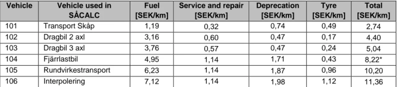
TABLE 6.1 DISTANCE BASE COST ELEMENTS FOR ROAD VEHICLES USED IN SAMGODS V1.1 ... 54

TABLE 6.2 DISTANCE BASED COST ELEMENTS FOR ROAD VEHICLES PRESENTED IN ASEK6.0 ... 54

TABLE 6.3 TIME BASED COST ELEMENTS FOR ROAD VEHICLES USED IN SAMGODS V1.1 ... 55

TABLE 6.4 TIME BASED COST ELEMENTS FOR ROAD VEHICLES USED IN ASEK6.0 ... 55

TABLE 6.5 TOLL CHARGE PER LORRY OUTSIDE SWEDEN USED IN SAMGODS V1.1 ... 56

TABLE 6.6 TOLL CHARGE PER LORRY OUTSIDE SWEDEN USED IN SAMGODS V1.1 ... 56

TABLE 6.7 DISTANCE BASED COST OF ELECTRICITY FOR RAIL VEHICLES ... 57

TABLE 6.8 TIME BASED COST ELEMENTS FOR RAIL USED IN SAMGODS V1.1[SEK/H] ... 57

TABLE 6.9 TIME BASED COST ELEMENTS FOR RAIL USED IN ASEK6.0[SEK/H] ... 58

TABLE 6.10 TRACK FEES FOR TRAINS USED IN SAMGODS V1.1[SEK/KM] ... 58

TABLE 6.11 TOLL FEES FOR TRAINS USED IN SAMGODS V1.1 ... 59

TABLE 6.12 DISTANCE BASED COST FOR VESSELS/FERRIES IN SAMGODS V1.1 AND ASEK6.0 ... 60

TABLE 6.13 TIME BASED COST FOR VESSELS USED IN SAMGODS V1.1 AND ASEK6.0 ... 61

TABLE 6.14 POSITIONING COSTS USED IN SAMGODS V1.1 ... 62

TABLE 6.15 FAIRWAY DUES IN SAMGODS V1.1 AND ASEK6.0 ... 63

TABLE 6.16 PASSAGE COSTS AT THE KIEL CANAL IN SAMGODS V1.1 ... 63

TABLE 6.17 LINK COSTS FOR AIR FREIGHT TRANSPORTS IN SAMGODS V1.1 ... 64

TABLE 6.18 LOADING AND UNLOADING COSTS CONVENTIONAL TRANSFER IN SAMGODS V1.1 ... 66

TABLE 6.19 LOADING WEIGHTS FOR ISO-CONTAINERS IN SAMGODS V1.1 AND ASEK6.0 ... 68

TABLE 6.20 LOADING/UNLOADING COSTS FOR CONTAINERS IN SAMGODS V1.1 AND ASEK6.0 ... 68

TABLE 7.1 OVERVIEW:OUTPUT FILES ... 71

TABLE 7.2 OVERVIEW OF COLUMNS IN THE FILE CHAINS<COMMODITY>.DAT ... 72

TABLE 7.3 OVERVIEW OF COLUMNS IN THE FILE CONNECTION.LST ... 72

TABLE 7.4 OVERVIEW OF COLUMNS IN THE FILE CHAINCHOI<COMMODITY>.FAC ... 73

TABLE 7.5 OVERVIEW OF COLUMNS IN THE FILE CHAINCHOI<COMMODITY>_<SOLUTION>.OUT ... 74

TABLE 7.6 OVERVIEW OF COLUMNS IN THE FILE CHAINCHOI<COMMODITY>_DATA_06.OUT ... 75

TABLE 7.7 OVERVIEW OF COLUMNS IN THE FILE CHAINCHOI<COMMODITY>_DATA_07.OUT ... 77

TABLE 7.8 OVERVIEW OF COLUMNS IN THE FILE CHAINCHOI<COMMODITY>.CST ... 78

TABLE 7.9 OVERVIEW OF COLUMNS IN THE FILE CHAINCHOI<COMMODITY>.REP ... 79

TABLE 7.10 OVERVIEW OF COLUMNS IN THE FILE LOCKED<COMMODITY>.LOG ... 80

(5)

5

TABLE 7.12 OVERVIEW OF COLUMNS IN THE FILE CONSOL<COMMODITY>_<MODE>.314 ... 80

TABLE 7.13 OVERVIEW OF COLUMNS IN FILE VOLUME_<COMMODITY>_<MODE>.314 ... 81

TABLE 7.14 OVERVIEW OF COLUMNS IN THE FILE OD_TONNES<VEHICLETYPE>.314 ... 81

TABLE 7.15 OVERVIEW OF COLUMNS IN THE FILE OD_VHCL<VEHICLETYPE>.314 ... 82

TABLE 7.16 OVERVIEW OF COLUMNS IN THE FILE OD_EMP<VEHICLETYPE>.314 ... 82

TABLE 7.17 OVERVIEW OF COLUMNS IN THE FILE STAN.DAT ... 83

TABLE 7.18 OVERVIEW OF COLUMNS IN THE FILE EMPTYCOST.DAT ... 83

TABLE 9.1 PREDEFINED TRANSPORT CHAINS ... 85

TABLE 9.2 VEHICLE TYPE IN BUILDCHAIN FOR EACH SUB-MODE BY COMMODITY TYPE ... 87

TABLE 9.3 TYPICAL SHIPMENT SIZES USED IN BUILDCHAIN. ... 89

TABLE 9.4 INVENTORY COSTS AND ORDER COSTS ... 90

TABLE 9.5 CURRENT AND SUGGESTED COST PARAMETERS FOR INLAND WATERWAY, VEH.322 ... 91

(6)

List of figures

FIGURE 3.1 ADMINISTRATIVE ZONES IN SWEDEN AND IN THE NEIGHBOURING COUNTRIES... 14

FIGURE 3.2 ADMINISTRATIVE ZONES IN EUROPE. ... 15

FIGURE 5.1 TERMINALS, PORTS AND NETWORKS ... 33

FIGURE 5.2 DOMESTIC ROAD NETWORK ... 36

FIGURE 5.3 RAIL NETWORK IN SWEDEN AND NEIGHBOURING COUNTRIES ... 39

FIGURE 5.4 SEA AND FERRY NETWORK INSIDE AND OUTSIDE SWEDEN, INCLUDING PORTS IN SWEDEN ... 42

(7)

7 Summary

The national model for freight transportation in Sweden is called Samgods. The purpose of the model is to provide a tool for forecasting and planning of the transport system. Samgods can be used in policy analysis such as studying the effects of a tax change or a change in transport regulation etc. The aim of this report is to give an overview of how the Swedish transport and logistics system is represented in the Samgods model. Samgods consists of several parts, where the logistics module is the core of the model system. This report describes the setup data (2016-04-01) needed to run version 1.1 of the Samgods model.

The 35 commodity groups used in the model are based on the 24 groups in the European NST/R- nomenclature. Some commodities are further divided due to their importance for Swedish freight transport and varying logistic properties. Transport demand is described with commodity specific demand matrices for 464 administrative zones inside and outside Sweden. Demand between sending zones (production, wholesale) and receiving zones (consumption) is described with the help of production-wholesale-consumption (PWC) matrices.

The commodity specific P, C or W zones are split into sub-cells that include firms. The method used to generate the firm to firm flows is to divide the firms at the origin zone and destination zone into three categories according to size. It is therefore a maximum of nine sub-cells per relation. A tenth cell is used for transit flows and single firms’ extremely large PC-flows. All small, medium and large firms are assumed to base their logistic decisions on the same

optimization principles. Only large firms are assumed to be able to have direct access to the rail and/or sea network.

A range of vehicle and vessel types are used to reflect scale advantages in transporting operations, including loading and unloading. The Samgods model uses six vehicle types for road, 10 for rail, 22 for sea and one for air. In total, 98 pre-defined transport chains are used. A distinction is made between container transports and non-container transports.

Infrastructure networks are used to generate the level of service (LOS)-matrix data for each vehicle/vessel type providing transport time and, distance and network related infrastructure charges. The LOS matrices supply information among all administrative PWC-zones and all terminals. There are a total of 171 LOS-matrices, consisting of 160 vehicle specific matrices (40 vehicle types * 4 cost/time matrices) and 11 frequency matrices used to determine wait time in terminals. CUBE-Voyager is used in order to produce the LOS-matrices.

The logistics costs consist of transport costs (vehicle type specific link costs and node costs) and non-transport costs (commodity specific order costs, storage costs and capital costs in inventory as well as capital costs in transit). For each commodity it is assumed that either the overall logistics costs are optimized or the transport costs are minimized. Combining smaller shipments into larger shipments are possible in order to maximize utilization of each transport, this

concept is known as consolidation. The current version of the model assumes that consolidation is only possible within a commodity group and can only be performed at terminals. In reality consolidation may also be possible on route in some extent, this is not taken into consideration in the model.

The model generates a huge amount of output at different levels. All the output files generated are described in the last chapter of this report.

(8)

1 Introduction

1.1 The Samgods model.

The national model for freight transportation in Sweden is called Samgods. The purpose of the model is to provide a tool for forecasting and planning of the transport system. Samgods can be used in policy analysis such as studying the effects of a tax change or a change in transport regulation etc. The model delivers transport solutions at the national level for import, export and transit flows. Samgods also handles domestic transport among municipilaties, and the ambition is to be able to model the regional level in the future. The Samgods model can also be used to extract cost data to be used in cost benefit analyses.

The Samgods model system consists of the following set of main software components:

 The logistics model, which is the core of the model system. In the logistics model, different types of commodities are assigned to different types of transport chains based on minimization of the total logistics cost. The logsitics model is documented in a method report [1] and a program documentation [2].

 The rail capacity model (RCM), which is a new feature to manage rail link flow volume constraints. The RCM model is documented in [3].

 Cube Base, where the graphical user interface (GUI) of Samgods is incorporated.

 Cube Voyager, which is a transport modelling software used to implement supply and assignment models.

 Cube GIS, which is the geographical information system where the network of the model is implemented.

In addition, there are two components that have been fully integrated in the model; ‘locked solution’ and ‘select link’. The component ‘locked solution’ gives the user a possibility to lock a logistics chain in a specific trade relation while the ‘select link’ component allows the user to trace all logistics chains that passes a selection of links.

A user manual for the Samgods model is provided in [4] and an overview of the file structure in the Samgods GUI is available in [5]. Further, the generation of transport demand matrices used in the model is documented in [6].

1.2 Developments of the Samgods model.

The aspect of logistics is crucial for understanding developments of the freight transport market, the modes of transport and infrastructure requirements. Therefore, it is important that the national freight model explicitly treats logistics choices. Example of such choices are the selection of shipment sizes, consolidation of shipments or the choice of road terminals. The Samgods model should, as realistically as possible, define the likely number of shipments per year, terminal passages, handling technologies used and routes of shipments.

As most freight transport models, the Swedish national freight model system were previously lacking treatment of logistics choices. Therefore, a process to update and improve the existing

(9)

9

national freight model system was started. An important part of this was the development of a logistics module. In 2005/2006, a prototype version of the logistics model using Swedish network and cost data, and data on the locations of terminals and distribution centers was developed. The purpose of this version was mainly to show the feasibility of the approach. After having shown that the approach was feasible, a new and extended version of the logistics model has been specified and applied for Sweden within the framework of their national freight transport forecasting system. Just recently, a version 2.1 of the logistics model has been documented in the form of a technical report [2].

The current version of the Samgods model is 1.1. Compared to the previous model version 1.0, Samgods 1.1 contains a range of updates, for example:

 New transport demand matrices. New method for calculation and updated base year from 2006 to 2012. Also, the forecast has been updated from 2030 to 2040.

 A new post processing model called Rail Capacity Management (RCM) has been added in order to handle limited track capacity.

 New transport costs, including an update to year 2014 prices.

 Five new vehicle types - three extra-long trains, an extra-heavy lorry and an inland waterway barge.

 A possibility to extract cost data to be used in cost benefit analyses.

 A possibility to lock a logistics chain for a specific trade relation.

 A possibility to trace all logistics chains that passes a selection of links.

1.3 Purpose and structure of the report

The purpose of this report is to give policy makers, researchers, consultants and users of the Samgods model an overview of how the Swedish transport and logistics system is represented in the Samgods model. The report includes a description of all input data necessary to run the Samgods model version 1.1 (setup dated 2016-04-01). The aim is to ensure that the transport system (infrastructure network including costs functions) is described and structured in a way that the clients’ requirements can be dealt with and facilitated.

The rest of the report is structured as follows;

- Chapter 2 describes the commodity classification used in the model.

- Chapter 3 describes the division of administrative zones, the PWC-matrices and generation of firm to firm flows, and firms’ access to infrastructure.

- Chapter 4 deals with the vehicle classification used in the model (modes, sub-modes and vehicle types) and the generation of transport chains.

- Chapter 5 describes the infrastructure networks and the generation of level of service (LOS) matrices.

(10)

- Chapter 6 describes the logistics costs used in the model and the optimization principles applied.

(11)

11 2 Commodity groups

2.1 Considerations regarding the commodity classification.

The commodity classification should reflect the real world. However, it is not possible to model all commodities, some aggregation is needed in order for the model to operate with acceptable run times. Also, the commodity classification needs to be designed in such a way that transport demand can be estimated with an acceptable statistical significance. The basis for aggregation should be homogeneity, i.e. the commodities in a commodity group should be similar with respect to logistic properties such as value and shipment size. Fewer commodity groups will give better run times, but on the other hand goods will be less homogenous. For the purpose of comparison, it is important that the classification is in line with nomenclatures used in official statistics. Also, it is important to note that the optimal number of commodity groups depends on the purpose of the analysis one wants to perform.

2.2 Commodity classification used in the model.

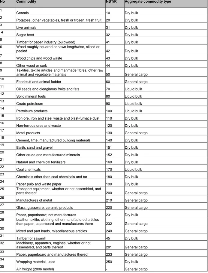
The Samgods model operates with 35 aggregated commodity groups (commodities). The division of commodities is based on the European commodity classification NST/R1_{which was}

standard in European statistics until 2007. In the NST/R-24 classification, commodities are represented by 24 commodity groups with subdivisions, making up a total of 30 commodity groups. For the purpose of the Samgods model, four commodities are further divided due to their varying logistic properties such as value and shipment size. For example, the group Paper and pulp is split into Paper pulp and waste paper (Commodity 24) and Paper, paperboard and manufactures thereof (Commodity 33). Further, a commodity group for goods transported by air freight (Commodity 35) is created by allocating fractions of certain commodities to group 35. The reason for this approach is that not even small shares of the commodities would go by air solely based on their logistics costs.

Commodities 8, 30 and 34 are not used in the Samgods model version 1.1. This is because the data necessary for the construction of transport demand matrices are unavailable for these commodity groups.

All commodities are associated with an aggregate commodity type: dry bulk, liquid bulk or general cargo (which in turn defines e.g. which costs apply, see section 6.4) The value of each commodity, expressed in SEK/tonne in year 2012 prices, were derived in the base matrix project [6]. In contrast to previous model versions, Samgods 1.1 uses separate values for domestic transports, transit, import and export. Table 2.1 presents the 35 commodity groups along with the NST/R code and aggregate commodity type.

(12)

Table 2.1 Commodity classification and aggregate commodity type.

No Commodity NST/R Aggregate commodity type

1

Cereals 10 Dry bulk

2

Potatoes, other vegetables, fresh or frozen, fresh fruit 20 Dry bulk 3

Live animals 31 Dry bulk

4

Sugar beet 32 Dry bulk

5

Timber for paper industry (pulpwood) 41 Dry bulk

6 Wood roughly squared or sawn lengthwise, sliced or

peeled 42 Dry bulk

7

Wood chips and wood waste 43 Dry bulk

8

Other wood or cork 44 Dry bulk

9 Textiles, textile articles and manmade fibres, other raw

animal and vegetable materials 50 General cargo

10

Foodstuff and animal fodder 60 General cargo

11

Oil seeds and oleaginous fruits and fats 70 Liquid bulk 12

Solid mineral fuels 80 Liquid bulk

13

Crude petroleum 90 Liquid bulk

14

Petroleum products 100 Liquid bulk

15

Iron ore, iron and steel waste and blast-furnace dust 110 Dry bulk 16

Non-ferrous ores and waste 120 Dry bulk

17

Metal products 130 General cargo

18

Cement, lime, manufactured building materials 140 Dry bulk 19

Earth, sand and gravel 151 Dry bulk

20

Other crude and manufactured minerals 152 Dry bulk 21

Natural and chemical fertilizers 160 Dry bulk

22

Coal chemicals 170 Liquid bulk

23

Chemicals other than coal chemicals and tar 180 Dry bulk 24

Paper pulp and waste paper 190 Dry bulk

25 Transport equipment, whether or not assembled, and

parts thereof 200 General cargo

26

Manufactures of metal 210 General cargo

27

Glass, glassware, ceramic products 220 General cargo

28

Paper, paperboard; not manufactures 231 Dry bulk

29 Leather textile, clothing, other manufactured articles

than paper, paperboard and manufactures there 232 General cargo 30

Mixed and part loads, miscellaneous articles 240 General cargo 31

Timber for sawmill 45 Dry bulk

32 Machinery, apparatus, engines, whether or not

assembled, and parts thereof 201 General cargo

33

Paper, paperboard and manufactures thereof 233 General cargo 34

Wrapping material, used 250 Dry bulk

35

(13)

13 3 Zones, firms and their access to

infrastructure

The purpose of the Samgods model is to provide a tool for planning and forecasting of the transport system. In order to do this, the model needs input data on trade (goods flows) among firms. In Samgods, this is solved by using the following steps. First, transport demand (PWC matrices) are estimated for 464 administrative zones (geographic regions) using data from the Swedish commodity flow survey. Second, transport demand are decomposed to the firm to firm level by dividing firms into three categories according to size. The logistic decision is then simulated at the firm to firm level. In this chapter we describe the zoning system, the estimation of transport demand and the decomposition to the firm to firm level, and assumptions regarding the firms’ access to infrastructure.

3.1 Administrative zones

There are a total of 464 regional administrative zones in the Samgods model, of which 290 are domestic municipalities and 174 are foreign zones.

3.1.1 Domestic zones

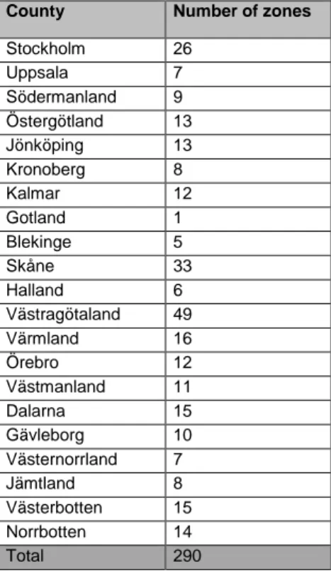
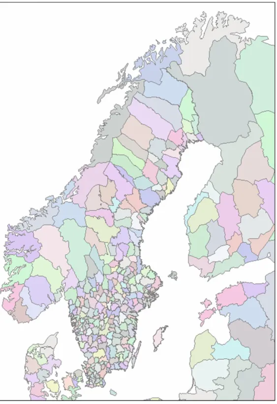
The 290 domestic zones corresponds to the 290 municipalities of Sweden. The domestic zone numbers are based on the official municipality numbers used by Statistics Sweden. All domestic administrative zones finish with 00 and are in the range 711400-958400. Table 3.1 below shows the number of zones per county in Sweden. The zones in Sweden and in the neighbouring countries are visualized in figure 3.1.

Table 3.1 Number of administrative zones per county in Sweden

County Number of zones

Stockholm 26 Uppsala 7 Södermanland 9 Östergötland 13 Jönköping 13 Kronoberg 8 Kalmar 12 Gotland 1 Blekinge 5 Skåne 33 Halland 6 Västragötaland 49 Värmland 16 Örebro 12 Västmanland 11 Dalarna 15 Gävleborg 10 Västernorrland 7 Jämtland 8 Västerbotten 15 Norrbotten 14 Total 290

(14)

(15)

15 3.1.2 International zones

Inside Europe

There are a total of 174 zones outside Sweden of which 149 are located inside Europe. Of these 149 zones, 68 are located in the neighbouring countries (Norway, Finland, Denmark and Germany). Within Europe, the further away from Sweden, the fewer zones per country. When sorted numerically, the foreign zones come after the domestic zones. The foreign zones inside Europe also finish with 00 and are in the range 960100-974900.

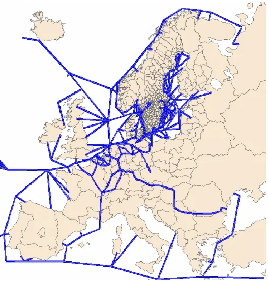
The administrative zones within Europe are visualized in figure 3.2.

Figure 3.2 Administrative zones in Europe.

Outside Europe

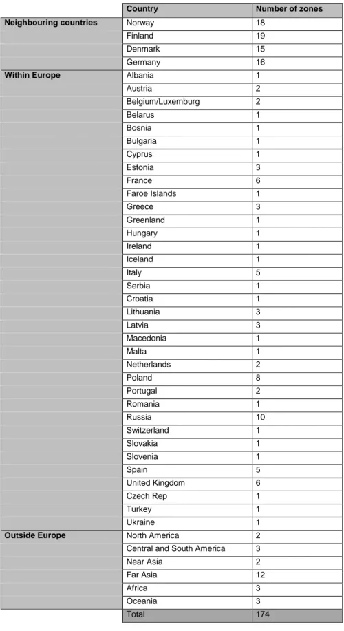
There are a total of 25 administrative zones outside Europe. Countries that are significant trading partners to Sweden are defined as unique zones while other countries with smaller trading flows is aggregated into one joint zone for each continent. Zone numbers above 97500 indicates a location outside Europe.

(16)

Table 3.2 Number of zones per country/region outside Sweden.

Country Number of zones

Neighbouring countries Norway 18

Finland 19

Denmark 15

Germany 16

Within Europe Albania 1

Austria 2 Belgium/Luxemburg 2 Belarus 1 Bosnia 1 Bulgaria 1 Cyprus 1 Estonia 3 France 6 Faroe Islands 1 Greece 3 Greenland 1 Hungary 1 Ireland 1 Iceland 1 Italy 5 Serbia 1 Croatia 1 Lithuania 3 Latvia 3 Macedonia 1 Malta 1 Netherlands 2 Poland 8 Portugal 2 Romania 1 Russia 10 Switzerland 1 Slovakia 1 Slovenia 1 Spain 5 United Kingdom 6 Czech Rep 1 Turkey 1 Ukraine 1

Outside Europe North America 2

Central and South America 3

Near Asia 2

Far Asia 12

Africa 3

Oceania 3

(17)

17 3.2 PWC-matrices and disaggregation to firms

Estimation of PWC matrices

In Samgods, the transport demand between sending zones (production) and receiving zones (consumption) is described with the help of production-wholesale-consumption (PWC) matrices. Wholesale (W) is treated separately because of the fact that wholesalers’ logistic requirements differ from producers’ requirements. The PWC matrices describe the demand for goods transport from one place to another, so that the matrix element (r, s) gives the amount of goods to be transported from zone r to zone s.

The base matrices for the year 2012 derived in the base matrix project are used in Samgods version 1.1 [6]. In total, there are 32 commodity specific demand matrices for

464 administrative zones. The estimation of PWC matrices is based on data from the Swedish commodity flow survey (CFS) for the years 2001 and 2004/05. Since the CFS data are collected using a sample survey, some uncertainty is inevitable. It is important to note that this

uncertainty is inherited into the PWC matrices. Moreover, due to data insufficiency, no PWC matrices were possible to estimate for commodities 8, 30 and 34. Further, the information extracted from the CFS are not sufficient to distinguish wholesale (W) and consumption (C) at the receiver side. Thus, special treatment of wholesale (W) is possible only at the sender side. Another problem is that the number of CFS-observations on foreign trade is rather small. Given these data inadequacies, it is important to acknowledge that there might be a gap between the estimated PWC matrices and the true transport demand.2

Decomposing transport demand to the firm to firm level

The Samgods model runs at a virtual firm level. Therefore, the commodity specific P, C or W zones are split into sub-cells that include firms. The method used to generate the firm to firm flows is to divide the firms at the origin zone and destination zone into three categories according to size (number of employees). The three categories are:

 small firms (first 33 % of the firm size distribution)

 medium firms (34-66% of the firm size distribution)

 large firms (67-100% of the firm size distribution)

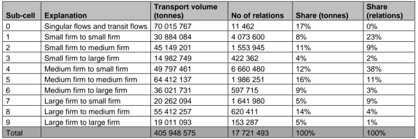
Combining sending and receiving firms, we have 9 possible sub-cells per relation (see table 3.3 below). Further, a tenth sub-cell (No 0) is used for so called singular flows and transit flows. Singular flows are single firms’ extremely large PC-flows. Transit flows start and end outside Sweden and are transported ashore on Swedish territory.

Table 3.3 summarizes the 10 sub-cells used in the PWC matrices. Further, it gives information about the distribution of transport volume and the number of relations per sub-cell. For

example, even though singular flows and transit flows only amounts to about 11 thousand out of 18 million relations, this sub-cell is responsible for 17 % of the total transport volume.

2_{For further details regarding data and estimation of PWC matrices, see Varuflödesundersökningen}

2004/2005 (SIKA, 2006) and PWC Matrices: new method and updated Base Matrices (Anderstig et al, 2015).

(18)

Table 3.3 Distribution of transport volume and relations per sub cell.

Sub-cell Explanation

Transport volume

(tonnes) No of relations Share (tonnes)

Share (relations)

0 Singular flows and transit flows 70 015 767 11 462 17% 0%

1 Small firm to small firm 30 884 084 4 073 600 8% 23%

2 Small firm to medium firm 45 149 201 1 553 945 11% 9%

3 Small firm to large firm 14 982 749 422 362 4% 2%

4 Medium firm to small firm 49 797 461 6 660 480 12% 38%

5 Medium firm to medium firm 64 412 137 1 986 251 16% 11%

6 Medium firm to large firm 36 021 731 597 715 9% 3%

7 Large firm to small firm 20 262 094 1 641 980 5% 9%

8 Large firm to medium firm 55 412 257 620 411 14% 4%

9 Large firm to large firm 19 011 093 153 287 5% 1%

Total 405 948 575 17 721 493 100% 100%

All small, medium and large firms are assumed to base their logistic decisions on the same optimization principle (see 6.4). However, logistic decisions such as the choice of transport chains differ due to the firm’s annual transport volume and number of firm to firm relations. Also, the access to infrastructure differ by the size of the firm (more on this in section 3.3.).

3.3 Firms’ access to infrastructure

3.3.1 Inside Europe

Road

In the Samgods model, it is assumed that all sending and receiving firms have direct access to the road network and via this network to other modes such as rail, sea and air. This means that goods flows from/to firms located at the centroid (the business centre of a zone) will start/end with a road link.

Rail and sea

In some cases, industrial producers and/or consumers have, via industrial tracks , direct access to the rail network or are located in ports. One example is the iron-ore produced in the mines of Kiruna. Similarly, crude oil is transferred directly from vessels to oil terminals within ports - not first unloaded and then re-loaded for further transport to the business centre. In the Samgods model, direct access to the rail and/or sea network is assumed to be available only when a large firm is involved.3_{Thus, direct access is assumed to be available for sub-cells 3,6,7,8, and 9. This}

assumption is clearly a simplification of reality. For the sea mode for example, there are probably small firms located in ports that use sea transport as first/last link.

However, not all large firms are assumed to have direct access to the rail and/or sea network. If the large firm is assumed to have direct access or not depends on the location of the firm and the commodities produced. For feeder and wagonload trains, direct access is available for all

commodities but not all zones. Feeder and wagonload trains are used together in a transport chain, feeder trains act as a “feeder” for the wagonload train i.e. are used as the first or last link. However, feeder trains are only specified within Sweden. The reason for this simplification is that the primary interest of the model is the Swedish transport system, and it is therefore

(19)

19

appropriate to be more detailed at the national level. Further, the knowledge about foreign transport systems is limited. Direct access for feeder trains are thus present only in Sweden while direct access for wagonload trains are present only for zones outside Sweden (in Europe). Direct access to system trains and sea is specified per zone and commodity. The reason for this is that certain locations and/or commodities are more suited for these type of transports, e.g. the iron-ore produced in Kiruna mentioned above. In Sweden, direct access to system trains is available at 63 locations. Other than Narvik (part of the iron ore corridor) and Torneå (connects the Swedish railroad network to Finland and Russia), no direct access for system trains exist outside Sweden. For sea, direct access is available in 41 domestic zones while direct access outside Sweden is limited to the port of Narvik. Again, the reason behind these simplifications is the need to be detailed at the national level and the availability of adequate information.Table 3.4 summarizes the information on direct access to rail and sea in Sweden and the rest of Europe.

Table 3.4 Direct access to rail and sea.

Commodity specific Number of

locations in Sweden Number of locations in Europe outside Sweden Total number of locations in Europe Direct access to feeder trains No 152 0 152 Direct access to wagonload trains No 0 28 28 Direct access to system trains Yes 63 2 65

Direct access to sea Yes 41 1 42

Air

The Samgods model does not include any direct access for air transport in Europe. This is because airports are not assumed to be the start or end location of any goods flow (at the PWC level). It is necessary to first transport the goods by lorry to and from the airport.

3.3.2 Outside Europe

The Samgods model does not explicitly model land-based networks outside Europe, but it is assumed that all transports start or end in a port or airport that, via a virtual link, is connected to the zone centroid without any distance or cost. Direct access to sea and air is assumed for all zones outside Europe. One difference between sea and air is that direct access to sea has to be specified in the input files while direct access to air is always assumed for airborne flows outside Europe.

These assumptions are clearly a non-realistic simplification of reality, but are necessary to ensure that these zones are connected to Sweden. Again, the model is limited by the information available about foreign transport systems. However, it can be argued that land-based transport cost for shipments that starts or end outside Europe is a relatively small part of the total logistics cost and the results would thus not be affected in any significant way. Further, as stated earlier in this chapter, the primary interest of the Samgods model is to analyse effects in the Swedish transport system. Thus, the conclusion is to have a model that are less detailed the further away from Sweden we get.

(20)

4 Vehicles/vessels, cargo units and transport

chains

In order for the Samgods model to be able to simulate logistic decisions, it is necessary to specify available vehicles and in which combinations (i.e. transport chain) they can be used. In

Samgods, this is solved by introducing vehicle types and sub-modes, and by defining pre-set transport chains. This is what will be described in this chapter. Note that throughout the chapter the term “vehicle” will be used to address both vehicles and vessels. The term “mode” refer to the aggregate transport modes; road, rail, sea and air.

4.1 Vehicle classification

4.1.1 Considerations regarding the vehicle classification.

The vehicle classification should reflect the real world. However, it is not possible to model all vehicles, some selection is needed in order for the model to operate efficiently. There are several aspects to consider when it comes to the vehicle classification. It is important to consider economies of scale, the nature of the goods to be transported, wear and tear of infrastructure, laws and regulations and, of course, vehicle classification used in other transport related models. These issues are discussed below.

Economies of scale at the vehicle level

For each mode of transport, several vehicle types are used in the model in order to reflect scale advantages in transporting operations, including loading and unloading. Per provided capacity unit, using larger vehicles leads to lower costs. Given a good capacity utilisation for the vehicles employed, there are scale economies in vehicle size for all modes. For rail, economies of scale are possible to model only at the train level. In reality however, scale advantages exist at both the train and the wagon level.

Goods to be transported

Some of the products require special handling equipment for loading and unloading and/or specific vehicles. For example, liquid matters require tanks and pumps. Because of these

product related differences, it might seem natural to differentiate vehicle type also by product. A combined classification could thus be vehicle size and type of commodity to be transported. However, such product related additions to the vehicle classification should only be made if the differences have a significant influence on the costs for any given vehicle size, or if the relevant range as well as class of vehicle sizes differ significantly for different products. The commodity based approach chosen in the Samgods model uses few vehicle types and focuses on scale advantages. Following this approach, the best solution is to have as few product related exceptions as possible.

Infrastructure requirements, law and regulations

The state of infrastructure as well as law and regulations put restrictions on the vehicles that can be used in the transport system. They are, of course, closely linked to each other. For example, infrastructure/regulations is a limiting factor for road transport since the highest carrying capacity/maximum permissible weight on roads are currently 64 tonnes. Also, different vehicle types influence wear and tear of infrastructure differently. This implies that the size of the vehicles should be expressed in dimensions that are relevant to the infrastructure holders.

(21)

21

The Samgods vehicle classification in relation to other transport models.

It is important to consider how the vehicle classification compares to other transport related models. First, the vehicle classification should follow the guidelines set out in the ASEK report (Analysmetod och samhällsekonomiska kalkylvärden för transportsektorn), which is a

compilation of model parameters recommended to be used in all transport analyses performed by Trafikverket [7]. However, there are some discrepancies between the vehicle types included in the current ASEK 6.0 and the vehicle classification used in Samgods:

- Road: The 74 tonnes lorry (vehicle type 106) defined in Samgods is not present in ASEK. This lorry type is currently not permitted on Swedish roads, but the government has plans to allow for high capacity transport in the near future. This is the reason why it is included in Samgods (see section 4.1.3).

- Rail: The extra-long wagonload train (vehicle type 212) defined in Samgods is not included in ASEK. However, ASEK includes an extra-long system train with a maximum permissible axle load weight of 25 tonnes that is not present in Samgods. - Sea: no differences in classification (however, there are differences in the costs applied,

see chapter 6)

- Air: ASEK does not include any information regarding air transport.

It is also important to consider that the Samgods forecast is used as input in other transport models. The forecast generated in Samgods is used as input in EVA, Sampers/Samkalk, Bansek and TEN-Tec

- EVA is a tool used to analyse and calculate effects for road traffic. The Samgods forecast provides the relevant information needed to generate growth in vehicle kilometres for lorries used as input in EVA. The EVA model does not distinguish between different lorry types.

- Bansek is a tool used to produce CBA output for railroad projects. The Samgods forecast provides the relevant information needed to generate growth in vehicle kilometres used as input in Bansek. The model includes the following train types; long-distance

wagonload train, local wagonload train, system train, kombi-train and trains transporting ore.

- Sampers/Samkalk is a national model system used in transport analyses for passenger transport. Sampers/Samkalk does not model goods transport explicitly. However, road and rail congestion is affected not only by passenger transport, but also the number of goods transports in the system. Therefore, the goods flows simulated in Samgods are added to the road and rail networks used in Sampers/Samkalk.

TEN-Tec is the European Commission’s Information System used to coordinate and support the

Trans-European Transport Network Policy (TEN-T). The Samgods forecast is used to provide

information about the goods flows at the 25 Swedish ports included in the TEN-T.

(22)

4.1.2 Vehicle types used in the model

Given the considerations above, 40 vehicle types are defined in the Samgods model. The 40 vehicle types cover:

- 6 road vehicles (no 101 – 106),

- 11 train types (no 201 – 212, no 203 is not defined), - 22 sea vessels (no 301 – 322)

- 1 freight airplane (no 401)

Compared to Samgods 1.0, version 1.1 has 5 new vehicle types; one extra heavy lorry is added to the road mode, 3 extra-long trains are added to the rail mode and one inland waterway barge is added to the sea mode (the reason for adding new vehicle types are discussed below under the headline for respective mode).

Table 4.1 includes information about the vehicle types and the weight capacity of each vehicle. When it comes to rail, trains are used as vehicle units, not single wagons. The capacities have to be seen as maximum values. It is important to note that for many bulky products, it is the volume that is the limiting factor – not the weight.

(23)

23

Table 4.1 Vehicle classification

Mode Vehicle

number

Vehicle name Capacity

(tonnes per vehicle)

Road 101 _{Lorry light LGV.< 3.5 ton} ₂

102 _{Lorry medium 3.5-16 ton} ₉

103 _{Lorry medium16-24 ton} ₁₅

104 _{Lorry HGV 25-40 ton} ₂₈

105 _{Lorry HGV 25-60 ton} ₄₇

106 _{Lorry HGV 74 ton} ₆₂

Rail 201 _{Kombi train} ₆₁₀

202 _{Feeder/shunt train} ₄₈₈

204 _{System train STAX 22.5} ₉₅₉

205 _{System train STAX 25} ₁₀₉₈

206 _{System train STAX 30} ₆₀₀₀

207 _{Wagon load train (short)} ₇₁₆

208 _{Wagon load train (medium)} ₈₅₂

209 _{Wagonload train (long)} ₉₀₇

210 _{Combi train (XL 750 m 201L)} ₉₈₀

211 _{System train STAX 22,5 (XL 750 m 204L)} ₁₄₀₀

212 _{Wagonload train (XL 750 m)} ₁₄₈₀

Sea 301 _{Container vessel 5.300 dwt (ship)} ₅₃₀₀

302 _{Container vessel 16.000 dwt (ship)} ₁₆₀₀₀

303 _{Container vessel 27.200 dwt(ship)} ₂₇₂₀₀

304 _{Container vessel 100.000 dwt (ship)} ₁₀₀₀₀₀

305 _{Other vessel 1.000 dwt (ship)} ₁₀₀₀

306 _{Other vessel 2.500 dwt (ship)} ₂₅₀₀

307 _{Other vessel 3.500 dwt (ship)} ₃₅₀₀

308 _{Other vessel 5.000 dwt (ship)} ₅₀₀₀

309 _{Other vessel 10.000 dwt (ship)} ₁₀₀₀₀

310 _{Other vessel 20.000 dwt (ship)} ₂₀₀₀₀

311 _{Other vessel 40.000 dwt (ship)} ₄₀₀₀₀

312 _{Other vessel 80.000 dwt (ship)} ₈₀₀₀₀

313 _{Other vessel 100.000 dwt (ship)} ₁₀₀₀₀₀

314 _{Other vessel 250.000 dwt (ship)} ₂₅₀₀₀₀

315 _{Ro/ro vessel 3.600 dwt (ship)} ₃₆₀₀

316 _{Ro/ro vessel 6.300 dwt (ship)} ₆₃₀₀

317 _{Ro/ro vessel 10.000 dwt (ship)} ₁₀₀₀₀

318 _{Road ferry 2.500 dwt} ₂₅₀₀

319 _{Road ferry 5.000 dwt} ₃₀₀₀

320 _{Road ferry 7.500 dwt} ₄₅₀₀

321 _{Rail ferry 5.000 dwt} ₅₀₀₀

322 _{Barge Inland water way} ₂₀₀₀

(24)

4.1.3 Road

Six typical road vehicles represent lorries (with or without trailer) of various sizes:

- One light lorry under 3.5 tonnes of total weight (total weight includes lorry and goods). - Two medium sized lorries with 16 tonnes resp. 24 tonnes of total weight.

- Three heavy duty lorries with 40, 60 and 74 tonnes of total weight.

The defined lorry types are chosen based on infrastructure constraints, regulations, lorry types used in other EU-countries and the need to model economies of scale. In Sweden, a ”light lorry” is a lorry with a total weight under 3.5 tonnes that can be driven by anyone with a driver’s license while a ”heavy lorry” is a lorry with a total weight over 3.5 tonnes that requires a special license. The 40 tonnes lorry is standard in most EU-countries whereas the 60 tonnes lorry is common in Sweden and Finland. The 74 tonnes lorry is currently not allowed on Swedish roads. However, the Swedish government have plans to allow for high capacity transport (HCT) on roads in the future.4

4.1.4 Rail

In the Samgods model, a total of eleven train types are defined (but only ten types are used). The use of different vehicle types is driven by the existence of different production systems for rail transport (and the need to model economies of scale):

- Combined trains (combi trains) require unitised cargo units like containers (see section 4.2). These trains combine road and sea with rail. There are two types of combi trains in the model, one regular and one long (750 m).

- There are five wagonload trains defined in the model, but only 4 are used. The first type acts as a feeder or shunt train between industrial locations and marshalling yards while the other four types, with differing lengths, act as long-distance trains between

marshalling yards. The wagonload system is used for goods with different destinations and fixed frequencies between marshalling yards. Note that vehicle type 209, wagonload train (long), is currently not used in the model. Instead, an extra-long wagonload train (750 m) has been added.

- There are four types of system trains. These trains are block trains, normally for a single commodity that go with a fixed frequency from one industrial location to another. There are three sizes of system trains depending on the maximum permissible axle weight (STAX). These are ≤ 22.5 tonnes, ≤ 25 tonnes and ≤ 30 tonnes per axle. The system trains with 25 and 30 tonnes maximum axle load are available for a limited part of the rail network and only for certain products. The forth type is a longer version (750m) of the 22.5 STAX train.

The Samgods model 1.1 has three new train types compared to the previous model version. One extra-long train (750 m) has been added to each train type. Such long trains can currently be

4_{On May 13 2015, Trafikverket recieved a request from the Swedish government to investigate and in}

depth analyze the effect of allowing HCT transport on Swedish roads. For further details, see the report Systemanalys av införande av HCT på väg, Trafikverket (2015).

(25)

25

used only at some parts of the Swedish railroad network. The reason is that most parts are not built to handle such long trains. For example, the meeting/passing stations are often not sufficiently long. However, the possibility to use longer trains for goods transport in Sweden is planned to be extended in the future.5

For rail, economies of scale are possible to model at the train level. In Samgods version 1.1 this possibility has been extended by the addition of the extra-long (750 m) trains. Since trains are used as the vehicle unit, it is not possible to model economies of scale at the wagon level in the current model. This has complications for an analyst who wants model train flows at a more detailed level.

Different types of freight trains display certain speed differences. However, speed differ more according to infrastructure characteristics than to train types and the train speeds are therefore coded universally for all train types per link in the network.

4.1.5 Sea

The 22 vehicle types for the sea mode includes:

- four container vessels, cargo ships used to carry intermodal containers.

- three ro/ro vessels, ”roll on/roll off” ships designed to carry wheeled cargo transported in e.g. cars, trucks and railroad cars.

- ten “other vessels”, including all non-container and non-roro vessels that carry different commodities i.e. dry bulk vessels, dry cargo ships and tankers.

- three road ferries - one rail ferry

- one inland water way barge used for inland waterway transport.

For vessels, the economies of scale aspect is taken care of by defining the vessel’s capacity in dead-weight (dwt), i.e. the approximate cargo carrying capacity in weight terms in tonnes. Vessels with similar dwt-capacity tend to have similar draught, although there are differences in draught for the same dwt between various vessel categories (tankers, bulk carriers, container vessels etc.) due to different “lines” in the ship design. Sea vessels, as opposed to most land-based vehicles, differ significantly in size and therefore cost. The sea vessels, as defined in the Samgods model, vary from as little as 1 000 tonnes dwt to a maximum of 250 000 tonnes dwt. In the model, a total of 17 different vessels are defined (it is taken into account that certain products/commodities due to their density are transported in vehicles that require more depth than average vessels).

Ferries are in a way part of the road or rail network since they could be replaced by bridges or tunnels. Ferry capacity is normally shared by different firms and commodities. Economies of scale are less relevant for ferries than for vessels; when the size increases the decrease in unit

5_{On April 16 2015, Trafikverket received a request from the Swedish government to investigate the}

possibility to use longer trains in the existing Swedish railroad network. For further details see the report Regeringsuppdrag – Möjligheter att köra längre och/eller tyngre godståg, Trafikverket (2015).

(26)

costs is larger for vessels than for ferries. In the model, three road ferries (but only the smallest road ferry is used) and one rail ferry are defined.

Samgods 1.1 contains one new vehicle type for the sea mode compared to the previous model version. An inland water way barge (INW) has been added. Sweden has previously chosen not to implement the EU regulations for inland waterway transport. However, since the Swedish shipping industry has shown an increasing interest in this particular type of transport, Sweden has chosen to implement the same regulations as in continental Europe. Thus, since the 16th of December 2014 it is possible to build or equip ships for inland waterway transport also in Sweden.6

There are speed differences between certain types of vessels. Notable examples are between container vessels (20-30 km/h), ro-ro vessels (19-24 km/h) and other vessels (11-22 km/h).

4.1.6 Air

In the Samgods model, one cargo-specific aircraft (freighter) with a maximum capacity of 50 tonnes is defined. This means that freight transports in passenger air planes, so called pax belly transports, are not included.

4.2 Cargo units

Inter modal transports use unitised cargo types and at least two modes of transport. These transports are interesting as they combine the comparative advantages of the different modes. From an analysis perspective it is also important to know the potential for inter modal

transports. Conventional freight models use commodity and vehicle classifications but it is much less common to categorize cargo types. There is not much experience when it comes to the modelling of cargo units.7

In the Samgods model, the modelling of unitised transports is limited to container transports, in contrast to conventional load on/load off transports. Further, it is assumed that containers can be transported on nearly all vehicle and vessel types. Exceptions are the light and medium sized lorries, system trains and airplanes. On the other hand, kombi trains and container vessels are assumed to be used for container transports only. It is also assumed that the container is carried the entire transport chain from the sender to the receiver. Thus, it is not possible to stuff or strip a container along the transport. However, such stuffing and stripping can of course occur in reality, for example in ports.

6_{For further details, see information available at the Swedish Transport Agency’s website,}

https://www.transportstyrelsen.se/sv/Sjofart/Fartyg/Inlandssjofart/

7_{The use of international sea containers has been modelled in the 2005 version of the STAN-model. See}

(27)

27 4.3 Sub-modes and transport chains.

The Samgods model operates with predefined transport chains and each chain can contain a maximum of five legs. If the vehicle classification would be used for this purpose there would be a great number of possible chains and the run time of the model would not be adequate.

Therefore, in order to reduce the number of transport chains, sub-modes are created as a link between the mode and the vehicle type. There are a total of 19 sub-modes in the model:

- Three road modes: light lorry, heavy lorry and extra heavy lorry.

- Nine rail modes: one feeder train, two type of wagonload trains (regular and long), two type of combi-trains (regular and long) and four different system trains with maximum axle loads (STAX) of 22,5 ton, 25 ton and 30 ton including one regular and one long for the STAX 22,5 train.

- Six sea modes: direct sea, feeder vessel, long haul vessel, inland waterway barge, road ferry and rail ferry.

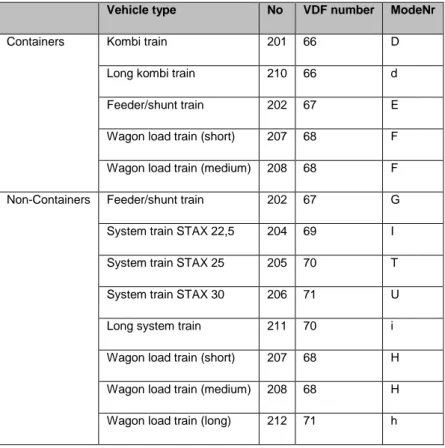
The sub-modes are given separately for container transports and non-container transports. The modes, sub-modes and vehicle types assumed in the model is shown in table 4.2.

When it comes to sea transports, a distinction between direct sea and feeder/long haul transports is made. Direct sea transports include only one sea link while feeder and long haul transports build sea-sea links. It is assumed that small feeder vessels “feed” large long haul vessels that go overseas. Thus, feeder ships and long-haul vessels must appear together in a transport chain. Ferry links are handled as sea legs within road or rail chains i.e. they can only appear as an intermediate leg in a transport chain.

As stated above in section 4.1.4, feeder trains act as a “feeder” for the wagonload train.

Therefore, feeder and wagonload trains must appear together in a transport chain (feeder train- wagonload train or vice versa). However, since feeder trains are only specified in Sweden (see section 3.3.1), this is not true for transports in the rest of Europe.

In Samgods 1.1, there are a total of 98 pre-defined transport chains. The available transport chains can be found in table 9.1 in the appendix. The pre-defined transport chains can be changed via the input files.

A sub-program of the logistics model, Buildchain, is then used to specify the transfer points per chain using one specified vehicle/vessel type for each leg and commodity. In order to do this, a typical vehicle is defined for each sub-mode and commodity. The typical vehicle is shown in table 9.2 in the appendix. Further, the BuildChain program also requires pre-set typical

shipment sizes as input parameters. The average shipment size per commodity is shown in table 9.3 in the appendix. The following step, Chainchoi, (another sub-program of the logistics model) optimises by choosing the best vehicle per mode category for each leg. For further details, see the program documentation of the logistics model [2].

(28)

Table 4.2 Modes, sub-modes and vehicle types.

Mode Sub-mode Sub-ModeNr VhclNr Vehicle type Container transport

Road Heavy lorry A 104 Lorry HGV 25-40 ton Yes

105 Lorry HGV 25-60 ton

Extra heavy lorry X 106 Lorry HGV 74 ton

Rail Kombi train D 201 Kombi train

Long kombi train d 210 Combi train (XL 750 m 201L)

Feeder train E 202 Feeder/shunt train

Wagonload train F 207 Wagon load train (short)

208 Wagon load train (medium)

Long wagonload train f 212 Wagon load train (long)

Sea Direct sea J 301 Container vessel 5.300 dwt (ship)

302 Container vessel 16.000 dwt (ship)

303 Container vessel 27.200 dwt(ship)

305 Other vessel 1.000 dwt (ship)

315 Ro/ro vessel 3.600 dwt (ship)

Feeder vessel K 301 Container vessel 5.300 dwt (ship)

Long-haul vessel L 303 Container vessel 27.200 dwt(ship)

INW V 322 Barge Inland water way

Road Light Lorry B 101 Lorry light LGV.< 3.5 ton No

102 Lorry medium 3.5-16 ton

103 Lorry medium16-24 ton

Heavy lorry C,S8 ₁₀₄ _{Lorry HGV 25-40 ton}

105 Lorry HGV 25-60 ton

Extra heavy lorry c 106 Lorry HGV 74 ton

8_{Consolidated heavy lorry is coded as mode S in the chains file. Consolidation in heavy lorries is only}

(29)

29

Mode Sub-mode Sub-odeNr VhclNr Vehicle type Container transport

Rail Feeder train G 202 Feeder/shunt train No

Wagonload train H 207 Wagon load train (short)

208 Wagon load train (medium)

Long wagonload train h 212 Wagon load train (long)

System train STAX 22,5 I 204 System train STAX 22.5

System train STAX 25 T 205 System train STAX 25

System train STAX 30 U 206 System train STAX 30

Long system train i 211

System train STAX 22,5 (XL 750 m

204L)

Sea Direct sea M 305 Other vessel 1.000 dwt (ship)

Feeder vessel N 315 Ro/ro vessel 3.600 dwt (ship)

Long-haul vessel O 317 Ro/ro vessel 10.000 dwt (ship)

INW W 322 Ro/ro vessel 6.300 dwt (ship)

Road ferry P 318 Road ferry 2.500 dwt

319 Road ferry 5.000 dwt

320 Road ferry 7.500 dwt

Rail ferry Q 321 Rail ferry 5.000 dwt

(30)

5 Networks and LOS-matrices

The following chapter gives an overview of the level of service-matrices, the links and the nodes for respective transport mode.

5.1 Background

The infrastructure networks are used for several purposes. One is to generate the level of service (LOS)-matrix data for each vehicle type.CUBE-Voyager is used in order to produce the LOS-matrices. The LOS-matrices are providing the vehicle transport time, distance and network related infrastructure costs for the route that has the lowest generalized cost (= Time*(vehicle cost/hour) + Distance*(vehicle cost/km) + road taxes/bridge tolls/rail fees) per vehicle type for all allowed OD-relations [3]. The LOS matrices supply information between all zones

(administrative PWC-zones and terminal zones). In some cases a service frequency per week is used for the OD-relations (for instance 84 trips per week for the ferry Helsingborg-Helsingör). Vehicle type specific LOS-matrices have been extracted:

Total distance matrix (km) dist

Domestic-only distance matrices (km) ddist

Pure time matrix (h) time

Infrastructure charges/fees matrix (kr) xkr

Frequency matrices freq

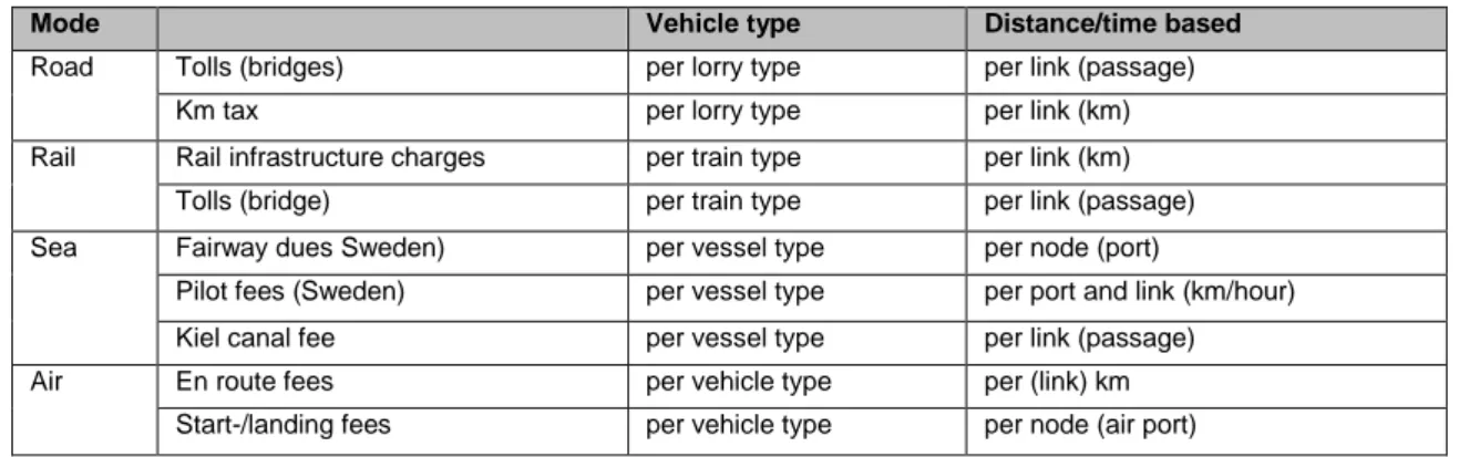
There are a total of 171 LOS-matrices, consisting of 160 vehicle specific matrices (40 vehicle types * 4 cost/time matrices) and 11 frequency matrices (where a new frequency matrix has been added for inland water way). The domestic-only distance matrices are needed for the calculation of tonkm for road rail and sea on Swedish territory, which is presented in official statistics (See section 7.2). Table 5.1 summarizes which infrastructure fees and charges are included and how they are implemented. All costs that are related to the LOS-matrices are presented in section 6 of this report.

Table 5.1 Implementation of infrastructure charges and fees. For further

details see table 6.5-6.7 and 6.10.

Mode Vehicle type Distance/time based

Road Tolls (bridges) per lorry type per link (passage)

Km tax per lorry type per link (km)

Rail Rail infrastructure charges per train type per link (km)

Tolls (bridge) per train type per link (passage)

Sea Fairway dues Sweden) per vessel type per node (port)

Pilot fees (Sweden) per vessel type per port and link (km/hour)

Kiel canal fee per vessel type per link (passage)

Air En route fees per vehicle type per (link) km

(31)

31

Another role for the network beside providing LOS-matrices is to describe restrictions that are link-based, such as the restriction that STAX 30 system trains can only use parts of the rail network that have sufficient bearing capacity. All non-link-based or node-based restrictions are dealt with in the input files via very high costs to prevent vehicle use or restrictions in nodes. As mentioned in section 4.1. there are three long train types (750 m) that are currently used in the Samgods model. The long trains are today only used for sensitivity analyses, due to

restrictions for the long trains because of too short passing tracks on the Swedish rail network. The long train types are therefore only used where double-track and/or long passing stations are available, primary within the triangle Hallsberg-Gothenburg-Malmö. Lorries with a weight of 74 tonnes are not permitted in the Swedish road network due to restrictions on how much weight the bridges can carry. Because of the restriction, the 74 tonne lorry is not modelled by default, but used in sensitivity analyses for the possibility of future changes of regulations.

5.1.1 Inclusion of extra “terminal” zones

Both the administrative zones and the possible transfer locations between vehicles need to be defined as zones in order to generate a set of vehicle type-specific LOS matrices. Therefore terminal locations such as ports, airports, lorry terminals, combi terminals, marshalling yards have been defined as additional zones. Including 464 administrative zones (discussed above), the model consists of 1 123 zones for the base scenario 2012 and 1 121 for the main scenario 2040. This means that there are 655 terminal zones for year 2040 and 657 terminal zones for year 2012. The base matrices use the same zonal numbering system as the new (domestic and international) networks.

The “terminals”, where it is possible to transfer between different vehicle types, are defined in the network (LOS matrices) as well as in the input file. The terminals are numbered according to the municipality that they are geographically located within, but with the difference that the last two digits are not “00” as with the administrative zones but in the range 01-99. In this way it is possible to see which administrative zone every terminal zone is a part of.

Table 5.2 Terminal zone numbering system by main mode

Last two digits

Road terminal zone 01-10, 51-599

Rail terminal zone 11-20

Port terminal zone 21-30

Ferry terminal zone 31-40

9_{Initially numbers 01-10 were allocated to road terminals (maximum of 10 road terminals per}

administrative zone). A later project by the National Road Administration defined a larger set of road terminals and these were then allocated the range 51-59. In the future it could be possible to re-define e.g. all road terminals to the range 51-69.

(32)

(33)

33

The figure below illustrates the different networks and how they connect.

Figure 5.1 Terminals, ports and networks

5.2 Links

All network information above, except the domestic road network, has been provided by the Swedish National Road Administration, Swedish National Rail Administration (now: Swedish Transport Administration), Swedish National Maritime Administration and Swedish Civil Aviation (now: Swedish Transport Agency) during the development of the STAN-model. The domestic road network has been extended according to an older version of the National Sampers model in order to be able to use the same road network for passenger and gods transports. There are however some parts of the logistics model that are not up to date with the current version of the Sampers model, for instance the updated speed-system. To better coincide with the Sampers model some encoding of larger objects have been done.

A link in the Samgods model is a path within the transportation network, where transportation is made. A link can for example be a road or a railroad, and can be classified by link type. This means that links can be specified depending on mode (e.g. road, rail, air, sea and ferry). Each link type has specific characteristics such as speed and are numbered according to Table 5.3. This has not direct relevance to the assignment calculation as such, but is used in the LOS-calculation as a way of defining which group of links are to be included. For example to add an extra charge on Swedish rail links but not on rail links outside Sweden.

Sea Port Sea network Rail network Road network Road Terminal

(34)

Table 5.3 List over parameters per link type.

Mode Link type Speed (km/h) Number of links

Inside Sweden

Main road links 1-69 27-111 62090

Rail links 70-79 20-86 790

Sea links 80-89 7.4–30 686

Ferry links 90-99 25 62

Road links – centroid connectors 110 50 580

Road connection links to/from terminals 201 50 788

Extra rail links to terminal zones 211 22.5–50 470

Extra sea links to port zones 221 7.4–30 148

Extra ferry links to terminal zones 231 25 34

Air 241 600 10

Total within Sweden 65658

Outside Sweden

Main road links 501-504 54-70 3034

Sea links – inland waterways 540 5 126

Extra air links to airport terminals 560 600 302

Rail links 570-579 40-72 2220

Sea links – Kiel canal 580 30 2

Sea links 581-599 25-30 530

Road connection to/from terminals 701 50 524

Extra rail links to terminal zones 711 17.5–50 278

Extra ferry links to terminal zones 721 30 142

Extra sea links to terminal zones 731 25 58

Extra air links to terminal zones 741 600 166

Road links – centroid connectors 610 50 276

Rail links – centroid connectors 678-679 17.5–49 62

Total outside Sweden 7720

Total inside and outside Sweden 73378

The link categories are related to the model, and not particularly related to the reality. In the model there are zone-centroids, which can be explained as the centre of a zone. A zone-centroid is mainly used as a simplification, where flows to different points in a zone is replaced with flows to one single point in the centre of the zone. Because of this simplification, the zone-centroid might not have physical connection to the infrastructure network. Additional links called “centroid connectors” are therefore added to the model to connect the zone-centroid to the main network. These links are defined separately from the “real” infrastructure networks. A

limitations with the zone-centroids is that it does not allow transport between the points within the zone, which are now replaced with a centroid. Another limitation is that the actual transport

Representation of the Swedish transport and logistics system in Samgods v. 1.1.

1

REPORT