Classification of Gear-shift data using machine learning

V¨

aster˚

as, Sweden

Thesis for the Degree of Master of Science in Engineering - Robotics

30.0 credits

CLASSIFICATION OF GEAR-SHIFT

DATA USING MACHINE LEARNING

Daniel Stenekap

dsp14001@student.mdh.se

Examiner: Ning Xiong

M¨

alardalen University, V¨

aster˚

as, Sweden

Supervisor: Miguel Le´

onOrtiz

M¨

alardalen University, V¨

aster˚

as, Sweden

Company supervisor: Anders L¨

ofgren,

Volvo CE, Eskilstuna, Sweden

Abstract

Today, automatic transmissions are the industrial standard in heavy-duty vehicles. However, tol-erances and component wear can cause factory calibrated gearshifts to have deviations that have a negative impact on clutch durability and driver comfort. An adaptive shift process could solve this problem by recognizing when pre-calibrated values are out-dated. The purpose of this thesis is to examine the classification of shift types using machine learning for the future goal of an adap-tive gearshift process. Recent papers concerning machine learning on time-series are reviewed. A data set is collected and validated using hand-engineered features and unsupervised learning. Four deep neural networks (DNN) models are trained on raw and normalized shift data. Three of the models show good generalization and perform with accuracies above 90%. An adaption of the fully convolutional network (FCN) used in [1] shows promise due to relative size and ability to learn the raw data sets. An adaptation of the multi-variate long short time memory fully convolutional network (MLSTMFCN) used in [2] is superior on normalized data sets. This thesis shows that DNN structures can be used to distinguish between time-series of shift data. However, much effort remains since a database for shift types is necessary for this work to continue.

Acknowledgements

I want to thank Volvo CE for providing me with this interesting topic, for the workplace, and the data that I built my thesis upon. I also want to thank my supervisor at Volvo, Anders L¨ofgren for the many hours of recording the data, for the technical expertise and support that he provided me with. I also want to thank my supervisor Miguel Le´onOrtiz at M¨alardalens H¨ogskola for the guidance in machine learning and feedback on my thesis-drafts. Finally, I want to thank my family for their patience.

Table of Contents

1. Introduction 1

2. Related Work 2

2.1. State-of-art approaches on fill-phase adaptation . . . 2

2.2. Time series classification - supervised learning . . . 2

2.3. Time series classification - unsupervised learning . . . 3

3. Problem formulation 3 3.1. Limitations . . . 4

4. Background 5 4.1. The Articulated Hauler . . . 5

4.2. Shifts and the shift process . . . 5

4.3. Machine Learning - Unsupervised Methods . . . 7

4.3.1. K-means . . . 7

4.4. Neural Network Architectures - Supervised learning . . . 7

4.4.1. Fully connected layers - the basic neuron . . . 7

4.4.2. Activation functions . . . 8

4.4.3. Drop-out Layers . . . 8

4.4.4. Long Short Time Memory Network . . . 9

4.4.5. Convolutional Neural networks . . . 9

4.4.6. Zero-padding . . . 11

4.4.7. Pooling-layers . . . 11

4.4.8. Batch Normalization . . . 11

4.4.9. Fully convolutional network . . . 11

4.4.10. Squeeze and excite layer . . . 11

4.4.11. MLSTM-FCN . . . 11

4.4.12. K-nearest neighbors . . . 11

4.4.13. Dynamic time warping . . . 12

5. Metod 13 5.1. Evaluation metrics . . . 13

6. Ethical and Societal Considerations 15 7. Methodology 16 7.1. Data collection . . . 16

7.2. Data preprocessing and feature extraction . . . 16

7.3. Supervised learning . . . 17

8. Results 19 8.1. Feature selection and K-means . . . 19

8.2. Supervised learning . . . 22

9. Discussion 25

10.Conclusions 26

1.

Introduction

Today, automatic transmissions are the industrial standard in heavy duty vehicles. Specifically, power-shift transmissions, clutch to clutch systems that shift from one gear to another without driving torque interruption, are promoted due to the increase in efficiency and driving comfort. However, tolerances and component wear can cause factory calibrated gearshifts to have deviations that affect the clutch and cause it to engage too early or too late. This causes discomfort for the driver and decreases the lifetime of the transmission.

One way to design these systems is by using a wet clutch, which is a system of oil-cooled friction discs, that transfers speed and torque through the transmission[3]. When discussing the gearshift process there are two main areas: gear-shift strategy and gear-shift control. Gear-shift strategy can be said to deal with ”when” the shift is to be made and gear-shift control can be said to deal with ”how” the shift is made. A gearshift can be divided into different phases where different control variables are relevant [3], first, the fill-phase, then either the inertia-phase followed by the torque-phase, or vise versa, depending on which type of shift that is in progress[4], [5]. The fill-phase is where the clutch cavities are filled with oil to pressurize the clutch and it is crucial, for the quality of the shift, to get this right within a close margin. Due to inconvenience (placement) and economy, commercial vehicles rarely have sensors that measure this build-up pressure, thus, getting the filling correct often comes down to factory calibration, [3]. As mentioned wear and tolerances can cause calibrations to become invalid. This means that the fill-phase becomes either too long or too short which causes over-filling or under-filling in the clutch chamber. This, in turn, affects the quality of the shift and the lifetime for the gearbox [3].

Many researchers are engaged in the topics of gear-shift control and some of the works that explore fill-phase adaptations [6], [7], [8], [9], [10], [11], will be presented in the related works section. As far as the writer of this thesis has found, no-one has explored a neural network-based approach to an adaptive fill phase. This is probably just a matter of time since machine learning is conquering domain after domain. Especially, the long short time memory network (LSTM) which is a recurrent neural network (made for time series), has had much success, like in activity-recognition [12], EEG data classification [13], chemical substance classification [14] (to mention a few).

The goal of this thesis work is to investigate fill-phase shift classification using machine learning. Some interesting work in recent times, done with recurrent neural network (RNN) in deep neural network architectures [2],[1], suggest that implementation in embedded systems are feasible. The first step towards an adaptive gear-shift process is the detection of shifts that deviate from the expected. By recognizing and categorizing these deviations adaptive measures could be taken to adjust control parameters. This thesis will compare CNN and LSTM structures in the pursuit of classifying shift data using raw and normalized data from sensors existent on commercially produced vehicles, ie. time-series data from speed, current, and pressure sensors. The work is done at Volvo Construction Equipment in Eskilstuna. At the time of writing, the targeted Volvo articulated hauler transmission has no fill phase adaptation, instead, a re-calibration is performed when required or requested. This re-calibration requires a certified mechanic and it takes the machine out of duty.

The remainder of the thesis is organized as follows: 2. related works section where state-of-art solutions to the problem formulation will be presented. Also, state-of-art applications of relevant machine learning algorithms will be presented. 3. problem formulation 4. background section where the target platform will be presented. Also, details on the algorithms, like different RNN structures, will be presented. 5. method section is where the engineering method is presented together with the expected outcome of this thesis. 6. ethics section where ethical considerations are presented. 7. methodology section where the choices made along the way are motivated. Here necessary frameworks, software, and hardware are presented. 8. results section is where the results of this thesis are presented. 9. discussion section. Here the author of this thesis argues the limitations of the work, answers the research questions, and presents future work related to this thesis. 10. conclusions section, which is a summary of the discussion and results of the thesis.

2.

Related Work

2.1.

State-of-art approaches on fill-phase adaptation

It is clear that a vehicle in use eventually succumbs to wear and tear, however, even new units are subject to production variance. Shi et al.[6] investigate which factors affect the build to build variances of transmissions. They find that torque to pressure (T2P) and pressure to current (P2I) are easily affected by several factors, among others, the hysteresis of the solenoid valve, oil com-position, and temperature as well as decay of components. They create adaptive control strategies based on the speed and timing characteristics of the shifts. Depending on the kind of vehicle, different measures can be used to benchmark shift quality. Common methods use speed or torque either from the torque converter or engine [11] [7], [8], [9], [10]. This also means that a key step is designing observers or more complete models to compensate for missing sensors. Li and G¨orges [15] design an observer from the shaft speed signals to handle unavailable variables during state feed-back control and use linear-quadratic control to create an optimal control strategy for the up-shift process of a DCT. Guo et al. [8] develops a mathematical model for a complete electro-hydraulic clutch system. They analyze the parameters with respect to stably eliminating the gap between the clutch and the piston. They find four dynamic parameters that they use for optimal control of the clutch fill. Further, they use empirical results to create an adaptive fuzzy controller that counteracts the effect of the decay of components. Using fuzzy logic controllers is also done by others with success. Wang et al. [9] use a DIDO fuzzy logic controller where the fuzzy rule set is deducted from the analysis of three unwanted states, speed drop, clutch tie-up, and engine flare. An interesting approach taken by Van Vaerenbergh et al.[10] use reinforcement learning. They use torque loss as a quality measure for the algorithm.

2.2.

Time series classification - supervised learning

In [16] Bagnall et al. compare many different algorithms for time series classification. They use the nearest neighborhood (NN) method with dynamic time warping (DTW) as a benchmark since it is traditionally one of the most popular methods. They showed that the collective of Transformation-Based Ensembles (COTE) reached state-of-art in several data sets (NN with DTW is part of this ensemble). However, being an ensemble algorithm also means that the computation time is rather long. Ismail et al. [17] note that Bagnall et al. [16] did not consider deep neural network architectures and they show that deep neural network (DNN) architecture is not significantly worse than COTE in terms of accuracy. However, due to the complexity of COTE, performance-wise, the difference should be enormous in favor of the DNN:s.

Deep learning and convolutional neural networks (CNN) have shown enormous success using images for learning complex problems [18], [19], [20], [1], since their break trough in the 2012 Large Scale Visual Recognition Challenge on the Image Net database [21]. That year’s competition was won by AlexNet, built by Krizhevsky et al. [18], which is a deep CNN architecture. Since then new deep CNN architectures were developed like GoogLeNet [19], which uses so-called inception modules and ResNet [22] which introduced an important mechanism for increasing the success of gradient descent. Long et al. [20] take inspiration from these structures and extended the concept of fully convolutional networks (FCN) and use it with great success in semantic segmentation. Wich brings us to Wang et al. [1] who use CNN architectures like the FCN and ResNet for time series classification and compare them to 1NN-DTW and COTE. Their findings indicate that a simple deep Multi-layer perception has a performance equal to 1NN-DTW and that both ResNet and FCN achieve state-of-art performance. In [17], Ismail et al review DNN:s for time series classification (TSC). They find that residual nets (ResNet) perform best with fully convolutional nets (FCN) coming second.

Recently recurrent neural networks (RNN) have also been hugely successful in a variety of areas and among the RNN:s, the long-short time memory networks (LSTM), have been a key player [23]. In [12] G¨uney and Erda¸s use a deep LSTM approach for for activity recognition. While they concede that the number of samples is somewhat lacking for some classes ins the data set, they still get an F1 score of 87.58% when learning all 7 classes from the accelerometer data. In [24] Lipton et al. compare LSTM:s against multi-layered perceptrons (MLP) with MLP trained with

hand-engineered features and find that LSTM can outperform the MLP despite only having access to raw data. While their data set is large in terms of a clinical trial, it is small in terms of machine learning, thus the need for regularization with drop out is important. In [13] Dutta performs multi-class time series multi-classification with data consists of EEG signals belonging to five different multi-classes. Using three different architectures of recurrent neural networks, standard RNN, LSTM, and GRU (Gated recurrent units)), the latter two reach an accuracy of +70%. Gleff et al.[23] analyze eight LSTM variants with the goal of understanding which design feature is most significant. The tasks are speech recognition, handwriting recognition, and polyphonic music modeling. With the use of analysis of variance (ANOVA), they find that the most important part in the LSTM is the forget gate and the activation function.

Given that both CNN and LSTM architectures perform well in TSC some attempts at combin-ing these have been made with good results. Huang et all. [25] investigate early classification in multivariate time series. They propose a combined CNN LSTM structure with parallel branches for time domain and frequency domain features called multi-domain deep neural network (MDDNN). They find that the combination of CNN and LSTM for early classification out-perform the state-of-art at that time and they credit it to the LSTM extracting temporal information from the features extracted by the CNN.

Karim et al. [26] combine the FCN with an LSTM and create the LSTM-FCN model. They reach state-of-art performance on TSC and note that the small size and efficiency of their model would make it easily deployed on embedded and real-time systems. Hu et al. [27] designing the squeeze and excite block which drastically improves the performance of DNN like ResNet by with a negligible increase in computational cost. In [2] Karim et al find the function of the SE block to be crucial for reducing the number of parameters and improving performance by giving the network a self-attention mechanism to the inter-correlation between multiple variables. With the aid of the SE-block, Karim et al. evolve the LSTM-FCN from handling uni-variate time series to multi-variate (MLSTM-FCN) and achieve state-of-art performance on a majority of the examined data sets in the UCR time-series database.

2.3.

Time series classification - unsupervised learning

The area of unsupervised learning is enormous, however since the main purpose of this thesis lies in supervised learning, only a few work will be covered here. Unsupervised learning is an important and still growing area of research, however, it does traditionally lose out in terms of accuracy to supervised learning methods [17], [1]. That being said, data does not always come with labels included.

Many types of methods deal with the clustering of time series data. Aggarwal [28] argues that the most important thing for time series clustering is the design of a similarity function. Further, he describes four shape-based clustering methods for time series: k-means, k-medoids, hierarchical methods, and graph-based methods. Ma et al. [29] note, that while k-means and k-medoids are easy to execute, they are not known for their accuracy, which in turn depends on the problem of representing a time series cluster with a distance measure. Petitjean et al [30] develop a global averaging technique, called Barycenter Averaging (DBA), to use with DTW. In [31] Ma et al. combine distance and density-based clustering (Distance Density clustering) and get a performance that is more accurate than traditional distance-based clustering and faster than fully density-based methods.

3.

Problem formulation

The purpose of the work is to take steps towards an adaptive gearshift process using machine learning. The aim of this thesis is to use machine learning to detect and classify nominal and anomalous shifts and to compare how different neural network architectures perform this task. The anomalies present in the data are overfill events in the fill-phase, ie. the phase where the initial pressurizing of the clutch takes place. An additional problem is that there exists no database from where to extract data, thus it must be constructed as a first step in the work.

Q1a How could the data set of nominal-, under-fill- or over-fill shift classes be collected and labeled for machine learning purposes?

Q1b How unsupervised learning can be used to ensure a correct labeling of the classes?

Q2 Implementations of adaptive gearshift solutions are mainly rule-based, which suggest feature engineering. Could neural networks solve this problem with raw data?

3.1.

Limitations

Due to limited time and manpower, some limitations in the work are necessary. Concerning data collection and labeling, the following limitations are made.

1. For every shift between two gears there are four different types of shift that can happen. To limit the size of the data set, only power-up shift and negative-down shift between two gears are considered.

2. Data is collected from one individual machine that is available at the Volvo CE site in Eskilstuna. Ideally, the data would be collected from several individual machines, however, due to the cost of each machine, this is unfeasible for this thesis.

3. The time factor for data collection matters. It takes roughly 15-20 min to start collecting and roughly 10-15 seconds per sample shift. Thus the final size of the data set will be limited. 4. Machine learning is a huge area. Since recursive ML-methods have had huge success in time

series classification, these will be the main focus of this thesis.

5. Due to the pandemic access to Volvo has been limited at best, which put a whole lot of additional strain on the original timetable for this thesis.

4.

Background

This section presents background on the target system, feature selection methods, the basics of the recurrent neural network architecture as well as evaluation measures.

4.1.

The Articulated Hauler

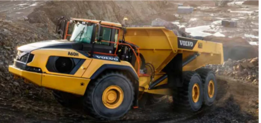
The Articulated Hauler, also known as articulated dump truck (ADT) is built for rough terrain with slippery conditions and sometimes steep inclines. Compared to rigid haulers that are able to carry much heavier payloads, their advantage lies in the terrains they can traverse. ADTs can handle terrains like swamps, marshes, and bogs at the same time as they can travel on normal roads. This makes them ideal for large construction sites where this flexibility comes into use. Currently, the world’s largest ADT, VOLVO A60H, can handle 55-ton payloads [32]. Data collection in this thesis is done on an articulated hauler.

Figure 1: An articulated hauler, which is used for data recording with the aim of an adaptive shift system.

The transmission in these vehicles is a wet-clutch power transmission that is fully automated. It consists of a torque converter with a lockup clutch connected to a planetary gearbox with eight clutches [33]. This gives a total of nine gears in the forward direction and three in reverse.

4.2.

Shifts and the shift process

There are four different categories of shifts [3], where two occurs during acceleration (power-up shift, down shift) and two occurs during de-acceleration (power-down shift, and negative-up shift).

As said stated earlier, The power-shift process in wet clutch systems can be divided into three phases [4], [5]: The ‘fill phase’, the ‘torque phase’, ‘inertia phase’. The order of these phases depends on the shift type. In power-up and negative-down shifts, the torque phase comes before the inertia phase, whilst in negative-up and power-down shifts, the order is reversed. In the torque phase, the pressurization of the clutch enables load transfer from the off-going clutch, (the configuration of the previous gear) to the oncoming clutch (the configuration of the new gear). The inertia phase is where the input speed is matched to the ongoing gear ratio (relative to the output speed) [3].

The initial pressurization of the clutch begins in the fill phase. Here the clutch cavity of the oncoming clutch is filled with oil via a solenoid valve (see Fig. 2). The inflow of oil creates pressure on the oncoming clutch by pushing the piston against the lamellae. The goal of the fill phase is to exactly hit the ’kiss-point’, which is the point in time when the cavity of the oncoming clutch has been perfectly filled and the piston has just begun to exert pressure on the lamellae. At this point, by increasing the pressure of the oncoming clutch whilst decreasing the pressure of the off-going clutch, the friction causes the lamellae to transfer torque and enables power transfer through the new configuration of the transmission and here we enter the next phase of the shift process.

While some systems use position or pressure sensors for feedback, the initial pressurization of the clutch cavity in the target machine is actuated in an open loop. Thus no feedback is available

Figure 2: Clutch layout, adapted from [33][p.18]

during the fill phase of the shift-process. This is due to having more sensors add cost and new possible points of failure [34]. Other approaches for getting the fill phase right are; direct feedback [35], using model-based observers, machine learning[10].

As stated before, the fill-time belongs to a set of pre-control variables that are set via empirical calibration methods. This is a common approach among commercial manufacturers [3]. This can be illustrated by Fig. 3.

Figure 3: Shift control strategy using adaptation and precontrol from [3][p.217]

The initial calibration is based on sample mean and fits well with the majority of the produced transmissions, however, for some individual transmissions, additional calibration might be needed. Correct settings are important since under- or overshoot with respect to clutch filling affects the total quality of the shift as well as the expected life of the transmission.

Problems that can occur during the fill phase are under-fill and over-fill of the cavity [8]. The reason for these events can depend on several factors, like, a drop in oil pressure, clutch lamella wear or, outdated pre-calibration values. Indeed, due to production tolerances and component wear, individual gearboxes may drift away from predefined optimal calibrations. Dai et al. showed that 30% of the automatic transmission in their sample were in need of shift adaption. The effect of these events transfers to the next phase in the shift process. For instance, A power-up shift under-fill scenario: The clutch has not been properly filled and once the torque phase begins, some of the oil pressure that should have gone towards pressurizing the clutch is wasted on filling the remainder of the clutch cavity. This results in engine flare as the friction in the clutch is unable to absorb the torque of the off-going clutch. Engine flare increases heat in the clutch and can lower the life expectancy of the clutch[8]. Another example is a power-down shift over-fill scenario: The clutch is pressurized ahead of time and in the inertia phase, the off-going clutch does not disengage properly. This results in clutch tie-up and will cause the vehicle to suffer traction loss [36]. Thus

there are very real gains in having a system that can continuously adapt the shift process during everyday operations of a heavy-duty construction vehicle.

4.3.

Machine Learning - Unsupervised Methods

Unsupervised learning models use underlying structures in the data to group it into clusters or recognize anomalies. They are also referred to as model-based or as generative models [1]. Further, Wang et al. argue convincingly that these methods are not often competitive with supervised methods nor are they meant to be used as end-to-end classifiers [1] which is echoed by [16]. For this reason, the focus has been shifted to one simple method (k-means) to give support for the prepossessing step.

4.3.1. K-means

K-means clustering is a method that partitions a set into clusters by assigning k ”means” to the data set. These means can also be referred to as centroids. The number k is selected as the expected number of classes for the data to be partitioned into. The algorithm follows the following steps:

0. Initiate the k-means by some method like Forgy or Random Partition [37].

1. Assign each observation to a cluster according to some distance measure, like euclidean. 2. Update the k-means by calculating the means of each cluster

3. Repeat from 1.

Thus k-means is trying to minimize the within-cluster variance as can be seen in equation 1

argmin S i=1 X k X x∈Si ||x − ui||2 (1)

where Si is the i:th cluster, x, is a sample in that cluster and ui is the i:th cluster mean. While

K-means can be adapted to time series, it is better used with a feature-based approach as it would make assumptions like one-to-one correspondence between time points and time series having the same length [28].

4.4.

Neural Network Architectures - Supervised learning

Supervised methods rely on labeled data sets for training. A neural network is a machine learning technique inspired by the neurons of our bodies. While research in the area begun already in the 50s [38] it took quite a few years until the first recurrent neural networks were proposed. They first surfaced in the 80s after the famous article on Backwards propagation by Rumelheart[39], but their real success comes even later. CNN architectures began seriously developing after the article by Lecun et al [40]. One way to consider Artificial neural networks (ANN) is by stacking different types of layers that transform input-data as it passes through them. With this abstraction, there are numerous types of layers. The ones that are used in this thesis will be explained in the following subsections. When an ANN is used as a classifier, the final layer will output the probability of the data belonging to a certain class. Un-referenced claims in this subsection are adapted from the textbook Neural Networks and Deep Learning by Aggarwal [41].

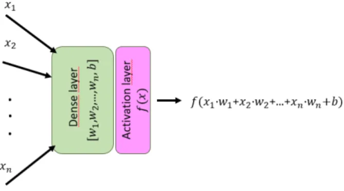
4.4.1. Fully connected layers - the basic neuron

The fully connected layer or dense layer consists of an array of neurons matching the dimension of the input data. A neuron is made up of a weight vector with a weight for each of the incoming connections and a bias value. The input goes through element-wise multiplication with the weights

and is added the bias value. Finally, it is sent through an activation function. The equation for output from a single neuron can be formulated as follows

output = f (

n

X

i=1

wiXi+ b) (2)

where f is some activation function, Xi is the i:th connection in the input vector X, wi is the

weight for the i:th connection and b is the bias of the neuron (see figure 4). A Dense layer consists of several neurons and is associated with a weight matrix and a bias vector.

Figure 4: The data flow through an simple neuron can be described as follows. The input vector is element wise multiplied with the weight vector in the neuron. Then bias is added and the sum is sent to the activation layer where an activation function completes the output.

For more in-depth information, see chapter 1 in [41] by Aggrawal or the article by Zhou at [42]. 4.4.2. Activation functions

When data passes through neural networks, it’s the activation functions that add non-linearity. The functions that are used in this work are the sigmoid function (σ(x))

σ(x) = 1

1 + e−x (3)

the tanh function

tanh(x) = e

x_{− e}−x

ex_{+ e}−x (4)

ReLu function

ReLu(x) = max(0, x) (5)

and the SoftMax function,

Softmax(xi) =

exp(xi)

P

jexp(xj)

(6) which outputs a vector which corresponds to the number of classes. Here, j sums over the number of output classes, and xi will result in the probability for the i:th class. A good explanation on

the SoftMax layer is made by Zhou at [43]. 4.4.3. Drop-out Layers

A drop out layer is a layer that randomly mutes connections during training. It has the effect of preventing overfitting during training.

4.4.4. Long Short Time Memory Network

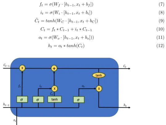
In 1997, a new kind of recurrent neural network was introduced in the paper by Hochreiter and Schmidhuber[44] called Long Short Time Memory (LSTM) network. LSTM:s are able to connect features through very long time lags and have been successful in many areas as will be presented later in the related work section. For a comprehensive and step-by-step explanation of the LSTM, the reader is referred to a blog post by Christopher Olah, [45] or chapter 7.5 in Neural Networks and Deep Learning by Aggarwal[41].

LSTM:s use a structure with memory cells and gate units. First, define xt, Ct and ht as

the input vector, cell state vector, and hidden state vector at time t. Also, define W as the weight matrix, b as the bias vector. Now, the information flow through an LSTM-cell used three ”gates”. The forget gate, which decides how much of the previous state is to be retained. It is based on the concatenated previous hidden state and current input. The input gate, based on the concatenated previous hidden state and current input, decides how much the current input will affect the current state. Finally, the output gate, based on the current state filtered through the concatenated previous hidden state and current input. At each recursion, the input to a LSTM cell is xt, Ct−1and ht−1 and the output is Ct and htwhere the final hidden state corresponds to the

classification. The equations are as follow are adapted from [14] and the ’∗’ denotes element-wise multiplication. ft= σ(Wf· [ht−1, xt+ bf]) (7) it= σ(Wi· [ht−1, xt+ bi]) (8) ˜ Ct= tanh(WC· [ht−1, xt+ bC]) (9) Ct= ft∗ Ct−1+ it∗ Ct−1 (10) ot= σ(Wo· [ht−1, xt+ bo])) (11) ht= ot∗ tanh(Ct) (12)

Figure 5: A flowchart of an LSTM cell. The green rectangles represent layers while the yellow circles represent point-wise operations. C is the cell state, x is the input, h is the hidden state. See equations 7- 12 for details. This picture was adapted from [45]

4.4.5. Convolutional Neural networks

Convolutional neural networks (CNN) are most known for their success in the field of computer vision, where the architectures are often deep and complex, however, they can also handle time series [46]. This can be done either by representing the time series as an image and using 2D or 3D convolutions, which requires some preprocessing of the time series. There is also the alternative to do 1D convolutions which has the advantage of allowing the time series to be feed directly into the network with minimal preprocessing (FCN architecture in [1] for example).

For an in-depth explanation of the CNN type networks, the reader is referred to chapter 8 in Neural Networks and Deep Learning by Aggarwal[41] or a more intuitive explanation in the online article [47].

A CNN is built by stacking several different layers together where the convolution layer is the defining one. Each convolution layer has a number of K filters with randomly initiated weights. For a given layer the width v, of these filters are the same, usually an odd integer. The width is commonly referred to as the kernel when the dimension is leq 1. A 1D convolution operation is performed by sliding filters along each position of the time series, ie. through time. The purpose of the filters is to extract features from the time-series and the output of every filter in a convolution layer is called a feature map. A time series with length m will after each successive convolution layer, decrease in length with bm − v + 1c. Now, lets consider a vector X with c channels, ie. X = [x1, x2, ..., xc], sampled into a discrete time series S with length m as S = {X1, X2, ..., Xm}.

A filter d in a convolutional layer will have the dimensions v × c, where v is the filter width, and c corresponds to the number of channels of the time series. Letting S be the input to a convolution layer with K filter of width v, then the output can be defined by

f (S) = f (X1, X2, ..., Xm) =

= f₁(1), f₂(1), ...f_K(1), f₁(2), f₂(2), ...f_K(2), ..., f₁(bm−vc+1), f₂(bm−vc+1), ...f_K(bm−vc+1) (13) where output from the k:th filter centered at the n:th time step is defined by

f

= σ(

X

X

X

d

+ b

)

(14)

where bk is the bias for the k:th filter. To illustrate this with an example, in figure 6, a time

series with 4 channels is convoluted with a single filter of width 3 and produces a single output for every one of the remaining bm − vc + 1 time-steps.

Figure 6: A time series and a filter with width 3 are shown in the left box. In the middle box, the filter and the time series are aligned for convolution. In the right box, the output of 1 time step is shown.

The features outputted from the convolution operation increased the dimension of the output compared to the input. When stacking multiple convolution layers, the number of feature maps would quickly grow large, which requires more computational power. Selecting the number of filters and their width depends on the task, the optimal number of filters and their length varies and the common way to do this is by trial. In [46] they find that a filter length of 7 is best suited for their task. Setting the number of filters to a power of 2 is computationally efficient [41].

4.4.6. Zero-padding

Zero-padding is a technique that adds zero values to the start and end of inputs (all around it in case 2d and 3d inputs). With convolutions, the number of zeroes is taken as half the width of the filter rounded up. This deals with data loss around the edges of the input and it can also be reapplied in later convolution layers. With RNN:s zero-padding can be applied to equalize the length of the time-series by adding zeros at the end of the shorter series.

4.4.7. Pooling-layers

Pooling layers solve the problem of convolutions increasing dimension, as well as, introduce non-linearity to the model. The pooling operation can be considered something like a convolution in reverse. There are different kinds of pooling, like max-pooling and average-pooling, and can be read about in chapter 8.2.5 in [41] by Aggrawal. In this thesis, only global-pooling will be applied. It works by selecting the maximum value from each feature map, ie reducing dimension from [bm − vc + 1 × K] to [1 × K].

4.4.8. Batch Normalization

Batch normalization is a technique that normalizes the output matrix from a layer and is often used in combination with convolutional layers. By normalizing activations inside the hidden layers training speed is increased and it has an effect similar to dropout layers on the CNN networks [48]. In [49] Ioffe et al. achieve 14 times reduction in training.

4.4.9. Fully convolutional network

In [1], wang et al. find that the FCN network performs well when classifying time series. A more in-depth explanation of the FCN can be found in [20]. The structure consists of three stacked blocks, each consisting of a 1D-Convolutional layer, batch normalization layer followed by ReLu activation. This means that the features from the 1D convolution are normalized and then the negative values are set to zero. After these blocks, there is a global pooling layer and finally a fully connected layer with SoftMax.

4.4.10. Squeeze and excite layer

The squeeze and excite (SE) layer proposed by lang et al. [27] takes a convolution block as an input. It used max-pooling to reduce (squeeze) each of the K feature maps for that block with size c × v (c is the spatial dimension of the input) into a vector where each dimension is represented by a single value c × 1. Then it uses a fully connected layer with ReLu and a reduction ratio to add non-linearity and reduce complexity. The SE layers have been shown to substantially increase accuracy [27], [2] of models while only adding a slight increase to parameters (3-10% [2]). For a more in-depth explanation see the original work of Lang et al in [27] or the article by Pr¨ove at [50]. 4.4.11. MLSTM-FCN

As described by Karim et al in [2], the model of the MLSTM-FCN is built using an FCN in parallel with an LSTM. The input enters an FCN branch that is built by stacks consisting of a convolution layer followed by batch normalization and a ReLu before going through an SE layer, see fig. 7. An adaption has been made to the MLSTM-FCN by adding a masking layer to deal with zero-padding on the LSTM branch. A masking layer lets the network know that time-steps are missing in the data.

4.4.12. K-nearest neighbors

K-nearest neighbor is a simple supervised classifier. Given a new input, the KNN algorithm searches the known (labeled) data for the K most similar points (according to some distance measure) and returns the majority label. The advantage of this method is the simplicity however with large data sets, the computational cost becomes high since for, each input, the distance to all points in the

Figure 7: MLSTM-FCN adapted from [2]

data set needs to be calculated. In the context of time series classification, the KNN algorithm is often used with the dynamic time window (DTW) similarity measure as a baseline comparison, like in [1].

4.4.13. Dynamic time warping

The DTW measure is good when comparing time series. For two samples A and B, with equal length N , it is computed by moving from the start of time to the end of time while calculating all the distance between Ai and Bj. These distances are then stored in a matrix and the shortest

cumulative path from A0, B0 to AN, BN, is the DWT measure. This way DTW produces the

optimal nonlinear alignment between the series. This method in combination with the 1-nearest neighbor’s algorithm has been dropped from implementation due to how expensive it is to train and since DNN structures have similar or better performance [1].

5.

Metod

In this thesis, the process is outlined by Charu C. Aggarwal in [51], has been adapted.

Data

collection

extraction

Data preprocessing

Analytical

preprocessing

Feedback

Feedback

Output

The data procesing pipeline

Figure 8: The data processing pipeline adapted from [51][p.4]

It starts with data collection which is highly platform-dependent and often done without the in-volvement of the data analyst. For data sets that need closer examination before given annotations, feature extraction and data cleaning are used to aid the process. Generally, feature extraction is used to make the mining process more efficient and data cleaning, for example, removal of outliers and addressing missing values, is often crucial for good results. Finally, the data set can be reduced through feature selection and transformed for further machine learning. At this point, the data set will undergo training in different machine learning models. Before training, the data set is split into a training set and a validation set. The models have different hyper-parameters that can be tuned for improved results as well as to avoiding overfitting the model to the data. It is common to iterate over the steps in this process as new problems can be discovered at a later stage. Once a satisfactory result has been achieved with machine learning, a prototype can be designed tested on the intended target.

5.1.

Evaluation metrics

To evaluate the learning methods, the following metrics are used. A True Positive (TP) is scored when the prediction matches the data label, a False Positive (FP) is scored when the prediction fails to predict a specified data label and finally, a False Negative (FN) is scored when the prediction falsely predicts a specific data label.

1. Confusion matrix:

Actual

Positive Negative Predictions Positive True Positive False Negative

Negative False Positive True Negative

From the confusion matrix a number useful measures can be computed like: 2. Accuracy:

Accuracy = T P + T N

T otal (15)

3. True positive rate, also known as recall:

Recall = T P

4. Precision:

P recision = T P

T P + F P (17)

5. F1-score, which is the harmonic mean of the recall and precision: F1= 2 ·

P recision · Recall

P recision + Recall (18)

These metrics are commonly used in papers and in articles and some of the papers cited in this thesis use them, for example, [12].

6.

Ethical and Societal Considerations

The source of the data signals as well as the intended future target system belongs to Volvo Con-struction Equipment. Since signal data and some specifications of the conCon-struction vehicle are confidential, signals are named only with general terms, and specifics concerning features are left vague on purpose. No data besides the results are presented.

7.

Methodology

7.1.

Data collection

The first step in the process of designing adaptive shift control is to procure a data set. At the start of this thesis, there exist no such data sets at Volvo CE. This is a major difficulty since data collection is a time-consuming process and in addition, there is the annotation of data for ground truth, which is required for supervised learning. As mentioned earlier in the background, the data is collected from an articulated hauler and consists of, in total, 20 channels sampled with 100 Hz. The data set contains shaft speed information and shift-state information that has been time-stamped. A recording is made by having a driver connect a laptop running ATI Vision 5.2.1 software to the engine control unit (ECU) of the dumper via an A8 Serial ECU Interface module. The ECU directly provides system state information, while sensor data is transported via CAN bus. This means that there are two different clocks involved in the data sampling and there is no synchronization between them. To record the nominal state a set of pre-calibrated ’optimal’ parameters were used. These parameters are then shifted accordingly to create the underfill and overfill scenarios. The driver then proceeds to drive on the test track that they use at the site at Volvo CE Eskilstuna.

The first recordings were made on a velodrome where the driving conditions basically can be assumed to be: flat ground with no wheel slippage. After making the first recording, a discrepancy in the size was discovered in between the samples originating from the sensors contra the samples containing state information. It was theorized that the lack of synchronization might cause this and that restricting the time length of each recording to around 5-6 min would reduce the problem. Another data set was recorded in a rougher setting where the track consists of muddy uneven ground over a hilly landscape. With this setting, the number of samples in the correct shift categories decreases however, the signal data is much more realistic. Due to corona, collecting data became a problem, and in the end, the underfill category was dropped.

As mentioned earlier, the data is recorded by manipulation of a set of parameters. However, even though a recording is made with a parameter set that would produce a certain category of shifts, all shifts in that recording might not share those characteristics. This is due to system variables subjected to noise and drift which can be offsetting the optimal calibration, or affect the sensor readings. Since it’s important for machine learning purposes that the data set has the highest possible quality, to aid the annotation of the data an additional sensor (pressure), which is unavailable in the commercially produced vehicles, is included for prepossessing purposes.

7.2.

Data preprocessing and feature extraction

Thanks to restricting the recording length to a 5-6 min interval, the differences in lengths between the different groups in the data set was brought down to about 4 samples out of 72 000. The small differences in the size of the samples are resolved by using linear downsampling to the shortest of the sample lengths. This is only a problem for the pressure signals which are used for feature construction since they differ from the shaft speed signals which will be used for supervised learning. From the collection of recordings, shifts that fit the criteria were extracted and put into the data set that is henceforth referred to as raw data set. A copy of this data set was normalized and is referred to as the normalized data set. Finally, a copy of both normalized and raw data sets was intersected with the k-means results forming the pruned-raw data set and the pruned-normalized data set.

For the labeling of the data set, experts at Volvo showed how the values from the pressure sensor formed a bubble over the requested pressure signal when overfill occurs. This could be seen as an area feature between the requested pressure signal and the pressure signal at a time interval revolving around the point of contact between the friction lamellae of the oncoming clutch. How-ever, after examining the data, it was found that the bubble feature could not explain overfilling in a large number of samples, this was especially true for the down-shifts. Even when the feature indicated a nominal shift, human experts could confirm artifacts in the shaft speed signals, indicat-ing that overfill had indeed occurred. While it would seem that the sensor would give the ground truth of the pressure level inside the transmission, the location of this sensor is asymmetric in regard to the different gears that are involved, thus for some gear-shifts, it will give more accurate

readings due to having a placing closer to the operated fill chamber. It should be mentioned that at this point, the data set consists of 4000 samples of extracted shifts. There was no way to have a human expert going through all those, other methods were needed.

This brought the idea of using unsupervised learning to verify the recorded classes. For this purpose, features were created and analyzed and selected for use in a K-means classifier. First, the shift data were grouped into up-shifts and down-shifts. The pressure sensor data was then filtering with a Butterworth filter setting normalized cutoff, N C = 1 which corresponds to a cutoff frequency (CF) of 50 Hz (recomended by experts at Volvo) and the filter is created with the Matlab function designf ilt() to remove noise on the signal. Different features, both in the time-domain and frequency-domain, were created on the pressure sensor data and examined in different time intervals around the kiss-point. After feature selection, the data was normalized and used in K-means for classification. An intersection of the K-K-means clusters and the original data set was used to create an additional ’pruned’ data set for comparison.

It should be mentioned that other clustering methods were initially attempted but dropped due to poor results (Dirichlet process infinite Gaussian mixture model) and time restraints (maximum a-posteriori Dirichlet process mixtures).

The preprocessing step is made in Matlab 2020a.

7.3.

Supervised learning

Four shaft speed signals were used for the supervised learning and four neural network models are used on this problem, an MLSTMFCN by [2], the FCN, the LSTM, and a CNN. All networks use: Adams optimizer (initial learning rate, lri, = 1e−3 and final learning rate, lrf= 1e−4), Categorial

cross entropy loss function and fully connected SoftMax output layer (two classes). The list below describes parameter choice’s for the employed networks. This is a result of an iterative trial and error process over many parameters like filter size, filter width, number, and type of layers. For further details on specific networks, see section 4.4. or the references listed therein.

I The structure of the MLSTMFCN follows the description in section 4.4.11. see fig7 with parameter choices below.

Fully convolutional branch: three FCN layers, (filters=128,width=5), (filters=128,width=7), (filters=256,width=7) were the last lacks SE layer.

LSTM branch: zero-masking layer, LSTM-layer with 128 units followed by a dropout layer set to 0.2.

II The structure and parameters of the FCN are the same described in [1] except it has no global-pooling layer.

III The structure of the LSTM follows the LSTM branch of the MLSTMFCN but with twice as many units (256) in the LSTM-layer.

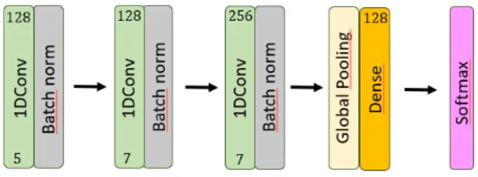
IV The structure of the CNN can be seen in figure 9 with parameters as below:

1D convolution layers (filters=128,width=5), (filters=128,width=7), (filters=256,width=7) each followed by batch normalization. Then global pooling into a fully connected layer with 128 units, see figure 9.

Figure 9: The structure of the implemented CNN

All networks train over 100 epochs with a batch size of 32 (16 and 64 were tried but 32 was better). The data is randomly split 70%/30% training to validation and all networks train on the

same split. No sliding window is applied since the shifts have already been extracted during the preprocessing step and the individual sample lengths are relatively short. Since the shifts-samples are of different lengths, zero-padding was applied to bring them all to equal length. This is the reason for the adoption of masking layers previously stated in section 4.4.11.

For the supervised learning part, Python 3.8 with Tensorflow 2.1 functional API, sci-kit-learn 0.23.2 is used. The development environment is Jupyter lab 2.2.6.

8.

Results

In this section, results from the different parts of the thesis work are presented. The motivation of the selected features and results from the k-means clustering from unsupervised learning. Training graphs over accuracy and loss over raw and normalized data sets as well as training time and model size are presented for supervised learning.

8.1.

Feature selection and K-means

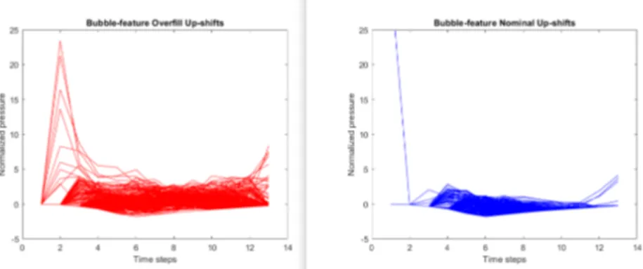
Returning to the preprocessing of the data, feature extraction and selection was necessary for k-means. The first feature that was suggested by experts at Volvo was the bubble feature. In figure 10, it is shown how the pressure spikes on the overfill up-shifts, however for the down-shifts (figure11), the pressure spike is not larger but time shifted.

Figure 10: The ’bubble’ feature, normalized over up-shifts is a increased pressure spike compared to nominal up-shifts

Figure 11: The ’bubble’ feature, normalized over down-shifts is a time shift compared to nominal down-shifts.

This means that the feature must be differently constructed for up-shifts and down-shifts. A normalized histogram show how nominal and overfill shifts overlap (figure 12). This is expected and the feature provides decent separation for up-shifts in most samples with an overlap of less than 30%. When examining the down-shifts, however, separation is not as good as about 50% of the overfill data overlaps with the nominal (figure 12).

New features could improve separation. Given the purpose of the thesis and the scope of such task, it was deemed sufficient, if a few such features, capable of separating the category’s, could be found.

The first considered feature was fitting a line to the part of the sample where the area bubble might begin. The idea is that the slope of that line would differ for overfill shifts compared to nominal. Targeting the time shift for down-shifts, a short time interval is fitted with a line using Matlab function f it(). For the up-shifts, targeting the beginning of the spikes, a slightly longer

Figure 12: While the ’bubble’ feature separates decently with about < 30% overlap, between nominal and overfilled up-shifts (left), the result for downshifts (right) with ∼ 50% overlap is much worse.

interval is again fitted with a line using Matlab function f it(). The results suggest decent separation as seen in figure 13.

Figure 13: The ’slope’ feature captures a difference between nominal and overfilled shifts. Up-shift (left) and down-shifts (right).

In addition to this handmade feature, mean value, skew, and standard deviation were consid-ered. The time domain features are presented for up-shifts in figure 14 and for down-shifts in figure 15. Standard deviation was the feature offering the best separation and it was also the last feature selected for input to k-means clustering.

Figure 14: Histograms of the features; mean (left), standard deviation (middle) and skew (right) for nominal and overfilled up-shifts

Attempts at simpler frequency domain features, like mean frequency and power were made but they did not provide enough separation (figures omitted). A comparison of stacked single-sided amplitude spectrum plots from nominal recordings and overfill recordings show that hand engineering features might be possible but given promising results from the time domain, this is left for others to explore (figures omitted).

To summarize; three time-domain features were selected, pressure difference, standard devia-tion, and slope. Both pressure difference and slope are hand-engineered from a knowledge of the

Figure 15: Histograms of the features; mean (left), standard deviation (middle) and skew (right) for nominal and overfilled down-shifts

signal and differ for up-shifts and down-shifts.

Once the features were selected, they were normalized and fed to Matlab’s K-means algorithm. The results from the K-means show that the algorithm with the selected features cluster most samples, both for up- and down-shifts, to the recorded categories (figure16). K-means reach an accuracy of 98.4% for up-shifts and 91.9% for down-shifts. At this point, an intersection between the K-means clusters and the recorded clusters is created for comparison for supervised learning. The k-means algorithm is run a second time on this intersection which results in nearly clean sets (see figure17).

Figure 16: First K-means clustering shows some samples assigned to a different cluster compared to what the data would indicate. The dots are the K-means clusters and the ring-frames are the initial annotations given from recording settings. The down-shifts (right) have a larger portion of samples where K-means disagrees with initial labels.

8.2.

Supervised learning

The supervised learning methods were trained only on shaft speed signals and are independent of the pressure sensor which was used for the unsupervised learning. The accuracy results using training and validation sets together sets can be seen in figure 18.

Figure 18: Table over accuracy on whole data sets. Green fields are best results while red fields indicate failure to train.

The most successful models on all data sets were the MLSTMFCN and the plain LSTM. Both models manage to train on almost all data sets with the raw up-shift data being the hardest to learn. While the MLSTMFCN scored a bit higher over the sets, it also took longer to train. The average training time for the MLSTMFCN implementation was 420 s on up-shift data and 327 s on down-shift data while the LSTM took 116 s and 107 s respectively. The number of trainable parameters for the MLSTMFCN is just below 500 000 while the LSTM has about 415 000. Both networks get accuracy scores of around 81 − 85% on validation data set for normalized up-shifts and around 93 − 96% on validation set data for normalized down-shifts. The results calculated on the confusion matrix on validation data for the MLSTMFCN after 100 epochs on normalized up-shift and downshift data can be seen in figure 19.

Figure 19: Precision, recall and F1-score calculated from the confusion matrix on validation data for the best model on normalized original data set

It was hard to make the FCN train on the data sets. The width and sequence of filters mattered, as well as, removing the global pooling layer. This resulted in the adapted network described in 4.4.9. The size of the network is the smallest of the models, with about 325 000 parameters. The FCN sometimes manages to train on raw up-shift as well as on raw down-shifts but far from consistently. This has probably to do with the weight initiations as they are the only parameters that change from iteration to iteration. In figure 20 an example of how the network successfully starts training on raw up-shift data is shown. It reaches an accuracy of +86% which is better than the networks with the LSTM cells. Then something happens around the 90:th epoch and the training abruptly worsens. However, with access to the accuracy and loss graphs, and as it is easy to save weights during training iterations, this is not a big problem. The best combined results on raw data were achieved on the FCN.

The CNN network was hard to tune on the data sets, except on normalized down-shift data. Several combinations of filter lengths using the three stacked convolutional layers were tried as their order had made a big difference for the result of the FCN. The global pooling layer was also

Figure 20: The training graph for the FCN where training accuracy abruptly falls after about 90 epochs.

removed and replaced with a flatten layer but this did not make a difference. The CNN consistently failed to train on any raw data and only scored close to 65% on the normalized up-shifts.

For all networks, there are several possible explanations for underperformance. The choice of preprocessing that was employed in this thesis where the networks learn temporal features without a sliding window, might be an issue. Or it might be that a key feature in the data, is missed due to parameter choices like the number of layers and filter sizes and lengths.

For the supervised learning algorithms, up-shift data was harder to learn than downshift data. In fact, for all sets and models, learning down-shifts resulted in higher accuracy compared to learning up-shifts. To illustrate this figure 21 compares the training graphs on up and downshifts, on the most successful model, on the normalized data set.

A reason that down-shifts are easier to learn might be the sample length which is longer for up-shifts than for down-shifts. However, after consulting with experts on Volvo, a likely reason is that overfill on negative down-shifts has a higher impact on the shaft signals compared to power up-shifts.

Out of all models, only the plain LSTM model consistently managed to converge on the (up-shifts) raw data set, even though the accuracy could not compare to the normalized set (illustrated in fig. 22 It is clear that normalizing a data set helps the training process a lot as all models performed much better on the normalized data set compared to the raw.

As a final note, the effect of pruning the data sets with the k-means intersection make the up-shift data harder to learn, but slightly improves learning on down-shift.

Figure 21: The training graphs for the MLSTMFCN on the normalized up-shift and down-shift sets, where, like on all other sets, the down-shift training results in higher accuracy.

Figure 22: LSTM - raw up-shift vs normalized u-shifts. The training shows the same trend but with much worse results for raw data compared to normalized

9.

Discussion

A data set with nominal and overfilled shift was created and to validate the data set, feature extraction, and the selection were done on the pressure signal, a signal which is unavailable on commercial vehicles. The two hand-engineered features in combination with the standard deviation resulted in the k-means algorithm clusters which coincided with the recorded classes with high accuracy. This can be taken as a strong indication of the validity of the data set. It would be interesting to use clustering methods on the shaft speed in time-series format. Unsupervised methods that employ DTW like hierarchical clustering would be necessary since k-means does not deal well with time-series [28].

The idea of pruning the data set with the intersection of the recorded labels and the k-means clusters had the intention of improving the data set for supervised learning. In hindsight, there is little support that removing shifts based on features created from the pressure sensor would remove outliers since no connection between these features and potential outlier was investigated. In fact, no investigation of outliers was made besides taking precautions for shifts following each other too close in sequence. Since outliers have a disproportionate effect on learning [28], this merits consideration. There are unsupervised methods for outlier removal that could have been applied and then hand-checked, but this is left for future work.

The results from the feature selection and unsupervised learning gave some indication that the down-shift might be harder to learn than the up-shift since the pressure sensor readings were harder to interpret for down-shifts. However, after discussing with experts at Volvo, there was a clear explanation for the down-shift being easier to learn. The shaft speed are more affected by the overfill during the down-shift. The reason is that the downshift is performed while coasting, thus the input torque is low, the off-going clutch then starts to slip due to the torque peak in the ongoing clutch during the overfill. In the up-shift, the input torque is around 8-10 times higher. The off-going clutch is then held with a corresponding higher torque. The torque peak caused by the overfilling clutch is not enough cause a larger slip in the off-going clutch.

In this thesis, two of the four shift types were considered, also, these shift types were limited between two gears. Since the targeted system has nine gears in the forward direction, a lot of work remains to be done in order to collect data sets for a database containing labeled shift types for supervised learning.

Three of the four models performed well on the data set and while all models managed to train on the raw data, the FCN had the best-combined accuracy both up-shifts and down-shifts. On the normalized set, the MLSTMFCN had the best combined accuracy. Over-fitting is detected by comparing training and validation accuracy or comparing training and validation loss. From the graphs in figures 20,21, it can be seen that the validation loss and accuracy are sticking close to the training loss and accuracy, which is a good indicator of generalization (no over-fitting). Since the FCN is the leanest of the models in terms of the number of parameters, it would be the first choice for a targeted embedded system. The results from the supervised learning prove that it is possible to design an adaptive shift process based on machine learning but there remain many steps to be taken.

It was very hard to train the CNN model on the data sets. What helped the FCN perform was surprisingly the removal och the global pooling layer. This might be a clue to the poor performance of the CNN. It might be that too many features were generalized in the global-pooling step. In future works, a different approach to pooling might improve results.

10.

Conclusions

This was a first attempt at creating a data set for nominal and overfilled shifts on the articulated hauler transmission. It is clear that many things could have been done better. A more complete methodology for determining the validity of the data set is a good starting point for further work. A larger data set is always good when working with machine learning. However, this work shows that unsupervised methods like k-means can be used to verify the validity of the recorded labels with some feature engineering on pressure sensor data. The k-means method using the selected features clustered 98.4% of the up-shifts and 91.9% of the downshift to the same categories that were recorded. Using this kind of approach could save manpower hours on larger data sets.

Before a complete model can be trained, the data set would need to be expanded to cover all shift types and probably more gears. Also, as the overfill-data was generated by setting a constant offset to the fill-time, the offset limit in respect to what could be recognized as an overfill event should be investigated. In this work, four DNN architectures were trained the shift data set. The FCN, MLSTM, and the LSTM all showed a strong performance on the data sets, even though they sometimes failed to train, this can be resolved by focusing on one determined model. The FCN had the best combined performance on the raw data set with 86.18% accuracy on up-shifts and 92.09% accuracy on downshifts, and it has the least amount of parameters. This would be the model of choice for further work towards an adaptive shift process using machine learning if preprocessing of the data is not possible. The best combined accuracy on the normalized data set was achieved by the MLSTMFCN model with 91.22% on up-shift and 97.62% on downshift data so this would be the method of choice if the model size fits and normalization is can be implemented.

References

[1] Z. Wang, W. Yan, and T. Oates, “Time series classification from scratch with deep neural networks: A strong baseline,” in 2017 International Joint Conference on Neural Networks (IJCNN), 2017, pp. 1578–1585.

[2] F. Karim, S. Majumdar, H. Darabi, and S. Harford, “Multivariate lstm-fcns for time series classification,” CoRR, vol. abs/1801.04503, 2018. [Online]. Available:

http://arxiv.org/abs/1801.04503

[3] R. Fischer, The Automotive Transmission Book, 1st ed., ser. Powertrain. Cham: Springer International Publishing, 2015.

[4] T. Zhang, G. Tao, and H. Chen, “Research on fill phase control strategy of shifting clutch,” in Proceedings of 2011 IEEE International Conference on Vehicular Electronics and Safety, July 2011, pp. 34–38.

[5] F. Gustafsson, “Wet clutch load modeling for powershift transmission bench tests.” Master’s thesis, Karlstad University, June 2014.

[6] G. Shi, P. Dong, H. Sun, Y. Liu, Y. Cheng, and X. Xu, “Adaptive control of the shifting process in automatic transmissions,” International Journal of Automotive Technology, vol. 18, pp. 179–194, 02 2017.

[7] Z. Dai, P. Dong, and W. Guo, “Adaption strategy of power on down shift for automatic transmission,” in 2016 35th Chinese Control Conference (CCC), July 2016, pp. 9005–9009. [8] W. Guo, Y. Liu, J. Zhang, and X. Xu, “Dynamic analysis and control of the clutch filling

process in clutch-to-clutch transmissions,” Mathematical Problems in Engineering, vol. 2014, pp. 1–14, 06 2014.

[9] S. Wang, Y. Liu, Z. Wang, P. Dong, Y. Cheng, X. Xu, and P. Tenberge, “Adaptive fuzzy iterative control strategy for the wet-clutch filling of automatic transmission,” Mechanical Systems and Signal Processing, vol. 130, pp. 164 – 182, 2019. [Online]. Available:

http://www.sciencedirect.com/science/article/pii/S0888327019303097

[10] K. Van Vaerenbergh, A. Rodriguez, M. Gagliolo, P. Vrancx, A. Nowe, J. Stoev, S. Goossens, G. Pinte, and W. Symens, “Improving wet clutch engagement with reinforcement learning,” 06 2012.

[11] T. Zhang, G. Tao, and H. Chen, “Research on fill phase control strategy of shifting clutch,” 07 2011.

[12] S. G¨uney and C. B. Erda¸s, “A deep lstm approach for activity recognition,” in 2019 42nd International Conference on Telecommunications and Signal Processing (TSP), 2019, pp. 294– 297.

[13] K. K. Dutta, “Multi-class time series classification of eeg signals with recurrent neural net-works,” in 2019 9th International Conference on Cloud Computing, Data Science Engineering (Confluence), Jan 2019, pp. 337–341.

[14] J. Zhang, J. Liu, Y. Luo, Q. Fu, J. Bi, S. Qiu, Y. Cao, and X. Ding, “Chemical substance classification using long short-term memory recurrent neural network,” in 2017 IEEE 17th International Conference on Communication Technology (ICCT), Oct 2017, pp. 1994–1997. [15] G. Li and D. G¨orges, “Optimal control of the gear shifting process for shift smoothness in

dual-clutch transmissions,” Mechanical Systems and Signal Processing, vol. 103, pp. 23–38, 03 2018.

[16] A. J. Bagnall, A. Bostrom, J. Large, and J. Lines, “The great time series classification bake off: An experimental evaluation of recently proposed algorithms. extended version,” CoRR, vol. abs/1602.01711, 2016. [Online]. Available: http://arxiv.org/abs/1602.01711

[17] H. Ismail Fawaz, G. Forestier, J. Weber, L. Idoumghar, and P.-A. Muller, “Deep learning for time series classification: a review,” Data Mining and Knowledge Discovery, vol. 33, no. 4, p. 917–963, Mar 2019. [Online]. Available: http://dx.doi.org/10.1007/s10618-019-00619-1

[18] A. Krizhevsky, I. Sutskever, and G. E. Hinton, “Imagenet classification with deep convolutional neural networks,” in Advances in Neural Information Processing Systems, F. Pereira, C. J. C. Burges, L. Bottou, and K. Q. Weinberger, Eds., vol. 25. Curran Associates, Inc., 2012, pp. 1097–1105. [Online]. Available: https://proceedings.neurips.cc/ paper/2012/file/c399862d3b9d6b76c8436e924a68c45b-Paper.pdf

[19] C. Szegedy, Wei Liu, Yangqing Jia, P. Sermanet, S. Reed, D. Anguelov, D. Erhan, V. Van-houcke, and A. Rabinovich, “Going deeper with convolutions,” in 2015 IEEE Conference on Computer Vision and Pattern Recognition (CVPR), 2015, pp. 1–9.

[20] J. Long, E. Shelhamer, and T. Darrell, “Fully convolutional networks for semantic segmenta-tion,” in 2015 IEEE Conference on Computer Vision and Pattern Recognition (CVPR), 2015, pp. 3431–3440.

[21] O. Russakovsky, J. Deng, H. Su, J. Krause, S. Satheesh, S. Ma, Z. Huang, A. Karpathy, A. Khosla, M. Bernstein, A. C. Berg, and L. Fei-Fei, “ImageNet Large Scale Visual Recognition Challenge,” International Journal of Computer Vision (IJCV), vol. 115, no. 3, pp. 211–252, 2015.

[22] K. He, X. Zhang, S. Ren, and J. Sun, “Deep residual learning for image recognition,” CoRR, vol. abs/1512.03385, 2015. [Online]. Available: http://arxiv.org/abs/1512.03385

[23] K. Greff, R. K. Srivastava, J. Koutn´ık, B. R. Steunebrink, and J. Schmidhuber, “Lstm: A search space odyssey,” IEEE Transactions on Neural Networks and Learning Systems, vol. 28, no. 10, pp. 2222–2232, 2017.

[24] Z. Lipton, D. Kale, C. Elkan, and R. Wetzel, “Learning to diagnose with lstm recurrent neural networks,” 11 2015.

[25] H. Huang, C. Liu, and V. S. Tseng, “Multivariate time series early classification using multi-domain deep neural network,” in 2018 IEEE 5th International Conference on Data Science and Advanced Analytics (DSAA), 2018, pp. 90–98.

[26] F. Karim, S. Majumdar, H. Darabi, and S. Chen, “Lstm fully convolutional networks for time series classification,” IEEE Access, vol. 6, pp. 1662–1669, 2018.

[27] J. Hu, L. Shen, and G. Sun, “Squeeze-and-excitation networks,” in 2018 IEEE/CVF Confer-ence on Computer Vision and Pattern Recognition, 2018, pp. 7132–7141.

[28] C. C. Aggarwal, Mining Time Series Data. Cham: Springer International Publishing, 2015, pp. 457–491. [Online]. Available: https://doi.org/10.1007/978-3-319-14142-8 14

[29] R. Ma, S. F. Boubrahimi, S. M. Hamdi, and R. A. Angryk, “Solar flare prediction using multivariate time series decision trees,” in 2017 IEEE International Conference on Big Data (Big Data), 2017, pp. 2569–2578.

[30] F. Petitjean, A. Ketterlin, and P. Gan¸carski, “A global averaging method for dynamic time warping, with applications to clustering,” Pattern Recognition, vol. 44, no. 3, pp. 678 – 693, 2011. [Online]. Available: http://www.sciencedirect.com/science/article/pii/ S003132031000453X

[31] R. Ma and R. Angryk, “Distance and density clustering for time series data,” in 2017 IEEE International Conference on Data Mining Workshops (ICDMW), 2017, pp. 25–32.

[32] “A60h volvo articulated haulers,” 2016-05.

[33] VOLVO, SERVICE MANUAL A35F/A35F FS/A40F/A40F FS, Volvo Construction Equip-ment.