The influence of public transport supply on private car use in 17
mid-sized Swedish cities from 1997 to 2011
Johanna Jussila Hammes – VTI & CTS Roger Pyddoke – VTI & CTS Jan-Erik Swärdh – VTI & CTS CTS Working Paper 2016:25
Abstract
We analyse the impact of increased public transport supply on private car use using micro data on individuals from 17 mid-sized cities in Sweden. The data is obtained from Swedish administrative registers (tax and odometer), which exists for all Swedish adults and cars, and information of public transport supply, namely bus kilometres supplied. In a description of the data we see that that the increase of private Vehicle Kilometres Travelled (VKT) per inhabitant stagnate in the sample cities towards the end of the period 1997-2011. Our hypothesis is that changes in the supply of public transport is the main cause for this
stagnation. The probability of owning a car and the demand functions for VKT are estimated. The principal finding is that private car use is reduced by increased supply of bus kilometres with an average elasticity ranging from -0.01 to -0.04. This effect is larger in peripheral areas and in larger cities. In small cities the effect is almost nil. We conclude that public transport has an effect on the private VKT of inhabitants but that the impact is relatively small and cannot be the main cause for the stagnating increase of private VKT per inhabitant in the sample cities.
Keywords: Heckman selection model; Private car use; Public transport; Sweden; Vehicle kilometres travelled
JEL Codes: R48,
Centre for Transport Studies SE-100 44 Stockholm
Sweden
1
The influence of public transport supply on private car use in 17 mid-sized Swedish cities
from 1997 to 2011
Authors: Johanna Jussila Hammes,a, b Roger Pyddoke,a, b and Jan-Erik Swärdha, b
a Swedish National Road and Transport Research Institute, VTI; Box 55685; 102 15 Stockholm,
Sweden. E-mail: johanna.jussila.hammes@vti.se. Tel: 00-46-8-555 77 035.
b Centre for Transport Studies Stockholm, CTS; Teknikringen 10A; 114 28 Stockholm, Sweden. Abstract:
We analyse the impact of increased public transport supply on private car use using micro data on individuals from 17 mid-sized cities in Sweden. The data is obtained from Swedish administrative registers (tax and odometer), which exists for all Swedish adults and cars, and information of public transport supply, namely bus kilometres supplied. In a description of the data we see that that the increase of private Vehicle Kilometres Travelled (VKT) per inhabitant stagnate in the sample cities towards the end of the period 1997-2011. Our hypothesis is that changes in the supply of public transport is the main cause for this stagnation. The probability of owning a car and the demand functions for VKT are estimated. The principal finding is that private car use is reduced by increased supply of bus kilometres with an average elasticity ranging from -0.01 to -0.04. This effect is larger in peripheral areas and in larger cities. In small cities the effect is almost nil. We conclude that public transport has an effect on the private VKT of inhabitants but that the impact is relatively small and cannot be the main cause for the stagnating increase of private VKT per inhabitant in the sample cities.
Keywords: Heckman selection model; Private car use; Public transport; Sweden; Vehicle kilometres
travelled
2
This version: 2016-11-15
Acknowledgements: We thank the participants at the VTI seminar on 2016-10-26 and especially
3
1 Introduction
Three major concerns may motivate a goal to reduce private car use. First, reduced private car use reduces carbon emissions and, second, it reduces road congestion which may improve road speed and consequently, shorten travel times. Moreover, reduced private car use also lowers the emissions of particulate matter and noise from exhaust emissions and tires, thus yielding public health benefits. Costs of car traffic noise and emissions can be relatively high in densely populated cities.
An oft-mentioned means for reducing private car use is by increasing the use of public
transportation. The purpose of this study is to examine the impact of public transport supply (in our case the supply of bus transportation in the urban area) on private car use measured as Vehicle Kilometres Travelled (VKT) by individuals residing in one of 17 mid-sized Swedish municipalities. We hypothesise that the higher the supply of public transportation in the urban area, the lower the level of car use by its inhabitants.1
A principal observation in the literature has been that larger and denser metropolitan cities are associated with less car use, lower energy consumption and less carbon emissions per household (e.g. Brownstone and Golob (2009), Glaser and Kahn (2010)). This observation has led to the rise of the notion that the compaction of cities could lead to less transport and more sustainable
development (see Echenique et al. (2012) for a review). The reason may be that cities with lower levels of car use and less carbon emissions may be planned to reduce car use and to facilitate accessibility by public transport. More recently, Anderson (2014) has suggested that of the presently car-borne inhabitants, those that are most likely to change to public transport are those experiencing the heaviest congestion on their commute routes. Adler and van Ommeren (2015) observe a similar effect.
1 By “urban area” we mean the Swedish concept of tätort, see https://en.wikipedia.org/wiki/Urban_area. Data on the urban areas is obtained from Statistics Sweden.
4
Some studies estimate the elasticity of car use with respect to the supply of public transport. Duranton and Turner (2011) use a large data set for the USA to test “the fundamental law of road congestion” or the hypothesis that road capacity in most cities is an important determinant for car use. Their results suggest that this is so. In addition, Duranton and Turner examine the hypothesis that public transport relieves the road system of car users in the sense that there will be fewer cars on the roads. For this analysis the authors use the number of large buses operated in the peak congestion time in large cities. They find that public transport supply only has a small effect on car use. The statistically significant estimates of the elasticity of car use with respect to the supply of bus transport are between 0.012 to 0.14, indicating, if anything, that bus supply increases car use. Beaudoin et al. (2015) find that the magnitude of the effect from public transport supply on car use varies substantially across urban areas: the elasticity of car use with respect to public transport supply varies from -0.014 for smaller, less densely populated regions with less-developed public transport, to -0.3 in the largest, most densely populated regions with extensive public transport networks. McIntosh et al. (2014), reporting on a data set of 26 large cities worldwide, find an elasticity of car use with respect to the supply of public transport at -0.16. Norheim (2006), studying 26 European cities, finds an elasticity of -0.11.
Previous research on the relationship between city size and density on one hand, and car use on the other identifies dimensions of cityscapes that may contribute to less car use (e.g. Cervero and Murakami (2010) and McIntosh et al. (2014)). Cervero and Murakami (2010, pp. 403-404) list the ‘4 Ds’ that influence travel behaviour: density, destination accessibility, diversity of land use and design (generally expressed in terms of walkability measures). McIntosh et al. (2014) characterize four city types: Full Motorization, Weak Centre Strategy, Strong Centre Strategy and Traffic Limiting Strategy, each associated with different degrees of car and public transport use. These categories represent an increasing degree of city structure facilitating the use of public transport and are characterized by the following features. The Full Motorisation Strategy cities have small or no city centre, employment in low buildings, and low density single store suburbs. Weak Centre Strategy cities have a small city
5
centre (more than 250,000 jobs), significant suburban employment served by car, and ring and radial freeways. The Strong Centre Strategy cities have a strong Central Business District (CBD) with more than 500,000 jobs, a radial transit network, and limited road accessibility to the centre. Ring roads and public transit provide access to the centre, development outside the centre is focused on transit infrastructure. Traffic Limiting Strategy city centre hierarchy is structured to minimize the need for travel. These cities are characterized by radial rail and ring rail systems, all centres are accessible by transit, bus, cycling or walking as well as by car. They have limited access to the centre by car and high cost of car travel (parking, congestion charging).
The results from earlier studies therefore suggest the hypothesis that an increase in the supply of public transport in a city experiencing a significant prevalence of congestion in streets is likely to have larger effects on car use of inhabitants than on car use of inhabitants in smaller municipalities with little or no congestion problems. They also suggest the hypothesis that an increase in the supply of public transport in more densely populated municipalities has a greater impact than in sparsely populated municipalities.
This paper intends to study these issues using Swedish micro data to estimate the effects of public transport (bus) supply on individual private car use (Vehicle Kilometres Travelled, VKT). The paper uses detailed data on individual private car use and on public transport provision in 17 medium sized Swedish municipalities from 1997 to 2011 to model the effects of car use using panel data and by running a Heckman selection model. The model is similar to that previously used for private car use modelling in Dargay (2007) and Pyddoke and Swärdh (2015). Since we use data from mid-sized municipalities (ranging in population from about 30 000 inhabitants in Landskrona to about 116 000 inhabitants in Linköping), given the above results we would expect to find somewhat low elasticities of VKT to public transport supply. Nevertheless, our study is of interest for several reasons. The most obvious is the data; all previous studies have been conducted on data aggregated over the entire city. We have individual data and can therefore not only estimate the impact of public transport
6
supply on VKT, but also its impact on the probability of owning a car. This is a major determinant of VKT since those not owning a car naturally have no VKT registered. Moreover, the mid-sized cities are ubiquitous in the world, especially in countries with relatively low population densities. Our study therefore gives an indication of the possibilities for creating a sustainable transport system in areas with a relatively low population density.
The paper’s disposition is as follows: In the next section we describe the development of private car and public transport use in the municipalities included in our sample, along with a description of the data used. Section 3 presents the empirical model to be estimated. Estimates for the elasticities of car ownership and VKT to public transport supply and to a number of control variables are presented in Section 4. Section 5 discusses the results and concludes.
2 Data
The data describing adult individuals living in Sweden from 1997 to 2011 comes from the taxation register and contains information on disposable income, gender, age, employment status, the location of an individual’s residence, and an individual’s work place. Data from 17 municipalities are used, the sample size being restricted by the availability of public transportation data. Data on all private cars owned by individuals in Sweden is obtained from the vehicle register and contains information on vehicle registration year, vehicle kilometres per year,2 length, weight, type of fuel,
fuel consumption, and CO2 emissions. This data also contains the unique id of the car owner, which makes it possible to link data on individuals to individual cars. This data is obtained from Statistics Sweden (SCB).
Data on public transportation was obtained from a consultancy firm, Stadsbuss & Qompany, who collected it from regional and municipal public transport authorities. This data describes bus
2 More precisely, the vehicle kilometres between two vehicle inspections. Yearly imputations are made by Statistics Sweden when the mandatory inspection interval is longer than one year, which is the case for cars newer than five years.
7
transportation in the main urban area of 17 mid-sized Swedish municipalities.3 The data covers years
from 1997 to 2011. No more data is available from any known source, and we therefore chose to analyse the data available.
There are few possibilities to check the correctness of the public transportation data. Generally, the time series appear to develop reasonably. Supply, costs and demand grow over most of the time. In some cases, however, supply and costs decrease. The population of the urban areas included range from about 30,000 to 105,000. The yearly number of trips per inhabitant ranges from 21 to 126. Ten out of these are in the range from 68 to 99 trips per inhabitant. Consequently, the urban areas included are quite heterogeneous but most of them have a good degree of public transport use. For some of the urban areas public transportation supply observations are missing for some of the years. We have imputed data for these years by taking the average value of the previous and the next year.4 Nevertheless, we miss data from the beginning and from the end of the study period for
some urban areas. This leads to a loss of about 2.274 million observations (about 13 percent) of the data.
In the analysis, we include both people living in the urban area and outside of it, but within the borders of one of the 17 municipalities. We assume that each individual living in the municipality has the same access to public transportation in the urban area, and thus study how changes in public transportation (bus kilometres supplied) in the urban area affect the citizens’ car use. We do not have public transport supply data for the peripheral areas of the municipalities. In the peripheral areas of the municipalities where demand is sufficient, e.g. from villages, there is public transport to the centre. When the population in such areas grows, the supply of public transport services
3 In order of size (from population-wise smallest to largest), these are Trelleborg, Landskrona, Skövde,
Kristianstad, Östersund, Luleå, Sundsvall, Halmstad, Växjö, Karlstad, Borås, Gävle, Lund, Norrköping, Jönköping, Helsingborg, and Linköping.
4 Municipalities with imputed values are Helsingborg in 2008, Linköping in 2000-2001, 2003 and in 2008, Norrköping in 2000, 2003 and in 2008, Sundsvall in 2004, Växjö in 2010, and Östersund in 2006 and in 2010.
8
probably also grows. We therefore assume that public transport supply in the rural parts is positively correlated to the supply in the main urban area.
The data constitutes an unbalanced panel because of these missing observations in the public transport data for certain urban areas and years, and also because when individuals residing in a municipality within the sample move in or out from the sample area, they are lost from the
earlier/later years of the sample. Even persons who pass away during the study period contribute to the unbalancedness of the panel, likewise persons who turn 18 during the period and appear as “new” in the data. We do, however, retain individuals moving within a given municipality, and individuals moving between the municipalities in the sample. Altogether we have 15 322 657 complete yearly observations for the period 1997-2011.
Even after the imputation procedure, the public transportation data for all the municipalities included do not fill the entire data period of 1997-2011. The merging of public transportation data with the individual level data results in a loss of 2 446 714 individual observations.
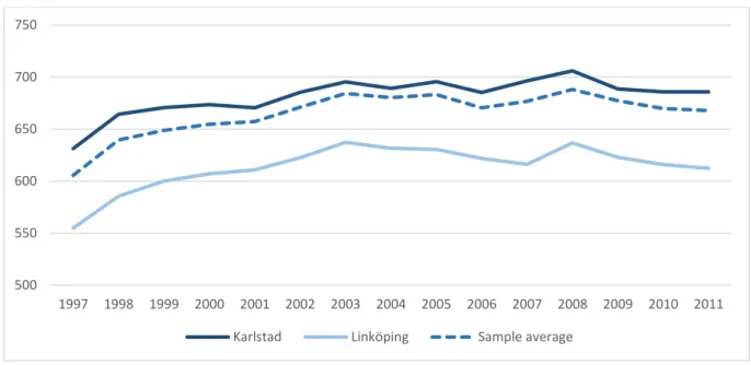
We start by presenting some general information about the municipalities included in the sample and the development of the public transportation system in them. Population growth in the 17 municipalities included in the sample was 10 percent and the growth of private total Vehicle Kilometres Travelled (VKT) was 22 percent over the sample period of 1997-2011. Private VKT per capita grew by 11 percent. We show the development of VKT per capita in two sample municipalities, Linköping, which is the population-wise largest municipality in our sample, and Karlstad, which is one of the smallest municipalities in the sample, in Figure 1. It is obvious from the figure that the growth in private VKT/capita started flattening out at about 2003, reaching a peak in 2008, and declining thereafter.
9
Figure 1. The development of VKT/capita in two sample municipalities, Karlstad (with ca 70 000 inhabitants) and Linköping (with ca 116 000 inhabitants), along with the average for the entire sample.
We have complete public transport data for the entire study period of 1997-2011 for seven out of the seventeen urban areas included in the study.5 The supply of public transport (bus) vehicle
kilometres in these seven urban areas grew by 48 percent. The correlation between the population size and the total private VKT per capita in 2011 was -0.48. The larger a municipality is population-wise, the lower the private VKT per capita. The population growth rate, the change in the total private VKT and private VKT per inhabitant varies across the municipalities in the sample, however. The figures are summarized in Table 1.
Table 1. Variation in population growth, total VKT and VKT/inhabitant growth between 1997 and 2011.
Population Total private VKT
VKT/inhabitant
Average 10 % 22 % 11 %
5 Jönköping, Helsingborg, Lund, Gävle, Karlstad, Landskrona and Trelleborg.
500 550 600 650 700 750 1997 1998 1999 2000 2001 2002 2003 2004 2005 2006 2007 2008 2009 2010 2011 Karlstad Linköping Sample average
10
Max 16 % 38 % 21 %
Min 2 % 13 % 0 %
Looking at year 2011 we see a weaker correlation between the population in the municipality and the supply of bus kilometres per inhabitant 0.37, than the correlation between population in the municipality and the VKT per inhabitant, 0.48. We interpret this as a reflection of the supply of public transport also being determined by other factors, not correlated to population size, as e.g. the share of trips done by cycle or the relative share of the population entitled to free school rides.
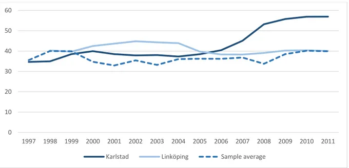
We depict the development of the supply of bus kilometres per capita in Figure 2, the development of trips started per capita in Figure 3, and the number of trips taken per bus kilometre supplied in Figure 4. It is interesting to note the strongly increased supply of bus kilometres per capita in
Karlstad, starting somewhere around 2006 (Figure 2), which results in a corresponding increase in the trips started per capita (Figure 3).
Figure 2. The change in bus kilometres supplied per capita supplied in Karlstad, Linköping and the sample average. 0 10 20 30 40 50 60 1997 1998 1999 2000 2001 2002 2003 2004 2005 2006 2007 2008 2009 2010 2011 Karlstad Linköping Sample average
11
Figure 3. Bus trips started per capita in Karlstad, Linköping and the sample average.
The net effect, however, is to reduce the number of trips started by bus per bus kilometre supplied (Figure 4). For the entire sample, the efficiency of bus kilometre supply in terms of trips started has fallen over the sample period, from about two trips started per bus kilometre supplied to a fairly stable 1.8 trips per bus kilometre (Figure 4).
Figure 4. Bus trips started per supply of bus kilometres in Karlstad, Linköping and the sample average.
0 10 20 30 40 50 60 70 80 90 100 1997 1998 1999 2000 2001 2002 2003 2004 2005 2006 2007 2008 2009 2010 2011 Karlstad Linköping Sample average
0 0,5 1 1,5 2 2,5 1997 1998 1999 2000 2001 2002 2003 2004 2005 2006 2007 2008 2009 2010 2011 Karlstad Linköping Sample average
12
Among the seven urban areas with complete public transport data for the entire period of 1997-2011, the urban area with the highest increase in the production of bus kilometres was in the municipality of Landskrona, where the supply grew by almost 200 percent between 1997 and 2011. In Jönköping, which is one of the population-wise largest municipalities in the sample, the supply of bus kilometres increased only by 5 percent in the sample period. The average increase in bus kilometre supply, excluding Landskrona, was 31 percent. This can be compared to the average population growth in the group of the seven municipalities with complete data of 13 percent. This increase in supply can possibly be explained as a response to the large increase in ridership in these urban areas; the number of started trips grew by 48 percent, even though Figure 4 clearly
demonstrates that the increase in supply has exceeded the increase in demand.
The municipality with the highest population growth in our sample is Lund, which is the fifth largest municipality in the sample. Lund has one of Sweden’s major universities. It is also the municipality with the slowest growth of VKT per capita. The slowest rate of population growth, 2 percent, is in Östersund which is a small municipality in a sparsely populated region in northern Sweden. The private VKT per capita in Östersund increased at the same rate, 11 percent, as the average in the sample. Finally, the fastest growth of VKT per inhabitant, 21 percent, is found in the smallest
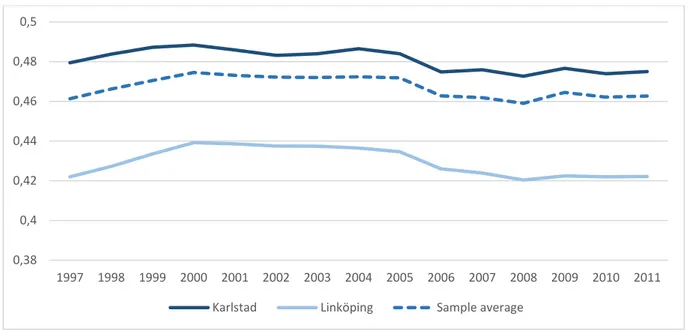
municipality in the sample, Trelleborg. While the development of VKT per capita was shown in Figure 1, we show the development of the share of car owners per capita in Figure 5. It is clear from the figure that car ownership in per capita terms has fallen from the high reached in 2000 - 2005, although not substantially.
13
Figure 5. Share of car owners per capita in Karlstad, Linköping and the sample average.
We drop observations of individuals owning more than 4 cars from the data, altogether 68 177 observations. The reasoning behind this decision is similar to that in Pyddoke and Swärdh (2015), namely that many persons owning more than four vehicles are unlikely to drive all of them by themselves. For example, these cars can be registered on a parent of adult children, e.g., for insurance reasons (the insurance premium is higher for younger persons). Attributing the entire car use to the person formally owning the car might then distort the results. An alternative explanation to owning more than four vehicles is, e.g., that the person collects cars.
The average individual owning more than 4 vehicles is 46.4 years of age. 93.5 percent of them are male. 3 percent are students, 73.6 percent work and 7.9 percent have no job but the tax authorities have information of some work-related taxable income. The rest are unemployed or retired. They have on average 0.85 children and 7.4 cars.
There are some further problems with the car ownership data. It is not possible to identify households in the Swedish register data that we are using. Therefore, the choice of the level of analysis stands between that of an individual, or the entire urban area or municipality. In the present paper, we have decided to use the individual-level data, despite the distortions this creates when the
0,38 0,4 0,42 0,44 0,46 0,48 0,5 1997 1998 1999 2000 2001 2002 2003 2004 2005 2006 2007 2008 2009 2010 2011 Karlstad Linköping Sample average
14
vehicle owned by one member of a household is also used by another member(s), regardless of whether this is a spouse or a child.
Besides information about public transportation, VKT and car ownership, the data also contains information about the individuals residing in the 17 municipalities included in our sample. For 7 377 observations information about the area of the individual’s dwellings is missing, however. We have removed these observations from the data. These individuals vary in age between 18 and 105 years of age, their mean age begin 44.4 years, which is slightly younger than in the sample as a whole (see Table 2). 70.6 percent of them are male. 5.4 percent are students, 11.5 percent work and 8.3 percent have no job but the tax authorities have information of some work-related taxable income. The rest are unemployed or retired. They have on average 0.12 children, varying between 0 and 6 children at most. Their average income in 2011 year’s terms is 70 579 SEK/year over the entire study period, and their average property is 6 626 SEK.6,7 They own between 0 and 47 cars, the average being 1.94 cars
per individual.
Similarly, information about the area of an individual’s work place is missing for 9 329 841 observations. Based on the information in the data, we assume that the individuals in these
observations are either unemployed, retired, self-employed, or students, and have placed their work place in their home, with a commuting distance of 1 metre.8, 9 16.3 percent of the observations in this
group are students, 15.3 percent work and 18.9 percent have no job but the tax authorities have information of some work-related taxable income. The rest are unemployed or retired. The persons are on average 54.6 years old, supporting the assumption of many of them being retirees, the age range varying between 17 and 111 years. They have on average 0.4 children, 46 percent of them are
6 All prices have been deflated using the consumer price index, CPI, from Statistics Sweden.
7 The average exchange rate of the Swedish crown in 2011 was 9.0335 SEK/EUR and 6.4969 SEK/USD. Source: Sveriges Riksbank.
8 We will later on take logarithms of all the variables included in the analysis. In order not to lose the
observations missing information about the location of the work place, we have chosen to set their commuting distance at the shortest possible level. Table 2, showing summary statistics, shows the commuting distance as zero metres for those missing this information, however.
15
male, and they own 0.499 cars varying from 0 to 834. Their average yearly income is 135 099 SEK and the value of the property they own is on average 116 336 SEK.
Several observations in the data have a negative value of disposable income. We have no explanation as to how an individual can have negative disposable income. We have deleted these observations from the data, altogether 46 915 observations. Average disposable income reported in Table 2 includes the negative values, however.
The average individual having a negative income is 40.4 years of age. 50.6 percent of the individuals are male. 8.6 percent have no job but the tax authorities have information of some work-related taxable income, while 78 percent are unemployed. The rest work, are students or retired. The individuals have on average 0.47 children, varying between zero and 9 children. Their mean disposable income is -10 903 SEK.
All the price data (gasoline price, disposable income) is deflated by the consumer price index (CPI) and is expressed in the price terms of 2011. The information about fuel prices is obtained from the Svenska Petroleum & Biodrivmedel Institutet. We use the price of gasoline as a proxy for the fuel price. This is because gasoline driven cars have historically been prevalent in Sweden and because the gasoline and diesel prices are closely correlated. Therefore, including both prices would result in multicollinearity.
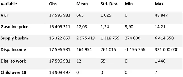
The data used in the regression analyses is summarized in Table 2. The dependent variable is the Vehicle Kilometres Travelled (VKT) in Swedish miles, i.e., tens of kilometres. Gasoline price is a yearly average of the price of gasoline. It obtains the same value for all observations during a given year. Supply bus km is the number of bus kilometres driven within the urban area of a municipality per year. The bus kilometres supplied are divided by the area of the urban area in hectares so that a greater supply of bus kilometres that is due to a large urban area is normalized. The data source for the urban area of a municipality is the same as the source for the bus kilometre data. The variable
16
provides an average measure for the inhabitants relative to the size of the urban area for respective year.
Disp. income is an individual’s disposable income, SEK in 2011 years terms. Dist. to work measures the Euclidian distance between an individual’s home and the work place in kilometres. Child over 18 records the number of children over the age of 18 years residing in an individual’s household. Work takes the value of one if the individual works and zero otherwise. Centre takes a value of 1 if the individual lives within a given distance from the geographical mid-point of the urban area. How big the central area of each municipality is varies from one municipality another depending on an ocular examination of each municipality on a map. Those living in more peripheral areas of the municipality get a zero value on this variable.
Number of cars records the number of cars owned by an individual and varies between zero and 4. Male is an indicator variable taking the value of one for males. Finally, Age is the individual’s age in years, calculated by subtracting from the observation year the individual’s year of birth. In the regression model we use logarithms of all the variables except for: Child over 18, Work, Centre, Number of cars, Male and Age. Moreover, we take first differences of the variables in the regression models, and in some cases, use lagged values.
Table 2. Summary statistics.
Variable Obs Mean Std. Dev. Min Max
VKT 17 596 981 665 1 025 0 48 847 Gasoline price 15 405 311 12,03 1,24 9,90 14,21 Supply buskm 15 322 657 2 975 419 1 318 759 274 000 6 414 550 Disp. Income 17 596 981 164 954 261 015 -1 195 766 331 000 000 Dist. to work 17 596 981 12 55 0 1 446 Child over 18 13 908 497 0 0 0 7
17
Work 17 596 981 0,57 0 0 1
Population density in urban area
15 322 657 21,55 4,52 16,02 40,62
(Domicile in) Centre 17 596 981 0,69 0,46 0 1 Number of cars 1 17 596 981 0,39 0,49 0 1 2 17 596 981 0,063 0,24 0 1 3 17 596 981 0,013 0,11 0 1 4 17 596 981 0,004 0,06 0 1 Male 17 596 981 0,49 0 0 1 Age 17 596 981 47,85 19 17 111
Urban area area ha 15 322 657 3 157 932 1 072 4482
Population 15 322 657 67 311 22 076 24 575 113662 Employment status 5 (unemployed with information about taxable income) 17 596 981 0,12 0,32 0 1 6 (unemployed) 17 596 981 0,31 0,46 0 1
3 The empirical model
The modelling framework is inspired by Dargay (2007). We estimate Vehicle Kilometres Travelled, VKT, by an individual i residing in municipality m at time t. Besides the VKT, the data also contains information about individuals who do not own a car and who consequently do not have any VKT. This feature of the data suggests the use of a selection model, where in the first stage, the participation equation of the probability of an individual owning a car or not is estimated, and in the second stage, conditional on the participation equation, the choice of VKT is estimated. We consider it unadvisable
18
to drop the individuals not owning a car from the data since the supply of public transportation not only influences the VKT but also the decision to own a car. Excluding the non-car owning part of the population would then yield biased estimates of the public transportation’s impact on VKT.
We start by estimating the following participation equation (Greene, 2012, p. 894):
(1) 𝑑𝑖𝑡∗ = 𝒛𝑖𝑚𝑡𝜸 + 𝑢𝑖𝑚𝑡, 𝑢𝑖𝑚𝑡~𝑁[0, 1]
𝑑𝑖𝑡 = 1 if 𝑑𝑖𝑡∗ > 0, 0 otherwise.
𝜸 is the vector of coefficient estimates and 𝒛𝑖𝑚𝑡 consists of variables 𝐶𝑒𝑛𝑡𝑟𝑒𝑖𝑚𝑡, Δ ln(𝐺𝑎𝑠 𝑝𝑟𝑖𝑐𝑒𝑡) Δ ln(𝐵𝑢𝑠 𝑘𝑚𝑚𝑡), Δ ln(𝐵𝑢𝑠 𝑘𝑚𝑚𝑡−1), Δ ln(𝐵𝑢𝑠 𝑘𝑚𝑚𝑡−2), Δ ln(𝐷𝑖𝑠𝑝. 𝑖𝑛𝑐𝑖𝑚𝑡),
Δ ln(𝐷𝑖𝑠𝑡. 𝑡𝑜 𝑤𝑜𝑟𝑘𝑖𝑚𝑡), Δ𝐶ℎ𝑖𝑙𝑑 𝑜𝑣𝑒𝑟 18𝑖𝑚𝑡, Δ𝑊𝑜𝑟𝑘𝑖𝑚𝑡, Δ𝑃𝑜𝑝. 𝑑𝑒𝑛𝑠𝑖𝑡𝑦𝑚𝑡, 𝑀𝑎𝑙𝑒𝑖𝑚𝑡 and 𝐴𝑔𝑒𝑖𝑚𝑡. Δ denotes first differences, i.e., 𝑧𝑖𝑚𝑡− 𝑧𝑖𝑚𝑡−1, and ln 𝑧𝑖𝑚𝑡 is the natural logarithm of variable 𝑧𝑖𝑚𝑡. In some models we also include the interactions of variable 𝐶𝑒𝑛𝑡𝑟𝑒𝑖𝑚𝑡, which indicates whether the individual lives in the urban area or not, with Gasoline price, Disposable income, Distance to work, Child over 18, Work and Population density, in order to capture the difference between the urban and peripheral areas.
After estimating the participation equation, the intensity equation is estimated: (2) 𝑉𝐾𝑇𝑖𝑡∗ = 𝒙𝑖𝑚𝑡′ 𝜷 + 𝜀𝑖𝑚𝑡, 𝜀𝑖𝑚𝑡~𝑁[0, 𝜎2].
𝜷 is the vector of coefficient estimates. 𝒙𝑖𝑚𝑡 consists of the same variables as 𝒛𝑖𝑚𝑡 except that we do not include the twice-lagged Δ ln(𝐵𝑢𝑠 𝑘𝑚𝑚𝑡−2), nor do we include the variables 𝑀𝑎𝑙𝑒𝑖𝑚𝑡 and 𝐴𝑔𝑒𝑖𝑚𝑡 in 𝒙. Moreover 𝒙 also includes Δ ln(𝑁𝑢𝑚𝑏𝑒𝑟 𝑜𝑓 𝑐𝑎𝑟𝑠𝑖𝑚𝑡). Of the centre interactions we include all the ones above, and besides the interactions with Supply bus km (at t and t-1) and the Number of cars. Finally, in most models we also include the predicted, lagged value of the dependent variable, 𝑃𝑟𝑒𝑑𝑖𝑐𝑡𝑒𝑑Δ ln(𝑉𝐾𝑇𝑖𝑚𝑡−1), in 𝒙. Since the inclusion of a lagged dependent variable by construction cause an endogeneity problem, we have, in the first stage, estimated it using the lagged values of the explanatory variables. It is the predicted values that enter the main regression.
19 (3) (a) 𝑉𝐾𝑇𝑖𝑡∗ = 0 if 𝑑
𝑖𝑡 = 0 and 𝑉𝐾𝑇𝑖𝑚 = 𝑉𝐾𝑇𝑖𝑚∗ if 𝑑𝑖𝑡 = 1.
(b) 𝑉𝐾𝑇𝑖𝑡 = 𝑉𝐾𝑇𝑖𝑡∗ if 𝑑𝑖𝑡 = 1 and 𝑉𝐾𝑇𝑖𝑡 is unobserved if 𝑑𝑖𝑡= 0. Finally, the participation and the intensity equations are not uncorrelated of one another:
(4) (𝑢𝑖𝑚𝑡, 𝜀𝑖𝑚𝑡)~bivariate normal with correlation 𝜌. When 𝜌 ≠ 0, standard regression techniques yield biased results.
The motivation for using first-differenced variables is to avoid problems with spurious correlation. Several of the included variables, e.g. VKT, Supply bus km, and Gasoline price, are likely to be following a random walk.10 A first-difference transformation removes the unit root and leads to
stationary variables. Other alternatives, such as a fixed-effect estimator, might also be adequate, but are not used because of the other characteristics of the data.
Since we use a first-difference approach to analyse the dependent variable 𝑉𝐾𝑇𝑖𝑚𝑡 by estimating the dynamic panel data model, it is not possible to include time-invariant variables like the gender or birth year in the analysis. At the same time, the individual-specific effect 𝜇𝑖 is cancelled out. The functional form is a log-log specification, which implies that the parameters of the continuous variables can be interpreted as elasticities. The parameter estimates of the indicator variables, most notably Child over 18, Work and Centre can be transformed into percentage changes by the formula 𝑒𝑥𝑝(𝛽𝑥) − 1. The functional form implies constant elasticity over the 17 municipalities studied and over time, income quantiles etc.
We estimate the model in equations (1) to (4) using the Heckman selection model using a maximum likelihood estimation procedure. We run the model using Stata’s vce(robust) command.
As Greene (2012, p. 915) notes, the marginal effect of any explanatory variable on 𝑉𝐾𝑇𝑖𝑚𝑡 in the observed sample consists of two components. The direct effect on the mean of 𝑉𝐾𝑇𝑖𝑚𝑡 is measured
10 Without any further information, the best prediction of the value of the variable in time t+1 is the value of the variable in time t.
20
by 𝜷. In addition, an independent variable that also appears in the probability that 𝑑𝑖∗ is positive influences 𝑉𝐾𝑇𝑖𝑚𝑡 through its presence in 𝜆𝑖. The full effect of changes in an explanatory variable that appears both in the main and in the selection model is
(5) 𝜕𝐸[𝑉𝐾𝑇𝑖𝑚𝑡|𝑑𝑖∗> 0] 𝜕𝑥𝑖𝑚𝑡𝑘 = 𝛽𝑘− 𝛾𝑘( 𝜌𝜎𝜖 𝜎𝑢 ) 𝛿𝑖(𝛼𝑢),
where 𝛿𝑖 = 𝜆𝑖2− 𝛼𝑖𝜆𝑖, 𝛼𝑢= − 𝒛𝑖𝑚𝑡′ 𝜸 𝜎⁄ 𝑢 and 𝜆(𝛼𝑢) = 𝜙(𝒛𝑖𝑚𝑡′ 𝜸/𝜎𝑢) Φ(𝒛⁄ 𝑖𝑚𝑡′ 𝜸 𝜎⁄ 𝑢), the inverse Mills ratio. Moreover, 𝜎𝑢~𝑁(0,1).
4 Regression results
Table 3 shows results from four model estimations. In column (1) we completely exclude the lagged dependent variable, Δ𝑙𝑛(𝑉𝐾𝑇𝑡−1). In the other models we first estimate the first-differenced lagged dependent variable in a first-stage model, using a Heckman selection model even at this stage but excluding the lagged ln(VKT) from the estimation (using in effect a model similar to that shown in column (1) but once lagged), and use the predicted values to estimate the main models shown in columns (2) to (4). In the model of column (3) we also include the interaction terms of the explanatory variables with an indicator variable for the individual living in the urban area
(𝐶𝑒𝑛𝑡𝑟𝑒𝑖𝑚𝑡). In column (4) we have excluded most of the insignificant centre interactions from the model. The variable names in Table 3 differ somewhat from the above; above all, we have left out Δ, “ln”, and the individual, municipality and time subscripts out of the notation, indicating once lagged values of variables with “lag” and twice lagged values with “lag2” instead. Interactions are denoted by #, and apply for 𝐶𝑒𝑛𝑡𝑟𝑒𝑡= 1.
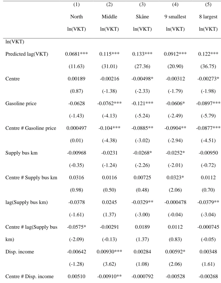
Table 3. Results from a Heckman selection model using a maximum likelihood estimation procedure.
(1)
(2)
(3)
(4)
ln(VKT)
ln(VKT)
ln(VKT)
ln(VKT)
21
Predicted lag(VKT)
0.111***
0.111***
0.111***
(42.25)
(42.10)
(42.10)
Centre
-0.00333**
-0.00314**
(-3.13)
(-3.06)
Gasoline price
-0.122***
-0.123***
-0.0802***
-0.0801***
(-15.16)
(-15.34)
(-6.19)
(-6.18)
Centre # Gasoline price
-0.0957***
-0.0959***
(-5.87)
(-5.89)
Supply bus km
-0.00187
-0.00240
-0.0173
-0.0182*
(-0.35)
(-0.45)
(-1.92)
(-2.05)
Centre # Supply bus km
0.0201
0.0215*
(1.81)
(1.97)
lag(Supply bus km)
-0.0112*
-0.0117*
-0.0163*
-0.0162*
(-2.36)
(-2.45)
(-2.03)
(-2.02)
Centre # lag(Supply bus
km)
0.00248
0.00242
(0.25)
(0.24)
Disp. income
0.00254*
0.00224*
0.00461**
0.00475**
(2.50)
(2.18)
(2.64)
(2.74)
Centre # Disp. income
-0.00390
-0.00413
(-1.81)
(-1.93)
Dist. to work
0.00672***
0.00681***
0.00679***
0.00679***
(14.32)
(14.53)
(8.92)
(14.49)
Centre # Dist. to work
-0.0000431
(-0.04)
22
(9.06)
(8.60)
(6.40)
(8.62)
Centre # Child over 18
-0.00297
(-1.09)
Work
0.00961***
0.00971***
0.0115***
0.00948***
(5.26)
(5.31)
(3.77)
(5.18)
Centre # Work
-0.00320
(-0.84)
Population density
0.0318
0.0277
-0.0265
-0.00119
(1.14)
(0.99)
(-0.50)
(-0.04)
Centre # Population density
0.0360
(0.58)
Number of cars
0.436***
0.447***
0.412***
0.412***
(290.62)
(293.15)
(192.35)
(192.39)
Centre # Number of cars
0.0685***
0.0684***
(22.84)
(22.83)
select
Centre
-0.520***
-0.520***
(-448.68)
(-448.69)
Gasoline price
-1.198***
-1.199***
-1.868***
-1.868***
(-115.42)
(-115.44)
(-101.50)
(-101.50)
Centre # Gasoline price
1.533***
1.533***
(68.55)
(68.55)
Supply bus km
-0.272***
-0.273***
-0.172***
-0.172***
(-39.13)
(-39.22)
(-24.57)
(-24.57)
23
(-47.37)
(-47.45)
(-26.87)
(-26.87)
lag2(Supply bus km)
-0.335***
-0.335***
-0.171***
-0.171***
(-52.48)
(-52.51)
(-26.76)
(-26.76)
Disp. income
-0.0187***
-0.0193***
-0.0242***
-0.0242***
(-23.10)
(-23.74)
(-13.65)
(-13.65)
Centre # Disp. income
0.0131***
0.0131***
(6.61)
(6.61)
Dist. to work
0.000649
0.000637
-0.0108***
-0.0108***
(1.11)
(1.09)
(-9.91)
(-9.91)
Centre # Dist. to work
0.0126***
0.0126***
(9.72)
(9.72)
Child over 18
-0.0104***
-0.0103***
-0.00900**
-0.00901**
(-5.18)
(-5.14)
(-2.75)
(-2.75)
Centre # Child over 18
0.00991*
0.00992*
(2.35)
(2.35)
Work
-0.166***
-0.166***
-0.0706***
-0.0706***
(-80.70)
(-80.76)
(-17.23)
(-17.23)
Centre # Work
-0.0942***
-0.0941***
(-19.92)
(-19.92)
Population density
-1.080***
-1.080***
-2.120***
-2.120***
(-38.77)
(-38.77)
(-25.93)
(-25.93)
Centre # Population density
1.451***
1.451***
(16.92)
(16.92)
Male
0.640***
0.640***
0.726***
0.726***
24
Age
-0.00723***
-0.00724***
-0.00203***
-0.00203***
(-560.72)
(-561.14)
(-114.85)
(-114.87)
athrho
Constant
0.00125
-0.00408***
0.00349*
0.00324*
(1.47)
(-4.79)
(2.19)
(2.10)
lnsigma
Constant
-0.467***
-0.467***
-0.467***
-0.467***
(-366.70)
(-366.97)
(-366.96)
(-366.96)
Observations
6723656
6721437
6721437
6721437
AIC
14273210.4
14262093.4
14017245.3
14017239.9
BIC
14273512.3
14262408.9
14017794.1
14017733.8
t statistics in parentheses * p<0.05, ** p<0.01, *** p<0.001Based on the Akaike information criterion (AIC), the model in column (4) is our preferred model. According to this criterion, the model in column (3) is 0.067 times as probable as the model in column (4) to minimize the information loss. The models in columns (1) and (2) are not at all likely to minimize the information loss compared to the model in column (4), the relative probability of their AIC measures being zero at least at a 20 decimal level compared to model (4).
The Wald test of independent equations indicates that in model (1), 𝜌 = 0 cannot be rejected at a conventional level of statistical confidence. In this case the standard estimation technique does not yield biased estimates of the coefficients. For the models in columns (2) to (4) the Wald test yields a significant 𝜒2 test value, however. Consequently, we cannot assume that a standard estimation technique would yield unbiased coefficient estimates.
25
We calculate both the short-term and the long-term elasticity of VKT to the supply of bus kilometres. The long-term elasticity refers to the time when all adjustments are made. Literally, we will never reach the new equilibrium as there will always be a (negligible) small part left of the persistence of VKT. In practice, however, the lagged dependent variable of 0.111 in Table 3 implies that about 89 percent of the adjustment to the new equilibrium is made already during the first year. Then 89 percent of the remaining persistence is adjusted during the second year. This implies that 89 + 89×0.11, almost 99 percent of the adjustment is made after 2 years.
The parameters used to calculate the marginal effects from equation (5) are obtained in conjunction with the estimation procedure. The shortterm elasticity of VKT to the supply of bus kilometres is -0.034 in the peripheral and -0.0098 in the urban areas. This was calculated adding together the coefficients for all the lags of the variable Supply bus kilometres in the selection equation. The long-term elasticity of VKT to the supply of bus kilometres is -0.038 in the peripheral areas and -0.011 in the urban area. The difference between the elasticities for outside and inside an urban area is quite considerable. Both the short-term and the long-term elasticities are very low in the municipalities in the sample. These results are summarized in the second column of Table 5.
In order to check the robustness of our model vis-à-vis previous studies, we even calculate the fuel price elasticities implicit in the results in Table 3. The short term fuel price elasticity is -0.078 and the long-term elasticity is -0.087. These elasticities do not apply for those living in the urban area,
however, as is indicated by the significant coefficient on the interaction between Centre and Gasoline price. The short-term fuel price elasticity for the residents in the urban area is -0.176 and the long-term elasticity is -0.197, much higher than the elasticity for those living outside the centre. The estimated fuel price elasticities in the urban area fall fairly well in line with those found in Graham and Glaister (2002), who estimate the short term elasticity of 0.16, and the long term elasticity of -0.26, and Dargay (2007), who estimate the short term elasticity of -0.10 and the long term elasticity of -0.14 but are lower than those found in Pyddoke and Swärdh (2015). While Pyddoke and Swärdh’s
26
main estimates are differentiated by gender, geography and income, their average estimate of fuel price elasticities for the urban areas is a shortterm elasticity of 0.25 and a longterm elasticity of -0.45.
Other coefficients of interest arise from the ‘select’ equation only. Thus, a 1 percent increase in the population density of the urban area lowers car ownership by 2.12 percent in the peripheral areas. In the urban area, a 1 percent increase in population density lowers car ownership less, only by 0.67 percent. A 1 percent increase in the gasoline price lowers car ownership by 1.87 percent in the peripheral areas and by 0.34 percent in the urban area.
As a robustness test we ran the results in column (4) of Table 2 also using the Heckman two-stage estimator. The coefficient estimates are very close to the ones obtained using maximum likelihood, i.e. the estimates in column 4 in Table 3. There are some differences in the standard errors, however. The largest difference is in the interaction variable Centre # Disp. income, which has a significant coefficient of the same size as that reported in column (4), in the two-stage regression. Otherwise the results do not change in a statistically significant manner.
As an additional robustness check, we clustered the data according to the municipality’s geographical location: north (Gävle, Luleå, Sundsvall and Östersund), middle Sweden (Borås, Halmstad, Jönköping, Karlstad, Linköping, Norrköping, Skövde and Växjö) and Skåne (Helsingborg, Kristiandstad,
Landskrona, Lund and Trelleborg). We also clustered the data by population size, grouping the 9 by population smallest municipalities in one cluster and the 8 largest municipalities in another. We estimate a model similar to the one in column (4) of Table 2 separately for each of these five clusters. The results for the regional division model are shown in columns (1) to (3) of Table 4. The results from the model dividing the data according to the municipalities’ population are shown in columns (4) and (5).
27
Table 4. Results from a Heckman selection model, for data divided according to geographic location of the municipality respectively municipality’s population size. Estimated using maximum likelihood.
(1)
(2)
(3)
(4)
(5)
North
Middle
Skåne
9 smallest
8 largest
ln(VKT)
ln(VKT)
ln(VKT)
ln(VKT)
ln(VKT)
ln(VKT)
Predicted lag(VKT)
0.0681***
0.115***
0.133***
0.0912***
0.122***
(11.63)
(31.01)
(27.36)
(20.90)
(36.75)
Centre
0.00189
-0.00216
-0.00498*
-0.00312
-0.00273*
(0.87)
(-1.38)
(-2.33)
(-1.79)
(-1.98)
Gasoline price
-0.0628
-0.0762***
-0.121***
-0.0606*
-0.0897***
(-1.43)
(-4.13)
(-5.24)
(-2.49)
(-5.79)
Centre # Gasoline price
0.000497
-0.104***
-0.0885**
-0.0904**
-0.0877***
(0.01)
(-4.38)
(-3.02)
(-2.94)
(-4.51)
Supply bus km
-0.00968
-0.0231
-0.0268*
-0.0252*
-0.00950
(-0.35)
(-1.24)
(-2.26)
(-2.01)
(-0.72)
Centre # Supply bus km
0.0316
0.0116
0.00725
0.0323*
0.0112
(0.98)
(0.50)
(0.48)
(2.06)
(0.70)
lag(Supply bus km)
-0.0378
0.0245
-0.0329**
-0.000478
-0.0379**
(-1.61)
(1.37)
(-3.00)
(-0.04)
(-3.04)
Centre # lag(Supply bus
km)
-0.0575*
-0.00291
0.0189
0.0112
-0.000745
(-2.09)
(-0.13)
(1.37)
(0.83)
(-0.05)
Disp. income
-0.00642
0.00930***
0.00284
0.00592*
0.00348
(-1.28)
(3.62)
(1.08)
(2.06)
(1.61)
28
(0.88)
(-2.86)
(-0.24)
(-1.44)
(-1.02)
Dist. to work
0.00628***
0.00633***
0.00764***
0.00672***
0.00679***
(6.26)
(9.26)
(9.11)
(8.57)
(11.61)
Child over 18
0.0127***
0.0135***
0.00724**
0.0126***
0.0109***
(4.14)
(7.14)
(2.98)
(5.64)
(6.52)
Work
0.00257
0.00963***
0.0149***
0.00823**
0.0104***
(0.65)
(3.63)
(4.52)
(2.69)
(4.58)
Population density
-0.230
0.154
-0.148*
-0.119
0.0926
(-0.93)
(1.75)
(-2.13)
(-1.73)
(1.12)
Centre # Pop. density
0.301
-0.244*
0.226**
0.0317
-0.0501
(1.12)
(-2.35)
(2.72)
(0.38)
(-0.53)
Number of cars
0.409***
0.446***
0.478***
0.436***
0.453***
(120.02)
(209.69)
(169.11)
(176.63)
(233.87)
select
Centre
-0.424***
-0.522***
-0.592***
-0.448***
-0.557***
(-167.46)
(-296.39)
(-287.41)
(-226.93)
(-356.64)
Gasoline price
-2.036***
-2.020***
-1.678***
-1.994***
-1.786***
(-39.02)
(-78.41)
(-52.75)
(-58.90)
(-81.02)
Centre # Gasoline price
1.717***
1.776***
1.224***
1.450***
1.498***
(30.32)
(55.38)
(32.27)
(34.75)
(56.36)
Supply bus km
-0.290***
0.0206
-0.0553***
-0.158***
-0.222***
(-16.04)
(1.51)
(-5.57)
(-15.67)
(-22.28)
lag(Supply bus km)
0.0519**
0.0476***
-0.297***
-0.126***
-0.212***
(3.13)
(3.69)
(-33.42)
(-14.32)
(-23.81)
lag2(Supply bus km)
0.00144
-0.0314*
-0.208***
-0.0846***
-0.264***
29
(0.09)
(-2.13)
(-25.13)
(-9.41)
(-28.78)
Disp. income
-0.0248***
-0.0291***
-0.0185***
-0.0206***
-0.0256***
(-5.20)
(-10.82)
(-6.87)
(-7.19)
(-11.40)
Centre # Disp. income
0.00884
0.0131***
0.0139***
0.00751*
0.0156***
(1.67)
(4.33)
(4.68)
(2.27)
(6.32)
Dist. to work
-0.00680**
-0.0112***
-0.0113***
-0.0139***
-0.00797***
(-2.69)
(-7.24)
(-5.84)
(-7.89)
(-5.71)
Centre # Dist. to work
0.00961**
0.0149***
0.00991***
0.0152***
0.00989***
(3.29)
(7.96)
(4.32)
(7.09)
(6.05)
Child over 18
-0.00984
-0.00684
-0.0120*
-0.00652
-0.0101*
(-1.16)
(-1.53)
(-2.05)
(-1.20)
(-2.46)
Centre # Child over 18
0.0175
0.00360
0.0163*
0.00383
0.0129*
(1.72)
(0.61)
(2.14)
(0.54)
(2.45)
Work
-0.0679***
-0.0727***
-0.0710***
-0.0624***
-0.0765***
(-7.02)
(-12.47)
(-9.89)
(-9.39)
(-14.68)
Centre # Work
-0.0686***
-0.106***
-0.0896***
-0.0993***
-0.0883***
(-6.28)
(-15.60)
(-10.84)
(-12.60)
(-14.88)
Population density
-0.861***
-3.075***
-1.850***
-0.369***
-4.754***
(-3.68)
(-19.32)
(-18.22)
(-4.40)
(-25.82)
Centre # Pop. density
2.347***
3.233***
0.376***
1.370***
3.429***
(9.62)
(19.78)
(3.43)
(14.52)
(18.35)
Male
0.799***
0.744***
0.652***
0.732***
0.726***
(367.79)
(533.47)
(376.52)
(442.23)
(602.64)
Age
-0.00306*** -0.00222*** -0.00113*** -0.00228*** -0.00177***
30
Athrho
Constant
-0.0111**
0.00306
0.00989***
-0.00187
0.00506*
(-3.14)
(1.32)
(3.31)
(-0.71)
(2.46)
Lnsigma
Constant
-0.467***
-0.467***
-0.469***
-0.461***
-0.471***
(-157.65)
(-261.25)
(-205.39)
(-221.56)
(-292.56)
Observations
1347671
3276438
2097328
2289017
4432420
AIC
2857677.8
6858849.2
4285312.8
4907672.3
9101919.5
BIC
2858113.9
6859317.3
4285764.8
4908127.5
9102398.4
t statistics in parentheses * p<0.05, ** p<0.01, *** p<0.001The Wald test of independent equations indicates that in models (1), (3) and (5), 𝜌 ≠ 0 at a conventional level of statistical significance. We conclude that the Heckman specification is the correct one.
The differences in the coefficient estimates for the three regions in columns (1) to (3) are quite considerable. We calculate the total effect using equation (5). The elasticity of VKT to bus kilometre supply in the central (peripheral) areas in the municipalities in the north of Sweden is -0.068 (-0.073) in the short run, and -0.073 (-0.078) in the long run. In the mid-Sweden, the elasticity is 0.0086 (0.0073) in the short run and 0.0098 (0.0083) in the long run. This would seem to indicate that increased supply of public transport in this area actually raises the VKT. Since the coefficients on Supply bus km in the main model of column 2 are all insignificant, we conclude that the effect is in fact zero. In Skåne in the southernmost Sweden the elasticity of VKT to bus kilometres supplied in the central (peripheral) areas is again negative at -0.029 (-0.061) in the short term and -0.034 (-0.070) in the long run. We conclude that the elasticity of VKT to the bus kilometres supplied in the entire country is very low. The marginal effects are summarized in the last three columns of Table 5.
31
The estimates also vary quite a lot between the population-wise small and the larger municipalities (columns (4) and (5) of Table 4). The elasticity of VKT to the bus kilometres supplied in the central (peripheral) areas of the smaller municipalities is 0.018 (-0.027) in the short run and 0.020 (-0.029) in the long term. This can be compared to elasticities of -0.035 (-0.043) in the short run and -0.040 (-0.050) in the long run in the larger municipalities. An increase in the supply of public transportation thus has many times greater impact in reducing the VKT in the larger municipalities than in the small ones. The results are summarized in the third and fourth columns of Table 5
Table 5. Summary of the estimated marginal effects. Blanks indicate insignificant parameter estimates.
General 9 smallest 8 largest North Middle Skåne Short term - urban -0.0098 -0.035 -0.068 -0.029 Short term - periphery -0.034 -0.027 -0.043 -0.073 -0.061 Long term - urban -0.011 -0.04 -0.073 -0.034 Long term - periphery -0.038 -0.029 -0.05 -0.078 -0.07
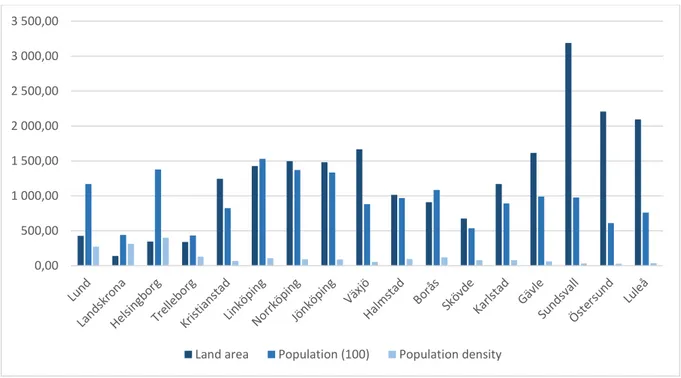
An explanation to the regional differences is in place. Four out of the five area-wise largest municipalities in the sample lie in the north of Sweden, the exception being Växjö, which has a greater land area than Gävle. While the municipalities in the north of Sweden may population-wise be larger than municipalities further to the south, four out of the five municipalities with the lowest
32
population density also lie in the north of Sweden, the exception again being Växjö, which has a lower population density than Gävle. This information is shown in Figure 6.
The north of Sweden is therefore relatively sparsely populated, with low population densities. Raising the supply of bus kilometres would probably increase ridership and consequently lower the private VKT travelled. Whether it is economically feasible to increase the supply of bus kilometres in this manner is questionable, however, due to the low population density of these areas. The low
elasticity of VKT to the gasoline price reflects the flip side of the coin: since the public transportation network is thin, the elasticity of car use is low. There are no alternatives to car in this region.
Figure 6. Land area, population (in 100 persons) and population density in the sample municipalities. The five left-most municipalities lie in Skåne, the next eight are in middle Sweden and the four right-most are in the north of Sweden.
The results in mid-Sweden were for us unexpected. The municipalities in this area have a fairly large area and relatively high populations. Their public transport systems are probably quite well
0,00 500,00 1 000,00 1 500,00 2 000,00 2 500,00 3 000,00 3 500,00
33
developed. It may then be unfeasible to reduce car-ridership by increasing the supply of public transportation.
The municipalities in the Skåne region are quite small area-wise, the exception being Kristianstad. These municipalities also have the highest population density of the municipalities included in our sample, Kristianstad again being the exception. Their absolute population varies between the second-largest in the sample, Helsingborg, and the smallest in the sample, Trelleborg. We assume that the responsivity of the municipalities in Skåne to an increase in the supply of public
transportation is due to their relatively high population densities. The gasoline price elasticity is also highest in Skåne, indicating the availability of alternatives to driving a car.
5 Conclusions
The purpose of this study has been to produce empirical estimates of the elasticity of Vehicle
Kilometres Travelled (VKT) to the supply of public transportation in Sweden using administrative data on private individual car ownership and car use. We have analysed 17 mid-sized Swedish
municipalities, including information about the bus kilometres supplied in their urban areas, as a measure of the public transportation supply. This measure captures the main part of the public transportation supply within the urban areas of these municipalities. Only in Norrköping is the bus system complemented by trams within the urban area. Commuter trains typically serve commuting between municipalities.
An important feature of the present study is the inclusion of the entire adult population in the 17 municipalities in the study. Thus, we have not only studied the impact of public transportation supply on the driving behaviour of car-owners, but on the entire population, that is, on the decision to own a car or not. This gives us results for the total impact of changes in public transportation supply, including changes in car ownership. It has also allowed us to estimate the total fuel price elasticity of private VKT, not only a measure restricted to the car-owning population. This gives valuable
34
supply of public transport, and also in fuel prices and taxation, and the chances of reducing car-driving and the associated emissions using economic policy instruments (taxes).
Availability of public transportation data restricts our sample to the 17 municipalities. Future data availability allowing, it remains to exploit the data set, which contains individual information about all adult residents of Sweden for the period from 1997 to 2011, for future more comprehensive studies of public transportation supply’s possibilities to reduce car driving in Sweden.
Our main result is that the supply of bus kilometres in mid-sized Swedish municipalities reduces vehicle kilometres travelled. The impact is, however, very small. Previous studies suggest that congestion and costs associated with obtaining parking may be the main causes for reduced private car use in cities. These are not likely to be important factors in mid-sized municipalities with little congestion and ample parking space.
A 1 percent increase in the bus kilometres supplied in our sample only reduces private VKT by 0.0098 - 0.034 per cent in the short run. In the long term the impact is greater, the reduction being between 0.011 and 0.038 percent depending on whether we study the central or the peripheral areas of the municipalities. Interestingly, the private VKT is more elastic vis-à-vis the bus kilometres supplied in the peripheral areas of the municipalities than in the urban area. A possible explanation for this may be that inhabitants in the urban part of a municipality may be more likely to choose walking or cycling as alternatives to private car use. Unfortunately we do not have data on cycling in order to study the question further.
These average results mask quite considerable differences between municipalities of different population sizes, however. Thus, the 9 smallest municipalities have an elasticity of private VKT to bus kilometres supplied that is, in effect, zero in the urban parts of the municipalities. In the largest 8 municipalities a 1 percent increase in the bus kilometres supplied reduces private VKT by an estimated 0.035 to 0.043 per cent in the short run. The differences between the different parts of Sweden, the north, middle and Skåne, are quite considerable, too.
35
Finally, these results show that the hypothesis that the increase in public transport is the main cause for the stagnating increase of total private VKT per inhabitant in the sample municipalities is probably not true. It therefore remains for future research to explain the causes behind this phenomenon.
References
Adler, M. W., & van Ommeren, J. (2015). Does public transit reduce car travel externalities? Quasi-natural experiments' evidence from transit strikes. Amsterdam: Working Paper, VU University of Amsterdam.
Anderson, M. (2014). Subways, strikes, and slowdowns: The impacts of public transit on traffic congestion. American Economic Review, 104(9), 2763-2796.
Beaudoin, J., Farzin, Y. H., & Lawell, C. (2015). Public transit investment and sustainable
transportation: A review of studies of transit's impact on traffic congestion and air quality. Research in Transportation Economics, 52, 15-22.
Brownstone, D., & Golob, T. (2009). The impact of residential density on vehicle usage and energy consumption. Journal of Urban Economics, 65, 91-98.
Cervero, R., & Murakami, J. (2010). Effects of built environments on vehicle miles traveled: evidence from 370 US urbanized areas. Environment and Planning, 42, 400-418.
Dargay, J. (2007). The effect of prices and income on car travel in the UK. Transportation Research Part A, 41, 949.-960.
Duranton, G., & Turner, M. (2011). The fundamental law of road congestion: Evidence from US cities. American Economic Review, 101, 2616-2652.
Echenique, M., Hargreaves, A., Mitchell, G., & Namdeo, A. (2012). Growing cities sustainably. Journal of the American Planning Association, 78, 121-137.
36
Glaser, E., & Kahn. (2010). The greenness of cities: Carbon dioxide emissions and urban development. Journal of Urban Economics, 67, 404-418.
Graham, D., & Glaister, S. (2002). Review of income and price elasticities of demand for road traffic. Centre for Transport Studies, Imperial College of Science.
Greene, W. H. (2012). Econometric Analysis (7th ed.). Boston: Prentice Hall.
McIntosch, J., Trubka, R., Kenworthy, J., & Newman, P. (2014). The role of urban form and transit in city car dependence: Analysis of 26 globali cities from 1960 to 2000. Transportation Research Part D, 33, 95-110.
Norheim, B. (2006). Kollektivtransport i nordiske byer - markedspotential og utfordringer framover. Urbanet 2/2006.
Pyddoke, R., & Swärdh, J.-E. (2015). Differences in the effects of fuel price and income on private car use in Sweden 1999-2008. CTS Working Paper 2015:1.