An Exploratory Comparison of B-RAAM and RAAM Architectures

(1)

architectures (HS-IDA-EA-03-302)

Andreas Kjellberg (a99andkj@ida.his.se)

Department of Computer Science University of Skövde, Box 408

S-54128 Skövde, SWEDEN

Dissertation for the degree of M.Sc., in the department of Computer Science Spring 2003.

(2)

architectures

Submitted by Andreas Kjellberg to Högskolan Skövde as a dissertation for the degree of M.Sc., in the Department of Computer Science.

[2003-06-13]

I certify that all material in this dissertation which is not my own work has been identified and that no material is included for which a degree has previously been conferred on me.

Signed: _______________________________________________

(3)

Artificial intelligence is a broad research area and there are many different reasons why it is interesting to study artificial intelligence. One of the main reasons is to understand how information might be represented in the human brain. The Recursive Auto Associative Memory (RAAM) is a connectionist architecture that with some success has been used for that purpose since it develops compact distributed representations for compositional structures.

A lot of extensions to the RAAM architecture have been developed through the years in order to improve the performance of RAAM; Bi coded RAAM (B-RAAM) is one of those extensions. In this work a modified B-RAAM architecture is tested and compared to RAAM regarding: Training speed, ability to learn with smaller internal representations and generalization ability. The internal representations of the two network models are also analyzed and compared. This dissertation also includes a discussion of some theoretical aspects of B-RAAM.

It is found here that the training speed for B-RAAM is considerably lower than RAAM, on the other hand, RAAM learns better with smaller internal representations and is better at generalize than B-RAAM. It is also shown that the extracted internal representation of RAAM reveals more structural information than it does for B-RAAM. This has been shown by hieratically cluster the internal representation and analyse the tree structure. In addition to this a discussion is added about the justifiability to label B-RAAM as an extension to RAAM.

Keywords: Artificial intelligence, Bi coded RAAM, RAAM, B-RAAM and

(4)

I want thank my supervisor Henrik Jacobsson for excellent supervising and for always pushing me in the right direction throughout the project.

I also want to thank Andreas Hansson for let my use the RAAM and B-RAAM implementation, and for all the help and counselling.

Thanks to Maria for keep boosting my confidence and for sending so much positive energy, despite the distance. Hopefully I will get the chance to pay you back.

(5)

1. Introduction

Artificial intelligence is a broad research area and there are many different reasons why it is interesting to study artificial intelligence. One of the main reasons is to understand how information might be represented in the human brain. There are two main schools debating how the human mind is best modelled. These schools are

connectionists and classicists. In the late 80’s and in the 90’s this debate occupied a

number of researchers in the field of artificial intelligence.

Fodor and Pylyshyn's often cited paper (1988) launches the debate of lack of

systematicity in the connectionists’ model. The systematicity of language refers to the

fact that the ability to produce/understand/think some sentences is intrinsically connected to the ability to produce/understand/think others of related structure. Fodor and Pylyshyn (1988) point out that the ability for humans to entertain one thought implies the ability to entertain thoughts with semantically related contents. If we can think ‘John loves the girl’ we also, according to Fodor & Pylyshin, must be able to think ‘the girl loves John’. Also if we can infer ‘John went to the store’ from John and Bob and Sue went to the store’ we must be able to infer ‘John went to the store’ from ‘John and Bob and Sue and Jim went to the store’.

The basic condition for systematicity is compositionality. Representations may be said to be compositional insofar as they retain the same meaning across diverse contexts. Thus, "kick" means the same thing in the context of "-the ball", "- a rock",

and "- a dog", although it changes meaning in the context of "- the bucket"1. One

might say that according to the principle of the compositionality of representations atomic representations make the same semantic contribution in every context in which they occur. The lack of compositionality was the main criticism against connectionism. Fodor & Pylyshin state that a connectionist network consists of a number of interconnected nodes that are only causally related to each other, and there are no structural relations, as in the classical model. According to the classicists, compositionality is easy to accomplish in the classical model, just concatenate the constituents into a complex representation.

Pollack (1990) made a great impact on the systematicity debate when he introduced the RAAM architecture, presented later in this dissertation. The RAAM architecture provided the connectionists with mechanisms for compositionality and systematicity. Chalmers (1990) used the RAAM architecture in combination with a feed-forward network to show that connectionist architectures can represent more complex structures and make spatially sensitive processes possible; the network can model syntactic transformations on a represented sequence, e.g. ‘John Love Mary’ could be transformed into ‘Mary is Loved By John’. Chrisman (1991) used a Dual-ported RAAM to merge representation and processing. According to Chrisman, representation for a sequence can support the processing of it. Niklasson and Sharkey (1992) trained the RAAM architecture to separate complex and atomic representations. In the conclusion of their article they state that in the extended RAAM architecture they used, compositionality and systematicity could be achieved. “We have shown that connectionism can accomplish compositionality and systematicity. The

(7)

superpositional representations with non-classical constituents.” (Niklasson and Sharkey, 1993, p. 12).

Since Pollack (1990) introduced the RAAM architecture, a number of variations and extensions of the architecture have been developed, e.g. Extended RAAM (Niklasson & Sharkey, 1992), Two Layer Digital RAAM (Blair, 1995), Recursive

Hetero-Associative RAAM (Forcada and Ñeco, 1997), Dual Ported RAAM Chrisman,

1990 and Infinite RAAM (Levy, S., Melnik, O. and Pollack, J.B. (2000).

Adamson and Damper (1999) developed Bi Coded RAAM (B-RAAM) which is yet another variation of RAAM. The first change they introduced was a delay-line where the representations of previously decoded sequences where re-fed into the current representation. The second change was that the entire sequence was decoded simultaneously. An extensive description of B-RAAM will be given in chapter 2.3.

The purpose of this dissertation is to investigate and evaluate the Bi Coded RAAM in order to see if it has all the properties stated by its originators Adamson & Damper (1999). By replicating some experiments earlier conducted on RAAM by Blank, Meeden, L. & Marshall, J. (1991), Bi Coded RAAM and RAAM will be compared.

1.1 Motivation

There exist a lot of different RAAM extensions, all with different deviations from the original architecture. So why study Bi Coded RAAM? As its originators (Adamson & Damper 1999) states, Bi Coded RAAM undeniably has some appealing advantages over RAAM. Its ability to converge in fewer training epochs and its ability to cope with noise in input makes it an interesting architecture to take a closer look at.

Depending on the area of research there are different reasons to study RAAM. For example there is some research on different RAAM architectures and their ability to model human sequence representation and processing (cf. Hansson and Niklasson (2001); Hansson and Niklasson (2002)). Callan (1999) mentions several reasons why it is interesting to study RAAM. As already stated it has been used as an argument for connectionists in the refutation of the earlier criticism that connectionist architectures lack compositionality and systematicity. Callan (1999) also point out that “RAAM has caught the imagination of the connectionist community and there is a growing base of research and literature.” (Callen, 1999, p. 175). Finally Callen (1999) state that the most important reason is that it is a useful architecture for exploring some of the key issues concerning representation.

Although this dissertation does not focus on what RAAM can be used for, it will focus on evaluating the Bi Coded RAAM architecture by comparing it to its predecessor.

Bi Coded RAAM seems to be a promising architecture. As Hansson & Niklasson (2001) points out, the previously encoded parts of the sequence are fed back into the current representation and increase the influence of the earlier input. They also point out that the entire sequence is decoded simultaneously, allowing the output to grow dynamically with the sequence, whereas in RAAM, the size of the output is fixed.

B-RAAM is chosen to be investigated because it seems to make less error when decoding sequences and training seems be less time consuming in comparison to RAAM. According to Hansson & Niklasson (2001) B-RAAM also have the potential to model some of the constraints in human short and long term memory.

(8)

2. Background

This chapter will present the basic ideas and concepts behind this dissertation. In Section 2.1 the most basic ideas behind distributed representation of knowledge will be presented, artificial neural networks and a simple neuron will be explained; further a short description of recurrent networks will be presented. In Section 2.2 the RAAM architecture will be thoroughly explained, likewise for the B-RAAM architecture in Section 2.3. Finally this chapter finish off by Section 2.4 which contains an overview of related work to that conducted in this dissertation.

2.1 Distributed Representation of Knowledge

An artificial neural network (ANN) is a set of interconnected simple mathematical devices or units called artificial neurons. The network architectures are built up with a number of artificial neurons which are connected to each other. An artificial neuron summarizes all the incoming signals from connected neurons and produces an output which can vary depending on the output function. There are three different type of nodes in a network; input nodes which do not perform any computation, output nodes, that are the nodes which activation is interpreted as the output of the network, hidden

nodes, intermediate nodes between input nodes and output nodes. They are called

hidden because they do not take direct input from the environment or send output direct to the environment (Callan 1999, Mehotra, Mohan and Ranka, 1997, Mitchell 1997). Figure 1 illustrates a feedforward network; feedforward means that connections travel only in one direction from input to output. These networks are often described as a sequence of numbers that indicates how many nodes there are in each layer (Mehotra et al. 1997). For instance, the network shown in Figure 1 is a 4-4-2 feedforward network; it contains four nodes in the input layer, four nodes in the hidden layer and two nodes in the output layer and the connections only travels in one direction. Feedforward networks, generally with no more than four layers, are among the most common neural nets in use; often people erroneously identify the phrase “neural networks” to mean only feedforward networks (Mehotra et al. 1997). There are other neural net architectures, some of these, mentioned by Mehotra et al. (1997) are: fully connected networks, acyclic networks, modular neural networks and layered

networks.

Output layer

(9)

One prominent characteristic of connectionist models is that they learn trough examples (Rumelhart, Hinton and Williams 1986), in this way they differ from the symbolic AI which often focus on hard coded instructions (Blank et al. 1991). Learning is a key feature in neural networks and it refers to adapting the weights of the network so that the operation of the network becomes the one we desire (Rumelhart et al. (1986); Blank et al. (1991); Mehotra et al. (1997)).

2.1.1 Artificial Neuron

To fully understand how an ANN is working it is necessary to understand how a simple artificial neuron is functioning. In the simple neuron model proposed by McCulloch and Pitts (1943), the output of a neuron i is a function of the sum of all

incoming signals xj weighted by connection strengths wij (Figure 2).

Figure 2 - A simple neuron.

The incoming signals to a unit are combined by summing their weighted values. In

this summation method net is the resultant combined input to a unit i, Xi _j is the output

from unit j and n is the number of impinging connections.

j ij i wx net N j

∑

= = 1

Then the output of the neuron is calculated based on a function of the net-value.

oi = ƒ(neti) oi Xn X2 X1 Win Wi1 i (1) (2)

(10)

Units have a rule for calculating the output sent to other units, or to the environment

if it is an output unit. This rule is known as an activation function and the output value

is known as the activation of the unit. There are some different activation functions

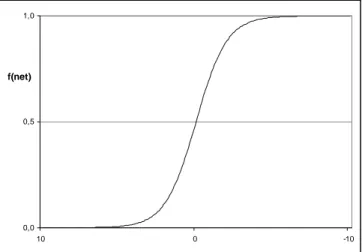
that can be used. The sigmoid function

net e net f ₋ + = 1 1 ) (

is the most common activation function for use in ANN; especially for backpropagation algorithms hence it is nonlinear, continuous and differentiable (Figure 3). It is nonlinear so that the shapes formed in feature space contain curves as

well as straight lines, which helps to solve linearly inseparable problems2. The sigmoid

function has a graded output; it is a smooth continues function where the function output is within the range of 0 to 1.

0,0 0,5 1,0

10 0 -10

f(net)

Figure 3. The sigmoid function. The x-axis show the weighted sum, the y axis the value returned by the function.

(11)

2.1.2 Supervised Learning Using the Backpropagation Algorithm

There are some different ways of training an ANN; in this dissertation only supervised learning will be considered. In supervised learning, the weights of the network are modified in order to decrease the deviance between the desired output and the output provided by the network for a given input pattern. When the network

consists of only one layer of connections, this learning method is known as the delta

rule. The backpropagation algorithm is often referred to as “generalized delta rule”

where delta is the error between desired and actual output that propagates back through the network (Rumelhart, Hinton and Williams 1986).

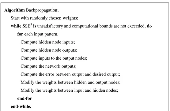
The feedforward process involves presenting an input pattern to input layer neurons that pass the values into the first layer. Each of the hidden layer nodes computes a weighted sum of its input, passes the sum through its activation function and presents the result to the output layer. In the output layer the input pattern are compared to the desired output; then the error are propagated back trough the net and the weights between the nodes are updated in order to minimize the total error. Networks are trained in three phases: Feed the data through the network, compute the error (backpropagation) and update weights (Mehotra et al. 1997). Figure 4 demonstrates the steps of the backpropagation algorithm.

Figure 4. Backpropagation algorithm (adapted from Mehotra el al., 1997, p.76).

For an extensive description of the backpropagation algorithm see Rumelhart, Hinton and Williams (1986).

3

Summed Squared Error: The squared error between actual output and target (desired) output for all output units. SSE=

∑

(o−t)2where o is the actual output and t is the target output. There are other error functions that can be used e.g. Mean squared error, Euclidian distance, Hamming Distance. There are also error functions that are based on evaluation of different classifiers. Further information about error functions can be found in Mehotra et al. (1997).

Algorithm Backpropagation;

Start with randomly chosen weights;

while SSE3 is unsatisfactory and computational bounds are not exceeded, do

for each input pattern,

Compute hidden node inputs; Compute hidden node outputs; Compute inputs to the output nodes; Compute the network outputs;

Compute the error between output and desired output; Modify the weights between hidden and output nodes; Modify the weights between input and hidden nodes;

end-for end-while.

(12)

2.1.3 Recurrent Networks

One drawback with the conventional feed-forward structure is that it does not allow sequential representations to be expressed very naturally (Adamson & Damper 1999). In some cases, such as time series predictions it is important to detect time dependent features in the sequence of input patterns. One way of doing so is to extend the input layer with additional nodes in order to present several patterns at the same time to the network. One can visualize the input layer in order to present several patterns at the same time. This strategy was used with success when Sejnovski & Rosenberg (1986) implemented NETtalk. NETtalk is a network that takes strings of characters forming English text and converts them into strings of phonemes that can serve as input to a speech synthesizer. The problem with these kinds of solutions is that they require that the user knows the appropriate size of the window; that is what the minimum number of symbols sufficient to extract time dependent features. Furthermore the window size is constant and the network has many synaptic weights that must be estimated.

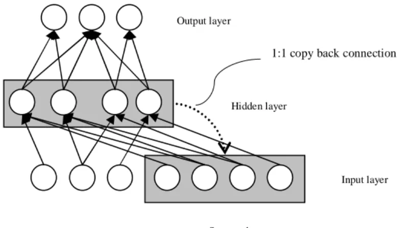
Elman (1990) pointed out that time are clearly important in cognition and are inextricably bound to many tasks with temporal sequences. Elman’s solution to detect time dependent features is to introduce recurrent connections from the hidden layer back to the input layer (Figure 5).

Figure 5. Elman’s (1990) recurrent neural network. The hidden layer activation is copied back to the states nodes in the input layer.

At each iteration a copy of the last hidden layer activation is transferred into a same-sized set of state nodes in the input layer. This is then used alongside the next input pattern to provide a memory of past events. Elman (1990) demonstrated a set of simulations which range from relatively simple problems (like a temporal version of the XOR problem) to discovering syntactic/semantic features for words. With a ‘simple sentence’ problem when the (trained) hidden units were examined and arranged into a tree hierarchy based on their activation, the network was observed to have organized the dictionary into syntactic categories. This indicates that knowledge captured in ANN’s is examinable, and contains meaningful/useful information (Elman 1990).

Hidden layer

Input layer

State nodes Output layer

(13)

2.2 Recursive Auto-Associative Memory (RAAM)

Pollack (1990) introduced the RAAM architecture which can represent variable sized symbolic sequences or trees in a numeric fixed-width form, suitable for use with association, categorization, pattern recognition and other neural-style processing mechanisms. The main advantage with this architecture is that even if the sequences presented to the network can vary in size, the network itself does not grow, but is still able to hold the different representation.

The idea with RAAM is to combine representations of previous input with current input. The data structure is fed sequentially to the network and the distributed representation contains representations of earlier inputs which makes the resulting

representation recursive.

The general RAAM architecture is a three-layer feed-forward network of processing units; the different layers are: input layer, output layer and hidden layer.

The set of connections between the input and hidden layer serve as encoding

mechanism and the connections between hidden layer and output layer serve as

decoding mechanism (Figure 6, Figure 7).

Figure 6. On the left the encoder network, to the right the decoder network. The encoder is a single layer network with 2n inputs and n outputs. The decoder is a single layer network with n inputs and 2n outputs.

Hidden Layer Hidden Layer Whole Left Right 2n input units n output units Whole Left Right 2n output units n input units

(14)

Figure 7. The RAAM network is composed of both encoder and decoder.

The input layer and output layer consists of equal number of units to allow

auto-association, of the pattern presented to the network. That is, the network is trained to

reproduce a set of input patterns; i.e. the input patterns are also used as desired (or target) patterns. In learning to do so, the network develops a compressed code on the hidden units for each of the input patterns.

In order to find codes for trees, however, this auto-associative architecture must be used recursively. For example, the network could be trained to reproduce (AB), (CD), and ((AB)(CD)) as follows:

Input pattern Hidden pattern Output pattern

(A B) → R1(t) → (A’(t) B’(t))

(C D) → R2(t) → (C’(t) D’(t))

(R1(t) R2(t)) → R3(t) → R1(t)’ R2(t)’)

Table 1. RAAM trained to reproduce (AB), (CD) and ((AB)(CD)) where t represent time, or epoch, of training (adapted from Pollack ,1990 , p.8).

The back-propagating learning algorithm is used to perform auto-association. Furthermore, the hidden layer must consist of fewer nodes than the input and output layer combined, in order to force the network to accomplish the auto-associative mapping by creating compressed hidden representations. Figure 8 illustrates an example of training a RAAM network to reproduce the tree structures: (AB), (CD), and ((AB)(CD)). n hidden units Whole Left Right 2n input units 2n output units Left Right Hidden Layer

(15)

Figure 8. Training a RAAM network to reproduce a tree structure. First the network is trained on one branch of the tree [AB]. Then the network is trained on the other branch of the tree [CD]. At last the network is trained to reproduce the whole tree [AB CD]. The drawings at the bottom of the figure illustrate the encoder and decoder part of the network.

[AB] A B C D A 1000 B 0100 C 0010 D 0001 [CD] C D C D 0 0 0 1 1 0 0 0 0 0 0 1 1 0 0 0 [ABCD] [AB] [CD] [AB] [CD] A B A B 0 1 0 0 0 0 1 0 0 1 0 0 0 0 1 0 A B Encoder [AB] [AB] A B Decoder

(16)

2.2.1 Sequential RAAM

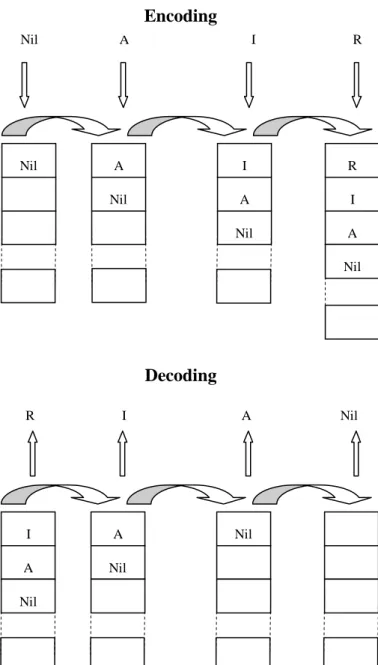
Pollack (1990) points out that sequences can be represented as left-branching trees, e.g. the sequence AIR can be represented as ((nil A)I)R). He also developed the sequential RAAM which is a slightly restricted version of the general architecture. An analogy to the sequential RAAM would be a stack. To explain what a stack is one can

use the Cafeteria plate holder as an analogy. In a cafeteria plate holder you can only

take the top plate (pop); when you take the top plate the others raise to the top and

when you add more plates you put them on the top (push). In short a stack is a

Last-In-First-Out access mechanism (Figure 9).

Figure 9. Last – In - First – Out mechanism. Encoding a symbol into the hidden layer of RAAM is analogous to adding a plate to the cafeteria plate holder, the symbol is pushed onto the hidden

Nil A Nil Nil A I A Nil I R I A Nil R Nil R I A Nil A I A Nil Nil Decoding Encoding

(17)

Figure 10. On the left, the encoder combines the m-dimensional representation for a sequence (Stack) with a new element (Top), returning a m-dimensional vector. To the right, the decoder decodes it back to its components.

Learning to represent a stack involves, for example to show training examples one

at a time to the RAAM. The encoding step is like the stack push operation and the

decoding step is like the stack pop operation (Pollack 1990; Blank et al 1991). When a

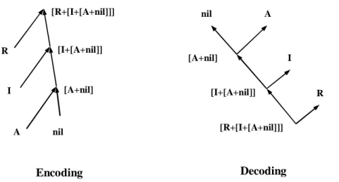
sequence of elements is compressed, the next element to be pushed, plus the stack is given to the RAAM as input (Figure 10). It then creates an updated version of the stack, containing the new element on the hidden layer. When a sequence is decoded, the representation of the stack is placed on the hidden layer. The topmost element and the remainder of the stack are produced as output (Figure 10). Figure 11 illustrates the encoding and decoding of a sequence, it also demonstrates that RAAM is acting analogous to a stack.

Figure 11. Encoding and decoding in RAAM: The left picture illustrate the encoding of the sequence AIR, and the right picture illustrates the decoding of the same sequence.

[A+nil] [A+nil] [I+[A+nil]] [R+[I+[A+nil]]] nil A R I A nil Decoding Encoding [I+[A+nil]] I [R+[I+[A+nil]]] R Hidden Layer Stack Top Stack n+m units m units Hidden Layer Stack Top Stack m units m+n units

(18)

Figure 12 illustrates the operation of the encoder, and Figure 13 illustrates the operation of the decoder network for a sequential RAAM, which, when viewed as a

single network has n+m input and output units, and m hidden units. When decoding, a

terminal test is normally performed on the decomposed representations to see if any of them is an atomic representation and should not therefore be decompressed any

further. An m-vector of all 0.5’s is chosen by Pollack (1990) to represent nil, the

empty sequence, which, according to Pollack, is very unlikely ever to be generated as an intermediate state. Other successful ways to represent the terminal element has also been presented (Chalmers, 1990; Niklasson & Sharkey, 1992).

When the network is trained with the patters:

Input pattern Hidden pattern Output pattern

(nil R) → D1(t) → (nil’(t) R’(t))

(D1(t) I → D2(t) → (D’1(t) I’(t))

(D2(t) A → D3(t) → (D2(t)’ A’(t))

Table 2. RAAM trained to reproduce the sequence AIR where t represent time, or epoch, of training.

It is expected that after backpropagation converges, D3 will be the representation for

the sequence (AIR). Representations will also be developed for all prefixes to the sequence, in this case (A) and (AI).

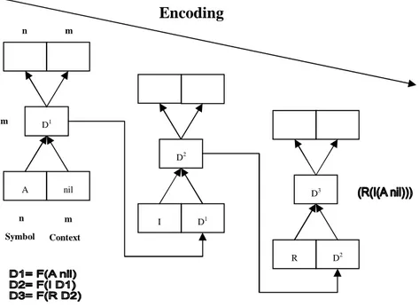
Figure 12. Encoding distributed representations in RAAM. The network is viewed in three different time-steps encoding sequence AIR.

D2 I D1 D3 R D2 D1 A nil n Symbol m Context n m m Encoding

(19)

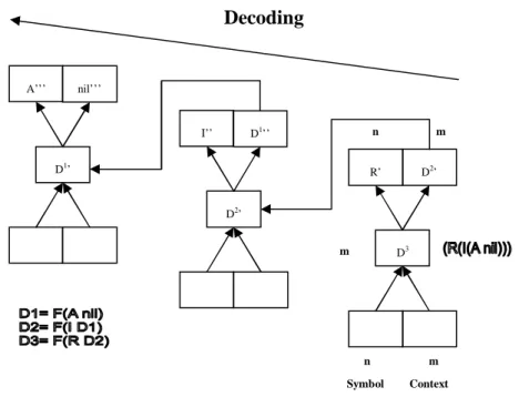
Figure 13. Decoding distributed representations in RAAM. The network is viewed in three different time-steps decoding the sequence AIR. Decoded representations are denoted ’, ’’ and ’’’. Representations are seldom decoded to its exact original state since there are inaccuracies in the decoding process.

There is no fixed limit on the number of patterns that can be encoded by the network. The error rate of the network when encoding sequences, is influenced by the length and the numbers of sequences, the complexity of the domain of which the sequences are derived and the number of hidden units employed (Pollack 1990).

As a conclusion, Pollack’s RAAM consists of two separate mechanisms, an encoder and a decoder, which evolve simultaneously and work together to develop a shared representation. The encoder produces a fixed length representation for a sequence which the decoder can decode and reconstruct into a facsimile reproduction of the original. The hidden layer represents the sequence, which demonstrates how a fixed architecture can indeed accommodate variable-sized data structures (Pollack 1990; Blank et al 1991).

2.2.2 Local versus Distributed Representations in RAAM

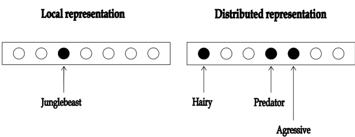
A local representation in a RAAM network is when the network is designed so that individual inputnodes in the network denote particular concepts. For example one node stands for ‘chimp’, another for ‘cheetah’ another for ‘rhino’ and so on. A distributed input-representation is when one unit take part in representing more than

one concept e.g. predator yes/no, hairy yes/no. When a concept is distributed it means

that it appears as a distributed pattern of activity. The left field of the input units in a

sequential RAAM act as local representations when the terminal vectors are

orthogonal: a single element in the terminal vector has the value 1 and so a single unit

will be switched on. The compressed representation that develop on the hidden units are usually distributed in that a single letter from a word sequence, for example, is represented by more than one hidden unit. According to Callan (1999) a distributed

R’ D2_’ D3 I’’ D1_’’ D2_’ A’’’ nil’’’ D1’ n Symbol m Context n m m Decoding

(20)

architecture is more economic than a local for representing concepts. For example, a

network with n binary units can only represent n concepts locally, whereas a

distributed architecture can represent 2n binary patterns.

RAAM has in different experiments shown a powerful ability to act upon holistic

representations. Using different variations of RAAM in conjunction with other simple feed-forward networks has exhibited detectors, decoders and transformers which act

holistically on the distributed, sub-symbolic symbols created in RAAM (Blank et al

1991; Chalmers 1990; Chrisman 1991; Bodén & Niklasson 2000). In a holistic computation the constituents of an object are acted upon simultaneously, rather than on a one-by-one basis as is typical in traditional symbolic systems (Hammerton. 1999). In this way, a subsymbolic operation can, in one step, perform a complex function without decomposing the representation of a symbol structure into its constituent parts (Blank et al 1991).

Figure 14. Local and distributed representations of the concept Junglebeast. In the local representation one single node denote the concept Junglebeast. In the distributed representation units takes part in representing more than one concept, and a concept is represented by more than one unit.

(21)

2.3 Bi Coded RAAM (B-RAAM)

Pollack (1990), Blank et al (1991), Chalmers (1990), Chrisman (1991), Bodén & Niklasson (2000) and others have uncovered that the ability for RAAM to operate on holistic representations is very powerful. RAAM is useful for its ability to generalize, as a result of learning, so that it can encode and decode novel data structures. Despite the power and flexibility of RAAM, Adamson & Damper (1999) points out some of its shortcomings:

Scalability: RAAM does not scale up to large structures.

Moving Target Problem: It takes RAAM many epochs to learn the

representations. One reason is that the hidden layer activations are part of both the input and target pattern. The input and output patterns constantly change as a result of hidden-layer feedback.

Long Term Dependency Problem: RAAM, as any other recurrent network,

exhibits a bias towards the most recently seen symbols in a sequence. The RAAM network makes less error for later symbols than for earlier symbols in a sequence.

Noise Sensitivity: The recursive process required to decode holistic

representations of sequences suffers a cumulative error effect. Since decoding is a recursive procedure it accumulates and amplifies errors of the representation and is therefore very noise-sensitive.

Time Consuming: Training RAAM networks is time consuming, partly because

of the moving target problem and the cumulative error effect.

The solution to these problems is according to Adamson and Damper (1999) the Bi coded RAAM architecture (B-RAAM). B-RAAM (Figure 15) is a modification of the original RAAM architecture. It introduces a new output mechanism and a delay line which according to Adamson & and Damper (1999):

Speeds up the learning process.

Computes smaller-sized representations. Improves in remembering earlier inputs.

(22)

Figure 15. The B-RAAM architecture. In the output sequence all the symbols in the encoded sequence are decoded at once. We can also see the delay line, in which the hidden layer from several previous steps in the sequence is re-fed into the network (remake from Hansson & Niklasson 2001).

Bi coded RAAM differs from Pollack’s RAAM in its use of bi-coding. Adamson & Damper’s (1999, p.49) explain what bi-coding means.

“Because although the same information is present within both the input and output layers during each cycle, it is represented in two different ways. First the output layer is dynamic and comprises a concatenation of external input patterns- in this case hand-coded, although any sensible representation can be used. Second the input layer representation comprises an encoded sequence of fed-back data (taken from the hidden layer and the current external pattern (next symbol).”

In contrast to the recursive decoding of RAAM, the sequence is decoded at once. During learning of a sequence the first symbol is presented to the network as output and target pattern. In the second step the next symbol is presented as well as the hidden layer activations the same as in RAAM, but now the target is the current symbol at the node where the previous symbol was and the previous symbol is shifted to the left. After the whole sequence is presented it can be “read” at the output layer. The number of output nodes increases as longer sequences arrive. This way of decoding reduces the moving target problem because only the input pattern changes through training. The output is also allowed to grow dynamically with the sequence (Figure 16), whereas in RAAM, the size of the output nodes is fixed.

New symbol

Delay line

Output sequence

Copy 1:1

(23)

Figure 16. B-RAAM associates a time-delayed encoder input (partly drawn from the hidden layer) to its decoded constituent parts during learning. This contrasts with RAAM, which is a strict recurrent AA (remake from Adamson & Damper 1999, p.48).

As already mentioned Adamson & Damper also introduced a delay line within the input layer, into which previous hidden layer activations was placed. The network

keeps the hidden layer activations of one sequence for x steps and feeds them back to

the input. After one step they are shifted, so that the oldest one is lost and a new one takes that place. According to Adamson & Damper (1999), the delay line allows the state information to persist for longer; earlier presented data in a sequence has an increasing effect on learning, because earlier presented data takes more part in the weight-adjustments, which reduces the bias towards later inputs.

B-RAAM takes into account the size of the sequences being processed, increasing the output layer as longer sequences arrive. Training is also directed precisely where it is appropriate. For example, a three letter sequence will only update the weights connected to the first three nodes of the output layer, irrespective how large it has grown to accommodate longer sequences. This technique, even though B-RAAM uses a larger architecture in some cases, using a dynamic output layer and a localized thresholding during training means that a significant reduction in weight calculations is achieved compared to RAAM.

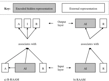
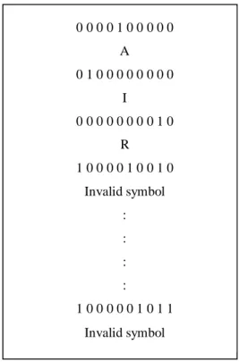
Encoding is achieved for B-RAAM by presenting sequence/tree elements one at a time until the complete sequence/tree has been seen. The holistic hidden-layer representation is then extracted. Decoding is even more straightforward, in that the holistic code need only be placed in the hidden layer and fed from this point once. The result should be a sequence of symbols at the output layer representing the constituent parts of the encoded sequence. In order to identify meaningful output i.e. output that represent a valid symbol, a subnetwork can be trained on sequence-length association. If an output pattern is decoded and it does not represent a valid symbol, this output pattern indicates the end of the sequence; accordingly, the symbol preceding this invalid output pattern is the last in the sequence. For example, all valid symbols are orthogonal represented with one node as 1 plus the others as 0, and an output pattern is decoded that contains more or less than one node as 1, this output will not be a valid

Encoded hidden representation External representation

AI A R associates with A I R Key: Input layer AI R associates with AI R Output layer a) B-RAAM b) RAAM

(24)

symbol and therefore indicate the end of the sequence (Figure 17 and Figure 18). The subnetwork is only mentioned by Adamson & Damper and none of the details are described. There are no information about the architecture of the network, neither is it described how the network is trained. This is a sharp criticism directed to authors of scientific publications in general and to Adamson & Damper in particular. Published science material should contain sufficiently many details, allowing others to repeat the experiments.

Figure 17. An example of an output for the sequence (AIR) in a B-RAAM network with more than three outputnodes.

A R Not used to

represent sequence

Hidden nodes I

Updated weights Weights not updated

Output nodes 0 0 0 0 1 0 0 0 0 0 A 0 1 0 0 0 0 0 0 0 0 I 0 0 0 0 0 0 0 0 1 0 R 1 0 0 0 0 1 0 0 1 0 Invalid symbol : : : : 1 0 0 0 0 0 1 0 1 1 Invalid symbol

(25)

A limitation however with the B-RAAM architecture is that the training-set has to involve the longest sequence. If a sequence is presented to the network, which consists of more symbols than any of the sequences the network has been trained on, the network cannot decompose that sequence. The reason for this is that the number of output nodes increases during training, as longer sequences arrives.

Figure 19 illustrates B-RAAM encoding the sequence (A(I(R nil))). The delay line improves the network’s ability in remembering earlier inputs.

Figure 19. Encoding distributed representations in B-RAAM. The network is viewed in two different time-steps encoding sequence AIR. The dotted line illustrates the time delayed encoder input which encodes the hidden layer from previous steps in the sequence. In this example the delay line is set to one.

Figure 20 illustrates B-RAAM decoding the sequence (A(I(R nil))). As can be seen, the whole sequence is decoded in one step. One of the major disparities between RAAM and B-RAAM is that in RAAM the elements are chained to each other in the hidden representation, this is not the case in B-RAAM. When decoding a sequence back to its constituents in RAAM the most recent encoded element needs to be decoded first in order to reach the element encoded before that, and so on until all elements are decoded. In B-RAAM the elements are not chained together in the hidden layer, and therefore all elements can be decoded in arbitrary order.

D1= F(A I) D2= F(R D1) Encoding (A(I(R))) D2 R D1 A n Symbol m Context D1 I A m -

(26)

Figure 20. Decoding distributed representations in B-RAAM. The network is viewed in decoding the sequence AIR. B-RAAM decodes the whole sequence in one single step.

As a conclusion it can be said that the encoder networks are identical in both RAAM and B-RAAM. The decoder network in the two architectures is on the other hand much dissimilar; it is two totally different techniques that are used. Instead of decoding the sequences in a recursive manner as in RAAM, B-RAAM decodes the sequences in one step. Furthermore, in B-RAAM the encoded sequences are not reproduced on the output layer in an auto associative manner like in RAAM. In B-RAAM the hidden encoded representation associates to all the encoded symbols unlike RAAM were the hidden representation associates to one extracted symbol and the rest of the sequence compressed, precisely as it is encoded.

n Symbol m Context m Decoding D3 A I R (A(I(R))) -

(27)

2.4 Related Work

This section briefly overviews the current research in the area. The intention of this chapter is to describe the various different types of RAAM architectures and experiments performed with these. The different architectures are described and discussed separately, each in one subsection. Note that there also exists other extensions to RAAM that is not mentioned in this work.

2.4.1 Two Layer Digital RAAM

Blair (1995) introduced the Two Layer Digital RAAM. Blair’s idea was to introduce two extra layers to the RAAM to increase robustness and storage capacity. One extra layer where located between the input layer and the encoded layer, and the other where located between the encoded layer and the output layer. Blair (1995) also tried to deal with the problem of accumulated errors in during decoding.

One problem with RAAM according to Blair (1995) is that, since the representations are allowed to take non-integer values greater accuracy is required as the depth of the trees increases, in order to round-off errors. Therefore Blair (1995) modified the network so that each output must take a discrete value (+1 or -1), thus allowing deeper structures to be stored in a noise tolerant fashion. By contiguously setting all output units to binary digits Blair removed the error at each encoding and decoding step and hence it never got so big that it affected the result. The training was the same that in an ordinary RAAM apart from that the backpropagation algorithm was substituted with a similar quickpropagation algorithm (Fahlman 1989).

2.4.2 Extended RAAM (E-RAAM)

E-RAAM was originally suggested by Nicklasson and Sharkey (1992) and is an extension of the RAAM architecture. When decompressing, a terminal test is normally performed on the decompressed representation to see if any of them is a terminal and therefore not be further decompressed. The terminals contain the representation of the items in sequence. There are different solutions suggested for this terminal test (see Chalmers (1990); Pollack (1990)). The solution suggested by Niclasson and Sharkey (1992) in the E-RAAM architecture was to add an extra bit of information to each part of the sequence. If the representation is a terminal the extra bit is set to1 otherwise it is set to 0.

(28)

Figure 21. ERAAM structure. The extra bit in the input and an output layer is used to classify if the representation is a terminal or a composite structure (adapted from Hansson & Niklasson 2001, p 2).

2.4.3 Dual-Ported RAAM

The dual ported RAAM is an architecture developed by Chrisman (1991). What

Chrisman was doing was to merge representation and processing by using confluent

inference, so that the processing of the sequence took place at the same time as the

sequence where being represented. So, if the input for an inference is x and the desired output is f(x) then the confluent inference tries to encode both x and f(x) simultaneously in the representation of x. According to Chrisman confluent inference achieves a tight coupling between the distributed representations of a problem and the solution for a given inference task while the net is still learning its representations. The benefit of this, according to Chrisman is that the representation for a sequence support the processing of it.

2.4.4 Recursive Hetero-Associative RAAM (RHAM)

Forcada & Neco (1997) agreed with Chrisman’s (1991) idea that the processing task should be supported by the representation of a sequence. However, they did not agree that the representations should be the same for its original sequence and the resulting sequence. RHAM is capable of learning simple translation tasks, by building state-space representation of each input string and then unfolding it to obtain the corresponding output string. This way the encoding representation could be directly decoded into the resulting sequence.

Step 2 Step 1 1 d1 a’ b’ 1 1 a b 1 1 d2 c’ d’ 0 1 c d1 0

(29)

3. Problem Description

In this chapter the problem of interest will be described. First an overview of the

problem will be given, and then in the problem delimitation section the focus of the

problem will be described.

3.1 Problem Domain

Since Pollack (1990) introduced the RAAM architecture there have been many extensions to it, in order to achieve better performing RAAM-based architectures (Chrisman 1991, Niklasson & Sharkey 1992, and Blair 1995).

This dissertation investigates the B-RAAM architecture developed by Adamson & Damper (1999). The architecture was presented in 1999; some time has passed since then, and the architecture has not so far made any great impact on the research community. There can be different reasons why the B-RAAM has not been brought into attention: Lack of use for it, poor performance, lack of biological plausibility or the fact that no one has discovered its benefits, may be some possible reasons.

Adamson & Damper (1999) describe B-RAAM as a promising extension of the RAAM architecture and they state some advantages over RAAM, these advantages they also verify experimentally. In their experiments much emphasis is put on the severity of bias towards recent decoded symbols and on the effect of noise in input. They use representations that are produced with the motive of verify that B-RAAM is less sensitive to noise, and that B-RAAM improves in remember earlier inputs. Therefore, in this dissertation an experiment with a generalization task is performed to compare the two architectures. This will hopefully broaden the view of B-RAAM and give light to the claims of Adamson & Damper (1999). Moreover, no one has up to now explored the internal representation of B-RAAM. With this in mind there is reason to conduct further studies on B-RAAM.

Blank et al. (1991) have completed an exhaustive case study on RAAM by conducting a series of experiments. By replicating one of the experiments conducted by Blank et al. (1991), a comparison can be made between B-RAAM and RAAM.

The aim of this dissertation is to carry out an exploratory study on B-RAAM; to see how well the network generalizes, look for advantages and disadvantages, measure the performance, and to briefly explore the internal representation. In addition to this, theoretical issues on RAAM and B-RAAM will be discussed.

(30)

3.2 Problem Delimitation

This dissertation focus on some of the factors that Adamson & Damper (1999) describes as making the most significant advantages of B-RAAM over RAAM. To investigate those factors, one experiment, showing RAAMs ability to generalize, will be replicated on RAAM and B-RAAM and the architectures will be compared.

Adamson & Damper (1999) states that in their experiments did B-RAAM improve over RAAM in the following ways.

B-RAAM:

Speeds up the learning process. This will be investigated by comparing number

of epochs needed in training for the network to learn the training set.

Computes smaller-sized representations. This will be investigated by comparing

number of internal nodes needed to solve a defined task.

Improves in remembering earlier inputs. That claim will not be investigated

here. Adamson & Damper (1999) investigated it by comparing the two architectures to see if B-RAAM makes fewer errors on early input of a sequence than RAAM.

Solves the problem of cumulative decoding errors. That claim will not be

investigated here. Adamson & Damper (1999) investigated by introduce noise into the input and present it to the B-RAAM architecture to see how it affects the performance.

In this dissertation three properties of B-RAAM will be investigated:

The effect the number of internal nodes has on learning and generalization. Number of training epochs needed to learn the training set.

The networks ability to generalize.

The number of internal nodes is pertinent as a measurement of representation size

hence it shows how much the network can compress the encoded sequences and still be able to decode them back to its constituents. Using less number of nodes result in fewer weight updates, which speeds up the training process. Smaller network architectures result in more effective compression of data and speeds up learning.

Number of epochs needed in training to learn the training set is one possible

measurement of training speed; few epochs needed in training speeds up training phase. One of the main concerns of the RAAM architecture is the fact that training is very time consuming. It is obvious that a network with a few nodes, trained with few epochs is more effective than a network with many nodes, trained with many epochs.

Ability to generalize: Generalization is a term used to refer to how well a network

performs on data from the domain which it has not been trained on. For instance, a supervised trained network with good generalization would be expected to classify

(31)

All the three properties mentioned above may be dependent on each other. Poor generalization can for example be due to having either too few internal nodes or too many. Too many internal nodes will probably lead to that the network memorizes the training set, which leads to poor generalization capabilities. Too few internal nodes, on the other hand, will result in that the weight space cannot include all the different representations. Overtraining with too many hidden units means that the network fits the training data too well and there is not enough allowance for new samples that vary from the training samples (Callen 1990).

In summary, the main objective in this dissertation is to investigate the effect the number of internal nodes has on learning and generalization, the number of training epochs needed to learn the training set and the ability to generalize for B-RAAM and for RAAM. The performance measure will hopefully illuminate some of the advantages and disadvantages of B-RAAM.

To reproduce the entire experiment from Blank et al. (1991) completely the secondary objective of this dissertation is to examine the internal representation of B-RAAM and to compare it to the internal representation of B-RAAM. The intention is not to make a detailed study of the internal representation, but to get a notion of how the internal representations differ between the two networks. Comparison using the hierarchical cluster analysis will be made to get an understanding of how the internal representations look like in B-RAAM and in what way it is different from the internal representation of RAAM. Hierarchical cluster analysis is used as a statistical method for finding relatively homogeneous clusters of cases based on measured characteristics. There are hierarchical cluster analyses in Blank et al. (1991) produced from the RAAM architecture in order to examine RAAM’s ability to generalize more directly. The aim is to reproduce those on RAAM and B-RAAM to compare and analyse them to see if B-RAAM generalizes in a similar manner as RAAM.

(32)

4. Experiments

In this section the experiments conducted in this dissertation will be presented. Section 4.1 describes the simple sentences encoding experiment. Section 4.2 describes the modifications that have been made on the B-RAAM architecture. Finally Section 4.3 describes Hierarchical cluster analysis and reveals some of its benefits and shortcomings.

4.1 Encoded Simple Sentences

Blank et al. (1991) explored RAAM’s potential more fully, and they devised a set of experiments where simple sentences were encoded. A corpus of two and three words sentences was created using a slimmed-down version of a small grammar

created by Elman (1990) which he called Tarzan grammar (explained below), and

then decoded by a sequential RAAM.

Blank et al. (1991) created two and three word sentences from a set of 26 words (15 nouns and 11 verbs); one stop word was also created to indicate the end of a sequence. The words were described by lexical categories (Table 3). Blank et al. (1991) also created templates that specified in what way the lexical categories could be combined (Table 4). The grammar restricted the number of valid sentences to 341 from a total of 18,252. To represent the different words as input to the RAAM, Blank et al. (1991)

assigned to each word an individual code that consisted of 27 bits. They used a localist

representation (see Section 2.2.2); for each word, one bit was on, the others off. The corpus consisted of 100 unique sentences to be used for training and another 100 to be used for generalization tests.

This experiment will be replicated on RAAM and B-RAAM to see the difference in performance between the two architectures. Furthermore, the development of generalizations within the two architectures will be examined and compared. A cluster analysis based on Euclidian distance will be performed on the encoded representations of the 100 trained sentences.

4.1.1 Creation of Sentences

Two and three words English-like sentences were generated from a set of 26 words (15 nouns and 11 verbs). An additional word, stop was used to indicate the end of a sentence. The words where divided into different lexical categories as shown in Table 3. Note that one word can be a member of more than one lexical category, e.g. the

word Tarzan is a member in five different categories (ANIMATE,

NOUN-MOBILE, NOUN-SWINGER, NOUN, NOUN-REAL) and smell is a member in two

different categories (VERB-PERCEIVE, VERB-INTRANS). The sentence templates

given in Table 4 specify in what way the lexical categories could be combined to form sentences. As can be seen in Table 4 sentences where either in the form (NOUN

(33)

Category Members

NOUN-ANIMATE tarzan, jane, boy, cheetah, chimp, rhino

NOUN-AGGRESSIVE cheetah, rhino, bigfoot, junglebeast,

NOUN-EDIBLE coconut, banana, berries, meat

NOUN-SQUISH banana, berries

NOUN-MOBILE NOUN-ANIMATE + (bigfoot, junglebeast, jeep)

NOUN-SWINGER tarzan, chimp

NOUN-HUNTER jane

NOUN NOUN-ANIMATE + (bigfoot, junglebeast) +

NOUN-EDIBLE + (jeep, tree, rock)

NOUN-REAL NOUN – (bigfoot, junglebeast)

VERB-FLEE flee

VERB-HUNT hunt

VERB-AGRESS kill, chase

VERB-SQUISH squish

VERB-MOVE move

VERB-EAT eat

VERB-PERCEIVE see, smell

VERB-INTRANS see, smell

VERB-EXIST exist

VERB-SWING swing

Table 3. Categories of lexical items used in simple sentence generator (adapted from Blank et al. 1991).

Table 4. Templates used in the sentence generator (adapted from Blank et al. 1991).

Template Word1 Word 2 Word 3

1 NOUN-ANIMATE VERB-FLEE NOUN-AGGRESSIVE

2 NOUN-AGGRESSIVE VERB-AGRESS NOUN-ANIMATE

3 NOUN-ANIMATE VERB-SQUISH NOUN-SQUISH

4 NOUN-ANIMATE VERB-EAT NOUN-EDIBLE

5 NOUN-ANIMATE VERB-PERCEIVE NOUN

6 NOUN-MOBILE VERB-MOVE 7 NOUN-ANIMATE VERB-INTRANS 8 NOUN-REAL VERB-EXIST 9 NOUN-SWINGER VERB-SWING 10 NOUN-HUNTER VERB-HUNT 11 NOUN-AGGRESSIVE VERB-HUNT

(34)

Template Example sentences 1 rhino flee junglebeast 2 cheetah kill jane 3 tarzan squish banana 4 boy eat coconut 5 bigfoot see jeep

6 chimp move 7 tarzan smell 8 tree exists 9 chimp swing 10 jane hunt 11 junglebeast hunt

(35)

4.1.2 Experimental Setup

All the networks were trained with 100 sentences created in the sentence generator. A test set where also created containing 100 sentences (Blank et al. 1991). The networks where then trained on the training sentences for 21000 epochs (Blank et al. 1991). After every 50th epoch of training the networks ability to generalize was tested, both training sentences and test sentences were encoded and decoded and then it was measured how many of the sentences the network was able to decode correctly. The tests were conducted by encoding one sequence at a time and than decode it and compare it to the desired output sequence. During testing the weights where freezed and no training was performed.

4.1.3 Choice of Parameters

There are some practical issues that have to be considered when training RAAM networks. The performance of the network is much dependent on what choices are made. The only parameters that are changed during the experiments is the network topology, all the other parameter are fixed. To find optimal settings for all the different network topologies the other factors that influencing the performance of the network probably also has to be changed. For example, the settings for the learning algorithm may be suitable for one of the larger topologies, but not for one of the smaller topologies. Training and test set will probably also affect the outcome of the experiments, some training and test sets are perhaps suitable for some topologies but not for others. In these experiments however, the parameters are the same for all experiments with all the different network topologies.

Weight Initialization

Weight initialization is one of the issues that have to be considered. Weights are usually initialized to small random values, e.g. within the interval [-1.1] or [-0.1,0.1] (Mehotra el al.1997). Larger weights may slow down initial training because of the low derivates of the sigmoid function. In these experiments initial weights between [-0.5,0.5] were used.

Learning Method

According to Mehotra et al. (1997) there are two approaches to learning. “Per

pattern learning”: when weights are changed after every sample presentation and “per epoch learning”: weights are updated only after all samples are presented to the

network. In these experiments networks are trained with per pattern learning.

Learning Rate and Momentum Parameter

The Learning rate is typically set to a low constant value, e.g. 0.01 or 0.1. When to

rapidly find the best possible solution (minimize the error) a large value are chosen as learning rate. Although using to large value on the learning rate will increase the risk that the optimal solution is missed. To fasten the learning process and to minimize the

risks of ending up in local minima a further value can be added the momentum

parameter. The momentum parameter can help to overcome the problem of local minima because the change in a weight includes a fraction of the previous weight

(36)

change. To see the effect of the momentum term, consider that the gradient decent search trajectory is analogous to a (momentumless) ball rolling down the error surface. The effect of the momentum parameter is to add momentum that keeps the ball moving in the same direction from one iteration to the next (Mitchell 1997). If the previous weight change resulted in a large downhill shift in the error, and the network is now in a local minimum, the previous weight change might help the network to continue on the downhill slope since there is enough momentum to overcome the small valley in the error landscape (Figure 22).

Figure 22. Attempting to avoid local minima by using momentum (adapted from Callan 1990 p. 139).

The weight change induced by pattern n+1 is dependent on the weight change induced by pattern n. The momentum parameter must have a value between 0 and 1; a value close to 0 implies that the past history does not have much effect on the weight change, while a value closer to 1 suggests that the error has little effect on the weight change. However, direction for weight change chosen in early stages of training can strongly bias future weight changes, possibly restricting the training algorithm to only explore one region of the weight space (Mehotra et al. 1997). However, for each of the architectures tested in these experiments, 15 networks are created with different initial weighs. It is very unlikely that the training algorithm would be restricted to explore the same region of the weight space for every network.

A well chosen value on the momentum parameter can significantly reduce the number of iterations for convergence (Mehotra et al. 1997). According to Mehotra et al. (1997) the optimal momentum value depends much on the application and is not

easy to determine a priori. Values for momentum parameter can, as well as the

learning rate, be obtained adaptively.

Since two network models are compared here it is considered best to give as similar basic condition as possible, therefore fixed values are chosen on both learning rate and momentum parameter. Neither the learning rate nor the momentum parameter was defined by Blank et al. (1991) which is a weakness, since makes it difficult to replicate the experiment. The networks in these experiments are trained for many epochs

Last weight change resulted in this drop in error. The network is now in a valley and potentially stuck. However, if a percentage of the last change is added via the momentum term, then the error might be forced to continue downhill.

(37)

Network Topology

Network topology is also an important factor to consider. Networks are not to be either too large or too small. A network with too many nodes may be capable of

memorizing the network instead of generalizing from data. A network with too few

nodes may not be powerful enough for a given learning task. Choices of network topologies for experiments in this dissertation are based on experiments in Blank et al. (1991). Since a network with a 27-30-27 topology solved the task in a sufficient way for Blank et al. (1991), topologies used in this dissertation are similar to 27-30-27 topology; only the number of internal nodes differs.

Network topologies of 15, 20, 25 and 29 internal nodes where trained and tested in this dissertation. The initial idea was to test network topologies of 15, 20, 25, 30 internal nodes. Due to restrictions in the implementation 29 internal nodes was chosen, 29 was the upper bond of possible internal nodes.

Training Set

How many samples are needed for good training? This is a difficult question whose answer depends on several factors, a rule of thumb, obtained from related statistical problems, is to have at least five to ten times as many training examples as the number of weights to be trained (Mehotra et al. 1997). Blank et al. (1991) has chosen 100 sequences in their training set, and therefore 100 sentences is also is used for experiments in this dissertation. According to the rule of thumb mentioned, a training set of 7830 to 15660 sentences would be needed in a 27-29-27 network as it contains 1566 weights.

Representation

The representation of data should be in a format suitable for the network. The representation should be unbiased and free from inconsistencies. Representations that require “extra” processing for the network should also be avoided. Blank et al. (1991) used an orthogonal representation for each word where only one node is set to 1 and the others are set to 0. The orthogonal representation is unbiased and free from

inconstancies since it has no microsemantics, which means that the symbols has no

internal relationship to each other.

The words and the sequences are randomly generated; therefore words and sentences used in these experiments most probably are not the same that Blank et al. (1991) used in their experiments. Certainly the training data is an important factor that has a big impact on the networks ability to generalize. Generating the sentences randomly may result in that data does not fully represent all possible states of the problem and that there are not sufficient data to allow test and validation sets to be extracted. The data selection for training must according to Callen (1999) be representative for the complete space a class might occupy. For example, if two classes are located very close to each other, it is important to include data from the boundary that separates the classes; otherwise samples from this region can be misclassified. Random selection is however unbiased and therefore it is a good chance that data representing most of the possible states of the problem are chosen.

(38)

The task performed in this experiment also involves a harder type of generalization as the network are tested on the ability to generalize to new sequences including words that has occurred in the training set, but not on that particular position in the sequence. The network can for example come across a sentence, in the test set, were the word

Tarzan occurs in the third position, even if the word Tarzan only occurs in the first

position in the training set.

To decrease the risk that the network is only trained one some states of the training data and tested on others, a number of different training and test set can be created. This was, however not done in these experiments, since it was not in done in Blank et al (1991).

(39)

4.2 Modifications of B-RAAM

The experiments in this dissertation are conducted with a B-RAAM architecture that differs some from the original one, presented by Adamson & Damper (1999). The architecture is modified in the following ways:

The delay line is not implemented

The network that decides the sequence lengths is not implemented; B-RAAM is trained to represent invalid symbols as null padding instead.

The delay line is not implemented since sequences encoded in the experiments are built up only with two or three symbols. The delay line was appraised not to be suitable, for these experiments, because the later elements would have to much influence in the representation. A 30 hidden node network would result in 900 additional weights for each introduced delay line; furthermore, it would result in that almost the entire sequence would be presented in a dedicated input at the final item. The purpose of the use of delay lines is that the network will improve in remembering earlier inputs; which is a property that is not in the focus of this dissertation.

The major difference between the architecture used in this dissertation and the one defined by Adamson & Damper is the training and the decoding procedure. In the original B-RAAM only weights of outputnodes that are involved in representing the encoded sequence are adjusted during training; the weights of outputnodes that are already created but not used to represent the current sequence are not updated (see section 2.3). This procedure prevents the network from learning null padding, i.e. train the outputnodes to represent a null element, which in these experiments contains only 0’s (Figure 23).

Training B-RAAM not to learn null patterns, like Adamson & Damper, results in that the network itself cannot identify the length of the sequence; some of the decoded symbols will be invalid and should therefore not be part of the output sequence. For example, a decoded sequence shorter than the longest sequence used in training will contain non-target symbols. The network itself cannot decide which symbols that are part of the sequence and which are not. Adamson & Damper solves this by adding an external subnetwork trained on sequence-length association (see section 2.3). The architecture used in this work is modified so that all weights are updated at every

training epoch to learn “null patterns” where no symbol should be present. The effect

of this change is that the network will learn null patterns, i.e. learn to decode non valid symbols as all 0’s (Figure 23). This means that two symbol long sequences in reality are three symbols long. Using this training method the “sequence length deciding subnetwork” is not needed since all patterns that contain only 0’s are not counted as a symbol.