B
ased Virtual Towers in CFD Simulations
Master of Science in Wind Power Project Management
By Roger Moubarak
Energy Technology at Gotland University
Supervisor: Dr. Bahri Uzunoglu
ABSTRACT
Gotland University
Faculty of Energy Technology
By Roger Moubarak
Energy Production Prediction using Global and Regional based Virtual Towers in CFD Simulations.
Master’s thesis, 2011
30 pages, 13 figures, 3 tables and 5 appendices
Examiners/Supervisors: Dr Stefan Ivanell, Dr Bahri Uzunoglu
Keywords: Global-Regional Global Model, Era Interim, StormGeo, WRF, ECMWF, Data Series, WindSim, Hindcast.
Wind farm assessment is a costly and time consuming process when it is planned by traditional methods such as a met mast. Therefore, new models have been established and used for the wind farm assessment to ease the process of wind farm planning. These models are Global-regional models which add to cost efficiency and time saving. There are several types of these models in the market that have different accuracy. This thesis discusses and uses in simulations Global – regional model data outputs from European Centre for Medium-Range Weather Forecasts (ECMWF), Weather Research Forecast WRF and ECMWF, which is currently producing ERA-Interim, global reanalysis of the data-rich period since 1989 .
The goal of the master's thesis is to see whether it is useful and efficient to use Global – regional weather model data such as the Era Interim Global Reanalysis Model data for wind assessment by comparing it with the real data series (met mast) located in Maglarp, in the south of Sweden.
The comparison shows that in that specific area (hindcast) at Maglarp, in the south of Sweden, very promising results for planning a wind farm for a 100m, 120m and 38m heights.
Acknowledgements:
I would like to thank my supervisor at the University of Gotland Dr. Bahri Uzunoglu for giving me help and support during the entire period of my thesis work.
Many grateful thanks to CEO of StormGeo in Sweden Johan Groth and Olav Erikstad, Key Account Manager, in Norway for giving me an opportunity for doing this thesis work for their company StormGeo.
Also a lot and grateful thanks to Daniel Fredriksson from the company StormGeo for his enormous assistance and for giving me his valuable time in answering my questions and providing me with all necessary data during the period of the thesis work.
I would also like to give thanks to Karin Bengtsson the vice rector of the Gotland University for helping me do the presentation of my thesis work.
A lot of thanks to Ola Eriksson for his help in the Wasp and Windpro software.
Many thanks to Hans Bergström for giving me data series of several locations in Sweden.
Many thanks to the University of Gotland and Stefan Ivanell in particular for listening to my presentation.
Last but not least, I greatly appreciate and thanks to my wonderful girlfriend Asta Glinskaite for helping me edit the English text of this thesis work.
Sincerely, Roger Moubarak Visby, June 2011
Table of Contents
1. Introduction……….5 2.Limitations / Delimitations………...6 3. Models………...6 3.1. CFD models………..6 3.1.1 WindSim……….63.2 Global- Regional weather model………...……...……….7
3.2.1 Differences / Advantages...……..………...7
3.2.2 ECMWF ………...………...7
3.2.2.1 How numerical weather prediction works ...………9
3.2.3 ERA………..………...10
3.2.4 The WRF model ……….………10
4. StormGeo………..………...11
4.1 The WRF Model (StormGeo)……...………...………...………...11
4.2 The ECMWF Model (StormGeo)…….………...………..13
5. Methodology ………..……….…14
5.1 Terrain module…...14
5.1.1 Map………..………...14
5.2 Wind fields module...15
5.3 Object………...……… 17
5.4 Wind resources………...……….. 17
5.6 StormGeo………..17
6. Results……….18
6.1 Differences in wind speed between two models with initial shooting height of ERA Interim based on WindSim of 38m………….………...19
6.2 Differences in wind speed between two models with initial shooting height of ERA Interim based on WindSim of 38m…..………...20
6.3 Differences in wind speed between two models with initial shooting height of ERA Interim based on WindSim of 38m.……….………...22
7. Uncertainty……….….23
8. Discussion………23
1. Introduction:
Wind farm planning is a time consuming process which requires a major financial investment for wind resource assessment, particularly in rural areas and complex terrain sites where it is difficult to reach and build met masts. Wind resource simulation models are important for feasibility studies in various areas and especially in complex terrain sites since measurements can only be affordable at selected positions.
For micro-scale (resolution of 1km to 1m), the CFD-models such as WindSim can be used in the wind resource analysis, especially at complex terrain and forest areas. Global-Regional Model (ECMWF- WRF) that uses historical global weather data and handles real-time meteorological data from the synoptic-scale down to the micro-scale have also been used and tested by researchers; [1]
The aim of this study is to compare global real-historical data (provided by the company
StormGeo) that use real weather data model such ERA Interim-model reanalysis with a real data series from a met mast. Both comparisons are fulfilled by the means of WindSim model. The measurement of comparison included is wind speed.
In global weather case wind variations based on the European Centre for Medium-Range Weather Forecasts ECRF and ERA-Interim Model are provided in the thesis and the area where the measurements have taken place is in Maglarp, the south of Sweden. Moreover, one year measurements of 38m, 75m and 120m measuring heights have been provided with the mast as well.
The aim of the thesis is to compare the Global-Regional Scale Model ERA-Interim reanalysis data for the wind energy assessment to virtual towers for feasibility studies and wind energy assessments for preliminary studies.
2. Limitations/Delimitations: Obtaining a data series of the met mast for recent years in
order to compare it with the WRF model of same year was a major problem which was solved by taking an alternative model such as ERA Interim with the purpose to compare it with the met mast. The period of data series of ERA Interim starts with the year 1989 until current date, while the met mast data series takes the 1980s until 1989. Therefore, the data series of 1989 was chopped from both met mast data series and ERA Interim and was compared with each other. On the other hand, long time simulations in WindSim with limited computer capacity were also a big obstacle faced at the beginning of this thesis.
Limited availability of hindcast data in required locations and required time period was a problem as well since the data series were only available in the south of Sweden during the time of study.
3. Models:
3.1 CFD Models:
3.1.1 WindSim:
A CFD Wind Farm Design program is used to forecast wind speeds. This can be performed by calculating numerical wind fields over a digitalized terrain called micrositing.
This CFD model local wind fields are significantly influenced by terrain and topography. The 6 modules that is model use have different aspects of calculations and can be used in a different length of scales ranging from meso-scale to a smaller scale micro- scale wind resource assessments.
WindSim needs at least one observation point within the modeled area necessary for meteorological data. With these initial inputs the wind resources for the whole area can be calculated and the energy production from any number of wind turbines can be obtained. Computational Fluid Dynamics (CFD) is used to perform the wind field simulations in
The fundamental behavior of fluid flow is described by the Navier-Stokes equations. The Navier-Stokes equations are non-linear partial differential equations known to be unstable and difficult to solve. [2]
3.2 Global-Regional Weather Model
3.2.1 Differences / advantages:
1. Traditional local method:
• Build a measurement mast.
• Measure the wind for one-two years.
• Use CFD to estimate the wind distribution in the rest of the area /park.
2. Global-Regional Method:
• Use historical data from the Global Model ECMWF (European Centre of Medium-Range Weather Forecast, located in Reading, UK) as the input to that model.
• Use full, meteorological models for wind distribution estimates.
3.2.2 ECMWF
ECMWF is one of the most accurate medium-range global weather forecasts up to 10 days, see Figure 1. This model is provided to the European National Weather Services which use numerical weather prediction to forecast the weather from its present measured state. The calculations require constant and continual input of meteorological data, collected by satellites and earth observation systems such as met mast stations, aircraft, synops, ships, Dribus and weather balloons. ECMWF receives every day a total of about 300 million observations (see Figure 2), the largest and most important part of this data comes from satellites. The resolution of this model is 16 km. [3]
Figure1: Root Mean Square Error for 12 Global-Regional models for 5 days ahead
Figure2: Observations from various resources Source: http://www.ecmwf.int
3.2.2.1 How numerical weather prediction works:
Three major components are necessary for the numerical weather prediction process:
A set of observations shows the current atmospheric conditions. These observations are collected directly from weather met mast stations and weather balloons, aircrafts and from satellites.
A mathematical model which divides the atmosphere into grids and then calculates how the temperature, pressure, humidity and wind speed change over time.
A very powerful supercomputer to execute and run the numerical weather prediction system, and to perform the calculations on each grid point of the model.[4]
3.2.3 ERA:
ECMWF is currently producing ERA-Interim, a global reanalysis of the data-rich period since 1989. The resolution of this data is 70 km, and it has many improvements in forecasting model and analysis methodology.
ERA-Interim is the latest ECMWF global atmospheric reanalysis of the period 1989 to present. It reanalyses multi-decadal series of past observations to study atmospheric and oceanic processes and predictability. Since reanalysis are produced using fixed and modern versions of the data assimilation systems developed for numerical weather prediction, they are more suitable than operational analyses to be used in studies of long-term variability in climate. Reanalysis products are used increasingly in many fields that require an observational record of the state of either the atmosphere or its underlying land and ocean surfaces and estimation of renewable energy resources.
ECMWF has in the past produced three major reanalysis: FGGE, 15 and 40. ERA-Interim as initially an 'interim' reanalysis of the period 1989 to present in preparation for the next-generation extended reanalysis to replace ERA-40. The job provides with a detailed description of the ERA-Interim model and data assimilation system, the observations used, and various performance aspects. The ERA-Interim archive is more extensive than that for ERA-40. [5]
3.2.4 The WRF Model
The WRF is a full, next-generation mesoscale model which is used at research and forecasting institutions around the world. WRF can be run in a number of different resolutions and set-ups and uses a high resolution regional weather model. WRF uses a global weather model such as ECMWF as boundary and initial conditions (it is common to use the NCEP or GFS models instead since they are freely available). [6]
4. StormGeo:
StormGeo is one of the leading providers of commercial weather forecasts and consultancy services in Europe. StormGeo’s main areas of activity are the renewable energy, offshore and media businesses.
Also StormGeo is doing simulations using a full, 3-dimensional atmospheric model which is run in historical, so-called hindcast mode for a period of 1 to 2 years to get a complete simulation of the atmospheric state at any time during that period.
StormGeo uses the main weather models that form the basis of StormGeo’s wind resource mapping, climate studies and daily forecasting which are WRF and ECMWF. StormGeo also uses ERA Interim reanalysis model. [7]
4.1 The WRF Model (StormGeo)
The numerical basis for most of StormGeo’s prediction and consultancy services, including the wind mapping, is the so-called WRF weather model. The WRF is a full, next-generation mesoscale model which is used at research and forecasting institutions around the world. StormGeo runs the WRF in a number of different resolutions and set-ups.
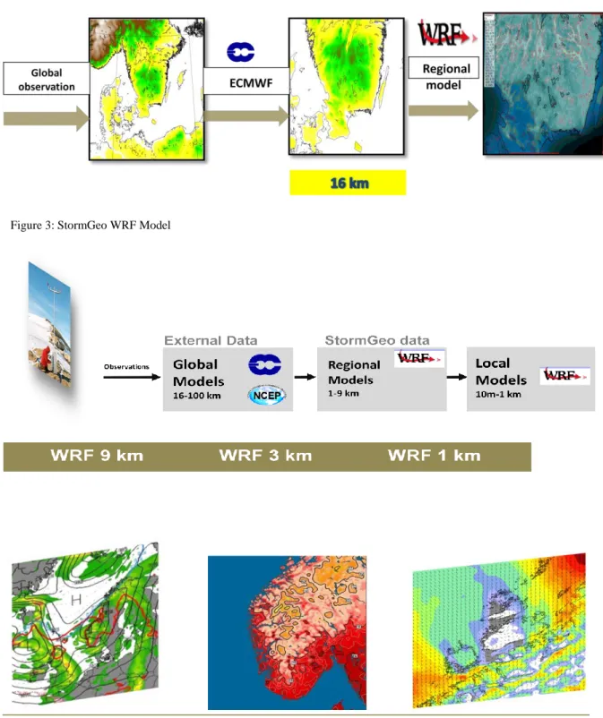
The main forecast model for Europe is 9 km WRF model. The latter model runs twice a day, 6 days ahead, and provides all relevant weather parameters from ground level to the top of the atmosphere. The 9 km WRF model takes in boundary data from the global ECMWF model. see Figure 3.
For detailed, local forecasting, StormGeo runs the WRF and other models in finer resolution over smaller areas, using boundary values from the 9 km model. Thus, for short-term wind power forecasting we run nested models of 9, 3 and 1 km resolution to obtain very detailed, local wind forecasts. The 3 km model uses data from the 9 km model as boundary data, and the 1 km model uses data from the 3 km model as boundary data, see Figure 4. This very fine resolution makes it possible to predict the wind energy generation for each individual wind turbine. [8]
Figure 3: StormGeo WRF Model
The WRF model is also used in hindcast (i.e., historical) mode for resource assessment and sitting purposes. StormGeo has performed numerous studies for the wind farm areas in Scandinavia, using the 1 km WRF with calibration to local measurements, and 6 km for North Sea and surroundingssee Figures 5 and 6.
Figure 5: WRF 6 km area for the North Sea and surroundings Figure 6: Areas in Scandinavia covered with 1 km hindcasts, May 2011
4.2 The ECMWF Model (StormGeo)
To provide boundary data for the WRF model, as well as for forecasting on a global scale, StormGeo uses the so-called ECMWF model, run by the European Meteorological Centre (ECMWF). The ECMWF model is widely recognized as the best performing global weather model in the world. [8]
The model has a horizontal resolution of about 16 km and a maximum forecast length of 10 days. As one of few private weather companies, StormGeo is a member of the ECMWF and
5. Methodology of CFD calculations at mesoscale:
This chapter describes in details how the simulations went through WindSim and how the data series were extracted from the StormGeo`s web based database.
The whole process of ERA Interim data series simulation was fully completed using the WindSim program consisting of 6 modules as shown below, see Figure 7.
Figure 7: WindSim 6 modules
The comparison was made between a met mast data series and the Era Interim (Global Weather Reanalyze Model) both locations are in Maglarp. The aim of the comparison was to see how close the value of the Era Interim to the met mast is (both of the same year of 1989).
5.1 Terrain Module:
The terrain module generates a 3D model of the area around the wind farm based on elevation and roughness data. However, firstly the basis for the 3D model must be available which is a 2D dataset with elevation and roughness data in gws format.
5.1.1 Map:
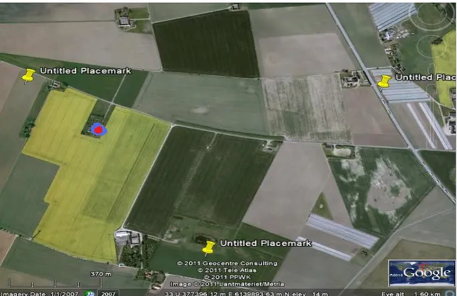
The map was created first by Google earth to get a background for the terrain map which will be used in WindPro/Wasp. This was done by deciding on 3 coordinates in the area around Maglarp in south of Sweden. The location of the site is at Maglarp (coordinates of (SWEREF 99 TM) N=6139758 and E 377268). The area considered plain and with no terrain complexity, see Figure 8. This background map was manipulated in Wasp and has been prepared for implementing the roughness area and height contours. Both roughness area file and height contour file were created by importing the data online. These two files were merged/pasted together into one file and converted to gws format that is adapted to the
WindSim program. The gws file of Maglarp with specific coordinates, roughness area and height contour were used in the terrain module and created the base for the next module.
Figure 8: Location of Maglarp, the red colour is the actual met mast
5.2 Wind Fields Module:
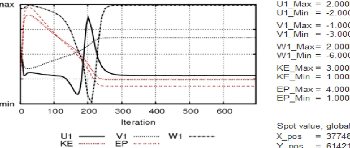
After the generation of the 3D model in the previous Terrain module the simulation of the wind fields can begin. The wind fields are determined by solving the Reynolds Averaged Navier-Stokes Equations (RANS). Since the equations are non-linear, the solution process is iterative; therefore the solution is resolved by iteration until solution reaches a convergence state, see Fig 9 and 10. Since this module is most time consuming; therefore, only some sectors were chosen due to the limited time of this thesis work. The log profile is defined from ground up to the boundary layer height; above this height the profile is constant. Therefore, default value is 500 m. This simulation includes 700 iterations done.
Figure 9: convergence after about 300 iterations, spot value
5.3 Objects:
This module is used to position turbines, climatologies and transferred climatologies. Alternatively objects can also be read from ows files by using the Tools->Import objects menu item. This thesis used the ows format to position both the turbine and the climatology. The turbine was positioned in the ows file just in order to use the energy module and get the wind speed file in wind resources module.
Additionally, this module used the file of both met mast and the ERA interim and uploaded by changing the format that is adapted to windsim as tws or wws format. The tws format is a type of 8 column of the tws windsim format.
5.4 Wind resources:
This module is based on weighting the wind database against measurements. If several measurements are available, the wind resource map will be based on all of them by interpolation. This model is the basis for the energy optimization. In this module the wind speed of the specific coordinate was obtained by a wind resources file after running the wind resources module. Also in this module the shooting for different hub height was obtained and selected with various wind resources file with respective height.
5.6 StormGeo:
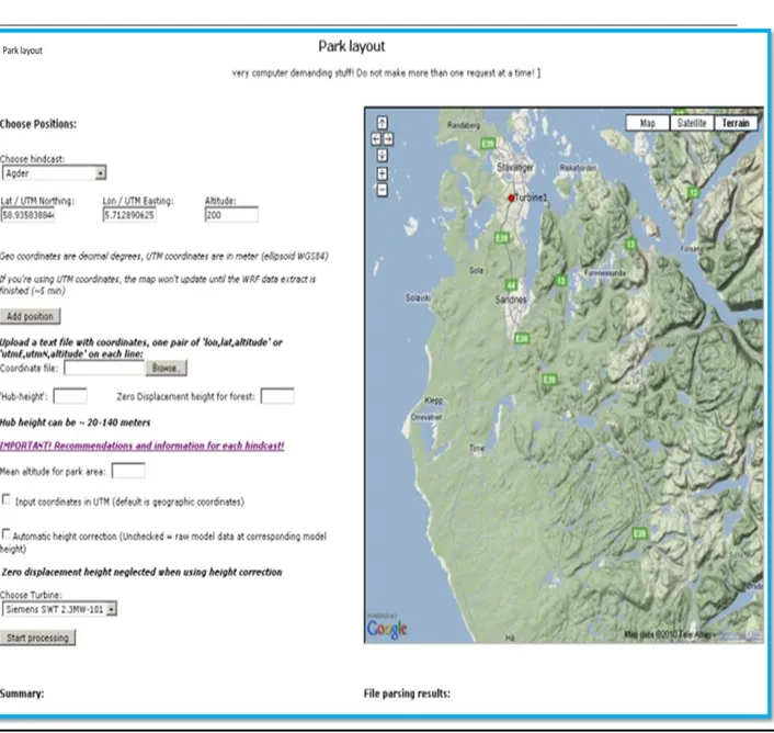
After getting the access (password and user name) from StormGeo company then it was
possible to obtain the ERA interim reanalysis data series for the year 1989 until present. This process is quite easy and simple, see Figure 11. The only thing one must do is to choose the hindcast region, then the coordinates of the Maglarp location with its Zone area number, then the altitude, hub height, and finally clicking on the start processing. After a few minutes of waiting all the data online were obtained, three files were created; first for Era Interim, second file is in Windsim format, third the WRF 1 km resolution of data series for year 2008.
Figure 11: The Stormgeo page for importing data series
6. Results:
After running ERA Interim in WindSim and comparing it with both the ERA Interim raw data and met mast data series, the following results were obtained in the next section.
6.1 Differences in wind speed between two models with initial calculation height of ERA Interim based data on WindSim of 38m:
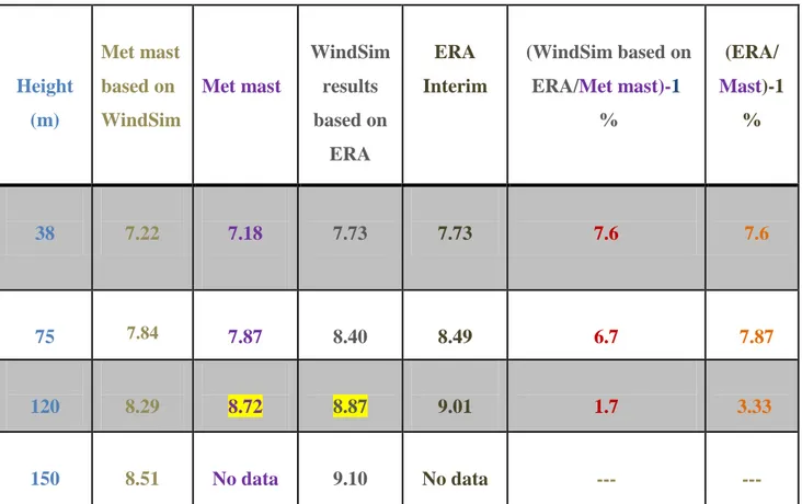
After using the WindSim Model and Global Weather Model (ERA Interim Reanalyze Model) for comparing, the following results were obtained: the measurements of the wind speed for the Maglarp location between the met mast, Era Interim data series and Era Interim based on WindSim with calculations from 38 m height. See Table 1.
The comparison shows that the value between ERA Interim raw data series is very close to the value of the met mast, especially at height of 120m. Furthermore, the Era Interim based on WindSim make the value even much better and closer to the value of the met mast. See Figure 12. Height (m) Met mast based on WindSim Met mast WindSim results based on ERA ERA Interim (WindSim based on
ERA/Met mast)-1
% (ERA/ Mast)-1 % 38 7.22 7.18 7.73 7.73 7.6 7.6 75 7.84 7.87 8.40 8.49 6.7 7.87 120 8.29 8.72 8.87 9.01 1.7 3.33 150 8.51 No data 9.10 No data --- ---
Figure 12 : Computation of ERA Interim based data on WindSim of 38m
6.2 Differences in wind speed between two models with initial calculation of ERA Interim based data on WindSim of 10m:
The comparison, see Table 2, shows that the value between ERA Interim based on WindSim with the met mast value is not accurate since shooting the initial height value is of 10m as the following table shows. See Figure 13.
4 4,2 4,4 4,6 4,8 5 5,2 5,4 5,6 5,8 6 6,2 6,4 6,6 6,8 7 7,2 7,4 7,6 7,8 8 8,2 8,4 8,6 8,8 9 9,2 9,4 0 20 40 60 80 100 120 140 Met Mast ERA
Table2 : Computation of ERA Interim based data on WindSim of 10m
Height Met Mast WindSim results
based on ERA Interim
(WindSim based on ERA/Met Mast )-1
%
10 5.75 7.25 26
38 7.18 8.71 21.3
75 7.87 9.45 20
Fig 13: Computation of ERA Interim based data on WindSim of 10m
6.3 Differences in wind speed between two models with initial calculation of ERA Interim based on WindSim of 75m:
The comparison, see Table 3, shows that the value between ERA Interim based on WindSim with the met mast value have regained its accurate value since calculating the initial height value starts from height of 75m.
4 4,2 4,4 4,6 4,8 5 5,2 5,4 5,6 5,8 6 6,2 6,4 6,6 6,8 7 7,2 7,4 7,6 7,8 8 8,2 8,4 8,6 8,8 9 9,2 9,4 9,6 9,8 10 10,2 10,4 0 20 40 60 80 100 120 140 Met Mast ERA
Table 3: Computation of ERA Interim based data on WindSim of 75m
7. Uncertainty:
Even the met mast value of two different anemometers that are put together at same height and location, gives different values in wind speed per year, according to Daniel Fridriksson from StormGeo, similar measurements have been taken in Norway and showed an average difference of wind speed with 0.5 m/s per year . So differences between the ERA Interim and the met mast with highest 7% are acceptable and lowest 1.7 % is very good.
On other hand all measurements have mechanical and systematical uncertainty with some percent margin error of uncertainty, therefore differences between 2 models is reasonable when the differences are not so high.
Height (m)
Windsim results based on ERA 10m
%
(Met Mast- Windsim based on ERA)-1 %
75 8.40 6.7
8. Discussion:
The ERA Interim and especially ERA Interim based on WindSim has a very close value to the met mast at height such as 100 or 120 m. Therefore, in the area with plain terrain close to the sea in hindcast of Skåne the Era Interim can be used for feasibility study in order to build wind farms.However, Era Interim has not got an accurate value at the height of 50 m and below since the ERA Interim has a low quality and less accurate value at these heights.
The ERA Interim based on WindSim makes the value of the ERA even much better and close to the met mast value if the calculation starts at height of 38 even higher.
9. Conclusion
:It raises the question if it is feasible to use ERA Interim for wind energy assessment, and if these results be generalized in all areas. Building a windfarm with hub height such as 100 or 120 m is feasible with Era Interim with such area like Skåne with no terrain complexity and close to the sea. On other hand it might not be feasible to build wind farm if the wind farm is with low hub height such as hub 50 m and below. This research cannot be generalized in all areas since this thesis work was based on a specific area with a specific topographic character, thus, further research and studies need to be completed in various areas with different terrains in order to get a final conclusion. If this comparison in that hindcast that Era has used efficient it saves money and time.
References:
[1] Sciencedirect, Simultaneous nested modeling from the synoptic scale to the LES scale for wind energy applications, 2011 April 15
<http://www.sciencedirect.com/science/article/pii/S0167610511000158>
[2] WindSim AS, WindSim | Technical Basics, 2011 April 30,
<http://www.windsim.com/product-overview/windsim---technical-basics.aspx>
[3] Wikipedia, European Centre for Medium-Range Weather Forecasts, 2011 May 03,
< http://en.wikipedia.org/wiki/European_Centre_for_Medium-Range_Weather_Forecasts>
[4] ECMWF, Forecasting by computer, 2011 May 05,
<http://www.ecmwf.int/about/overview/fc_by_computer.html>
[5] ECMWF, ERA-Interim, 2011 May 03,
<http://www.ecmwf.int/research/era/do/get/era-interim>
[6] WRF, About the Weather Research & Forecasting Model, 2011 May 08,
<http://www.wrf-model.org/index.php>
[7] Stormgeo, About Stormgeo , 2011 April 08,
< http://www.stormgeo.com/?mapping=8>
[8] Stormgeo, Modellning , 2011 May 12,