Investigation of the magnetic fields of a young Sun-like star ∏1 UMa

UPTEC F 20002

Examensarbete 30 hp

January 2020

Investigation of the magnetic fields of

a young Sun-like star π

_​

1

_​

_UMa

Lawen Ahmedi

Abstract

Investigation of the magnetic fields of a young Sun-like star π

_​

_UMa

In astronomy, the Sun has an important role. It keeps the solar-system together and is the

source for life, heat, light and energy to Earth. As any other star or planet, the Sun has a

magnetic field. The magnetic field of the Sun has a great impact on the Sun itself as well as

its surrounding. The magnetic field shapes solar wind, causes flares and drives coronal mass

ejections radiating towards the Earth (and other planets). The Sun’s magnetic field is still not

fully understood, and therefore it is useful to study other stars with properties similar to the

Sun. So by studying young solar-type stars, the evolution of the Sun can be more easily

understood. The aim of this project is to study the surface magnetic field in a young

solar-type star, π _​1 _{UMa to see how the magnetic field is distributed and if there are any}

patterns like polarity reversals. Magnetic field generates polarisation and with Stokes vector _​I

and _{​V​, polarisation can be described. Earlier measurements from two time-epochs (2014 and}

2015) of Stokes _{​I and ​V have been obtained from the spectropolarimeter NARVAL. To get}

the desired mean polarisation profiles of the star, a technique called least square

deconvolution was applied which increases the signal-to-noise level. To reconstruct the magnetic topology the Zeeman-Doppler imaging technique was used. Then we obtained the

surface magnetic field maps of both measurements. No change of the polarity of magnetic

field at the visible stellar pole was found. Most of the magnetic field energy was contained in

the spherical harmonic modes with angular degrees _{​l​=1-3. The star shows dominance in the}

toroidal component so the study seem to agree with the previously established trend that

younger and faster rotating stars have predominantly toroidal magnetic fields and older stars

with slower rotation rate, like the Sun, have predominantly poloidal field. Looking at the

magnetic field plots, the star show dominance in the azimuthal field component, and the

mean magnetic field strength is similar to one found in the previous study. The results of the

surface magnetic field in our study thus agrees with previous study of the same star. With this

we can conclude that the Sun’s magnetic field probably been different when it was younger,

and possibly similar to the star analyzed in this study.

Handledare: Oleg Kochukhov Ämnesgranskare: Eric Stempels Examinator: Tomas Nyberg ISSN: 1401-5757, UPTEC F 20002

POPULÄRVETENSKAPLIG SAMMANFATTNING

Solen är en viktig del inom astronomin och är källan till värme, ljus och liv på jorden. Likt

andra planeter och stjärnor har solen ett magnetfält som har en stor inverkan på solen och

dess omgivning. Från solens magnetfält bildas bland annat starka solvindar och emitterar

partiklar som åker mot jorden och andra planeter. Aktiviteten hos solen varierar regelbundet i

en 11-årscykel då magnetfältet byter polaritet. Men än idag finns fler oklarheter kring hur

solens magnetfält utvecklats från sitt yngre stadie då solen var flera miljoner år yngre. Ett sätt

att analysera solens utveckling och magnetfält på är genom att studera andra stjärnor som har

liknande egenskaper som solen men som är flera miljoner år yngre. I denna studie har den

300 Myr gamla stjärnan π _​1_{UMas magnetfält studerats. Med hjälp av analytiska metoder, som}

Zeeman Doppler Imaging (ZDI) är det möjligt att rekonstruera stjärnans polariseringsprofiler

till kartor över magnetfältet på ytan. Med Stokes vektorer I och _{​V är det möjligt att beskriva}

dessa polariseringsprofiler, som givits från två olika mätningar tagna 2014 respektive 2015 från spektropolarimetern NARVAL. För att beräkna polariseringsprofilerna applicerades tekniken “least square deconvolution analysis” som höjer signal-brusnivån, och därefter

användes ZDI-metoden för att rekonstruera magnetfältet, vilket resulterade i mappar på

magnetfältets distribution på stjärnans yta. Stjärnans magnetfält visar dominans hos toroidala

magnetfältet samt ett starkare fältstyrka i azimutala komponenten. Vid jämförelse med en

tidigare studie [7] av samma stjärna som använt mätningar från 2007 verkar resultatet överensstämma och det verkar som att stjärnan har hållit samma magnetiska aktivitetsnivå mellan dessa två epoker. Ingen förändring hos stjärnans polaritet kunde påvisas, men

eftersom mätningarna i denna studie var tätt inpå varandra (6 månader emellan) och stjärnan

haft samma polaritet år 2007 från förra studien, är det troligt att skiftningen hos polariteten

missats om det nu skett. Med detta kan vi konstatera att solens magnetfält möjligtvis sett

annorlunda ut när den varit yngre, och möjligtvis likt stjärnan som analyserats i denna studie.

Abstract 2 POPULÄRVETENSKAPLIG SAMMANFATTNING 3 1.Introduction 5 2.Theoretical background 7 2.1 Magnetic fields 7 2.2 Polarisation 8

2.3 Stokes parameter spectra 9

2.4 Mapping of stellar magnetic fields 10

2.5 π_​1​ _{UMa 12}

3. Method 12

3.1 Observational data 12

3.2 Least squares deconvolution analysis 13

3.3 Zeeman Doppler Imaging 14

4.Results 16

4.1 Observed LSD profiles 16

4.2 Reconstructed magnetic field maps 20

5. Summary and discussion 28

6.References 30

1.Introduction

Stars are fascinating objects covering the sky. The Sun is a star in our Galaxy, the Milky Way

planetary atmospheres. The magnetic field of the Sun has a great impact on the Sun itself as

well as its surrounding, for example the Earth. The magnetic field shapes solar wind, causes

flares and drives coronal mass ejections radiating towards the Earth (and other planets),

which are storms consisting of high-energy particles. The Earth has a magnetic field that is

partly protecting it from the Sun’s magnetic activity by deflecting the particles from the solar

wind. But still, the most powerful eruptions are affecting us since they affect the outer layers

of the terrestrial atmosphere, can harm electronics, the satellites in outer space, and could also

be harmful for the astronauts. Thus, the solar magnetic activity has an important role. The

Sun’s magnetic field is still not yet fully understood, and therefore it is useful to study other

stars, for example Sun-like stars of younger ages, to understand long-term evolution of the

solar magnetic activity. The focus in this project will be on such young solar-type star, UMa.

π1

Solar-type stars are defined as objects within the mass range 0.6M _​⊙_​≤M≤1.5M​⊙_​, where M​⊙_​is

the mass of the Sun. These stars belong to the spectral classes from mid-F to late-K. They

have similar pattern of “magnetic activity”, believed to be the outcome of the dynamo

process operating in the stellar interiors. The presence of the field at the stellar surface is

revealed by several types of indirect activity proxies, such as cool starspots, X-ray emission

or enhanced emission in the chromospheric lines. Solar-type stars are born rapid rotators. The

rapid rotation makes the generation of magnetic field more efficient, and therefore young

and/or rapidly rotating stars are more active and have therefore stronger fields and the

magnetic spots are larger on their surfaces. Magnetic fields of most of the solar-type active

stars have a strong azimuthal component usually arranged in azimuthal rings on the stellar

surface[3]. With age, the stars will become slower rotators and their magnetic activity will

decrease. The Sun rotated much faster when it was younger because the stellar rotation is

slowed down by the magnetic field, which also implies that the magnetic activity was higher.

Previous studies have suggested that the level of activity of cool stars decreases with age and

therefore the Sun is currently different from its younger state[7]. The aim of this project is to

study the magnetic field of a young solar-analogue star to gain more knowledge about stellar

magnetism in the context of understanding the history of the Sun and its magnetic activity.

Understanding the Sun’s activity history would also enhance our knowledge of the effect of

the activity of the Sun on earlier atmospheres of the terrestrial planets such as Earth and

Mars. Earlier studies have shown that the Earth in its younger stages have always had liquid

water, which must indicate that its surface was warmer than could be sustained by fainter

young Sun. Probably Earth was heated by greenhouse gases such as methane and carbon

dioxide.​Previous observations of Mars have shown convincible signs of liquid water on its

surface, which means that its atmosphere has been more compact and warmer at earlier

evolutionary stages[2]. These are some examples of what information investigation of stellar

magnetism of solar-analogue stars can provide us, which is a part of the purpose of this study.

It is also interesting to study the pattern of magnetic polarity reversal, which is a change of

field over different time-periods, the polarity reversal can be observed. For example, the Sun

has a 11-year cycle where the Sun’s magnetic field reverses polarity[15]. Also, in reference

[7] one has studied several different Sun-like stars and a polarity reversal have been seen for

one of the stars ( _​χ​1 _{Ori) with a periodical cycle of either 2,6 or 8 years, which might suggest}

that the Sun had a different cycle when it was younger.

Magnetic field generation is an important process in stars. Due to magnetic fields dark spots

are formed at the surface of the Sun. These dark spots cause variability, flares and

short-wavelength emission that affects the immediate stellar environment and the entire

planetary system. It is possible to study magnetic fields and spots of stars other than the Sun

using computer tomography techniques to convert time variability of polarisation profiles of

stellar spectral lines into two-dimensional maps of spots and vector magnetic fields on the

stellar surface. In this project, an analysis of the young star named π1UMa, which is similar

to what our Sun was a few hundred million years after its formation, will be performed using

previously collected observations, obtained 2014 and 2015. The analysis begins with

detecting a weak polarisation signal (which is a direct signature of magnetic field) in stellar

spectral lines by applying multi-line analysis technique. The study is performed with

computer codes written in IDL and Fortran. The detected signal will be modeled with a

tomographic code and the magnetic fields will be reconstructed followed by an analysis of

the obtained results. This surface magnetic field mapping will be performed using

Zeeman-Doppler imaging (ZDI) analysis of Stokes _{​I and ​V spectropolarimetric observations}

with a code developed by [3]. We aim to obtain maps of the magnetic field at the stellar

surface. This allows us to study the magnetic field distribution of the star in detail for two

different sets of observations obtained with the NARVAL spectropolarimeter in 2014 and

2015 and investigate how the field change over time. Also a comparison with the results of

the study from reference [7] will be carried out, where the magnetic field of π1UMa was

studied using observations from 2007. This project will hopefully improve our understanding

of the magnetic field of π _​1 _{UMa in particular and magnetism of young Sun-like stars in}

general.

2.Theoretical background

2.1 Magnetic fields

In stars, magnetic fields have an important role during many stages of stellar formation and

evolution. The motion of the conductive plasma in a stellar interior creates magnetic fields.

The magnetic energy is derived from the kinetic energy of stellar rotation and convection.

Interaction between the magnetic field and stellar wind is the main mechanism of angular

momentum loss in young stars. Magnetic fields produces phenomena such as star spots,

The presence of a magnetic field leads to changes in the atomic energy levels resulting in

changes of the properties of spectral lines. The magnetic field splits spectral lines in a number

of components and introduces circular and linear polarisation within these components. These effects make it possible to detect stellar magnetic fields.

In a magnetic field, the atomic Hamiltonian is given by

H =− ħ ∇ (r) (r)L (L S) (B ) (1) 2m 2_{+ V + ξ · S +} eħ 2mc + 2 · B + e 2 8mc2 × r 2

where _{​m and ​e correspond to the electron mass and charge, ​c ​and ​ħ ​are the speed of light and}

the Planck constant respectively, _{​L ​and ​S are the orbital and spin angular momentum}

operators and _{​B ​corresponds to the magnetic field vector. Three different regions are defined}

depending on the relative strength of the spin-orbit interaction and the magnetic field terms.

The linear Zeeman effect occurs when the quadratic field term is smaller than the linear field

term which in turn is smaller than the spin-orbit term. The Paschen-Back effect occurs if the

quadratic field term and the spin-orbit term are smaller than the linear field term. The

quadratic Zeeman effect occurs when the quadratic field term is larger than the linear field

term and larger than the spin-orbit term.

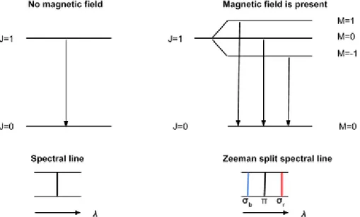
Figure 1. Representation of atomic energy levels and corresponding spectral lines when there

is no magnetic field in comparison to the case when a magnetic field is present.

In figure (1) we can see an illustration of the typical effect of magnetic field on a spectral

line. Without magnetic field, the transition between the upper and lower atomic levels gives

rise to a single spectral line. When a magnetic field is present the line splits into three groups

of Zeeman components (σ_b, π, σ ) r [3]. Figure (1) shows the simplest type of splitting

2.2 Polarisation

Electromagnetic waves have a property to oscillate in a certain way, which is called

polarisation. If the direction of the electric field vector within the electromagnetic wave ​varies

randomly in time the light is said to be unpolarized. A non-random behaviour of the ​electric

field determines what type of polarisation is present in electromagnetic wave. _​Linear

polarisation is a plane electromagnetic wave, i.e the electric field vector is moving in a single

plane along the direction of propagation. Circular polarisation is when the electric field vector

rotates in a circle, i.e the electric field in the wave has two orthogonal linear components

which are equal in amplitude and vary with a phase shift of /2π . Elliptical polarisation is

when the light consists of two perpendicular components with any amplitude and shift [3]. The Stokes vector describes the polarisation of an electromagnetic wave and it is given by:

_{I = {I, , , }Q U V} T ​ _{​ (2)}

Each term is defined as: Stokes _{​I - Total intensity of radiation, which is equal to the sum of two beams with} orthogonal polarisation, i.e I = I₀+ I₉₀ = I₄₅+ I₁₃₅ = I_↻+ I_↺. (3)

Stokes _{​Q​ - Difference in the intensity of} Q = I₀− I₉₀. (4)

Stokes _{​U​ - Difference in the intensity of} U = I₄₅− I₁₃₅. (5)

Stokes _{​V​ - Difference in the intensity of} V = I_↻− I_↺. (6)

where (3) corresponds to unpolarised light, (4) and (5) describes linear polarisation and (6)

Figure 2. An illustrations of the properties for polarisation of the radiation that is emitted in

the Zeeman components ( and ) for different orientations of the magnetic field vectorπ σ

relative to the line of sight.

The Zeeman components in the split spectral line have distinct polarisation properties. The

polarisation depends on the angle between the magnetic field vector and the direction of the

emitted light, and changes according to that, as can be seen in figure (2).

When light emitted is parallel to the field vector, the π components disappears and the σ _​band

σ_​rcomponents have opposite circular polarisation. If the line of sight is perpendicular to the

field vector, the π components are linearly polarised parallel to the field and the σ _​b and σ _​r

components are linearly polarised perpendicular to the field. This means that the π

components can only be linearly polarised and the σ components can have both circular and

linear polarisation[3].

Due to weakness of surface magnetic fields in stars it is usually challenging to detect them

directly. Nevertheless, it is possible to study and detect these fields using polarisation in

spectral lines. This will be presented in section 2.4.

2.3 Stokes parameter spectra

To interpret polarisation spectra of stars we need to know how to theoretically compute

shapes of spectral lines in four Stokes parameters. This is accomplished by solving the

radiative transfer equation in the thin outer layer of the star - the atmosphere. This equation

describes the interaction between matter and radiation. When a magnetic field is present, a

single scalar equation for the intensity is replaced by the analogous transfer equation for the

Stokes _{​I​ vector as following:}

_dzdI _{= K + J}− I (7)

where z is the height in the stellar atmosphere, I = {I, , , }Q U V T is the Stokes vector. The

parameter K is a matrix which describes the absorption of light and attenuation of its

polarisation characteristics and J is the emission vector. In order to solve the polarised

radiative transfer (PRT) equation several input parameters are required, listed below:

- the magnetic field vector _{​B​ as a function of z,}

- the temperature and pressure as a function of z,

- the data of relative concentrations of chemical elements whose lines we want to

model

- a database that contains information about the continuum opacity coefficients of

relevant absorbers, and a line list with information about the position of spectral lines,

their transition probabilities, broadening parameters and parameters J_u,l and g_u,l

needed in order to compute the Zeeman splitting patterns

With all of these input parameters applied, one can numerically solve the PRT equation

obtaining the Stokes vector _{​I as a function of wavelength for each layer in the stellar}

Another way of solving the PRT equation with less complication than the previous one, is to make use of approximate analytical solutions. One such solution corresponds to the

Milne-Eddington (ME) atmosphere, which assumes that the magnetic field, the ratio of the

line and continuum opacity as well as the absorption and anomalous dispersion profiles

which enter the matrix K are all constant in the line formation region, and that the source

function (which enters the definition of the emission vector J) is linearly dependent on the

optical depth .τ

The preceding discussion concerned the problem of calculating the local Stokes vector from

local properties. But studying stellar magnetic fields is more complex. Stars are unresolved

objects, and the magnetic field vector changes from one region to another on the surface.

Every surface zone creates its own Stokes vector. Because of stellar rotation these local

Stokes vectors are ​Doppler-shifted and weighted according to the local brightness and

projected surface area. The contribution of the surface zones on the stellar hemisphere and

adding them all together produces disk integrated Stokes profiles_​, which approximates the

real observations of stars. These disk integrated profiles are time-dependent since the star is

rotating and we are observing the field structure from different angles.

2.4 Mapping of stellar magnetic fields

The main tools for investigating stellar magnetic fields and surface structures are high-resolution spectroscopy and spectropolarimetry. The spectral line profile shapes are

distorted due to inhomogeneities on stellar surface, which create detectable signatures in the

line profiles. As described above, magnetic field generates polarisation in spectral lines

through the Zeeman effect. This allows detection of stellar magnetic fields and reconstruction

of their topologies. To accomplish the latter task, spectropolarimetric observations have to be

obtained several times to resolve rotational modulation.

Reconstruction of two-dimensional maps of stellar surface is carried out using Doppler

imaging (DI) and Magnetic/Zeeman Doppler imaging (MDI/ZDI), which are the highest

resolution indirect imaging methods in astronomy. _​These techniques use the fact that

distortions generated by magnetic fields and star spots move across Doppler-broadened

intensity and polarisation line profiles. Any point in the line profile represents an interval of

Doppler shifts corresponding to a vertical stripe on the stellar surface. Features in a single

Stokes profile can be used to determine longitudinal position of a magnetic or cool spot on

the stellar surface. The latitudinal information can be obtained from a times series of Stokes

profiles recorded at different rotational phases. For example, if the star has an inhomogeneity

at the surface near the pole, its line signature is visible only near the centre of the profile and

persists during more than half of the rotation period. On the other hand, a spot near the

equator travels through the whole profile and is visible during only half of the rotation cycle.

be reconstructed. The magnetic field topology can be reconstructed using the same principle

applied to polarised spectra, and this technique is known as Zeeman Doppler Imaging.

Starting from some input parameters (brightness, magnetic field, temperature, chemical

abundance) and by using a times series of the line profiles, a reconstruction of a

two-dimensional map of the stellar surface can be accomplished. DI is mathematically an

ill-posed problem, meaning that infinite number of solutions can fit a given set of

observations. DI needs an additional constraint in order to have an unique solution, which is

called regularization.[3]

Zeeman Doppler Imaging (ZDI) or the inverse method, is the only technique for

reconstructing stellar magnetic field topologies with the ability to extract a quantitative

information about stellar magnetic field for stars with complex fields[3]. Since many stars are

too far away from the observer, the technique uses the rotation of the star to reconstruct the

magnetic field distribution at the surface of the star.

Doppler Imaging is most efficient for fast rotating stars but can also be applied for slow

rotating stars. It is not optimal to use only circular polarisation. Only information about the

line of sight component of the magnetic field vector can be obtained from Stokes _{​V since it is}

independent of the azimuth angle. For that reason the same Stokes _{​V profile can represent}

different field configurations [7]. However, in practice, recordings of the Stokes _{​Q and ​U}

spectra are very difficult to obtain because they have about 10 times smaller amplitude than

the Stokes _{​V​ signal. In this study we rely only on Stokes ​V​.}

2.5 π

_​

​

UMa

The young solar-analogue star π _​1 _{UMa is considered to be a member of the Ursa Major}

Moving Group, which includes a group of stars that has the same velocity vectors in space

and is believed to have a common origin in space and time. All of the stars belonging to this

group have an age of about 300 Myr[7]. In comparison, the Sun has an age of 4.6 Gyr. We

will compare our results with reference [7] who also studied the star π_​1​ _UMa.

3. Method

3.1 Observational data

In order to perform magnetic field analysis of the star π 1UMa two sets of previously

observed data are used. The first set of observed data is taken April 2014 and the second set

of data is taken January 2015. _​The first dataset contains 14 observations. The observations are

taken with short intervals, typically 1-2 days, and some have been taken the same night at

different times. The second dataset consists of 12 observations with a 1-day interval and two

The reduced spectra have been taken from a database called PolarBase. PolarBase is a database which contains all stellar data that has been obtained with the high-resolution

spectropolarimeters ESPaDOnS and NARVAL, in their reduced form[4]. NARVAL is one of

the few astronomical facilities around the world fully dedicated to stellar spectroscopy,

located in Pic du Midi, France. It is installed at Télescope Bernand Lyot and is a “twin” of the

spectropolarimeter ESPaDOnS installed at the Canada-France-Hawaii Telescope (CFHT;

Mauna Kea Observatory). NARVAL permits long-term surveillance and investigation of

brighter targets. It gives the opportunity to have coordinated observations with ESPaDOnS in

order to achieve a continuous surveillance of rotating and variable stars, which is possible

due to the 160° shift in longitude between Hawaii and France[1]. The spectrograph NARVAL

has a polarimetric unit consisting of three Fresnel rhombs. This device allows one to obtain

circular polarisation spectra or spectra in all four Stokes parameters. In order to prevent

spurious polarisation and to decrease the number of reflections before light passes into the

spectrograph, the polarimetric unit is installed at the Cassegrain focus. The resolving power

of NARVAL is around 65 000 and the spectrograph covers the wavelength range from 3700

to 10 500 Å, which corresponds to the entire optical spectrum. The reduced spectral files

include, in addition to Stokes _{​I and ​V​, the so-called “null” spectrum, which should only}

contain background noise created by suppressing the true stellar polarisation. The “null”

spectrum is included from the data files which were downloaded from the Polarbase archive.

In polarimetric mode, when a spectrum is produced, four subexposures are combined with the

polarimetric optics rotated by varying the angle on the optical axis. By adding together the

four subexposures, corresponding spectrum for Stokes _{​I is obtained. Taking other}

combinations of the subexposures makes it possible to obtain the “null” spectra[4]. This

spectrum is useful for assessing instrumental artefacts and noise in the data. The

measurements analysed here were obtained only with NARVAL, a stellar spectropolarimeter,

duplicated from the spectropolarimeter ESPaDOnS.

3.2 Least squares deconvolution analysis

The star analysed here has a has relatively weak magnetic field. _​Weak magnetic fields are

hard to detect, because they produce weak polarization signatures in individual lines. By

using the LSD (least squares deconvolution) method it is possible to detect weak polarisation

signals by increasing the signal-to-noise (S/N) level. The LSD technique adds together all

lines in a spectrum into a single intensity profile. The same principle is applied to the

corresponding polarization profiles, instead of studying them in individual lines. The LSD

analysis is developed by [9] and is a method of extracting highly precise mean Stokes _​V

signatures from polarisation observations with a moderate S/N. This technique was extended

to all four Stokes parameters by [10]. LSD represents the entire stellar spectrum as a linear

superposition of scaled mean profiles. Mathematically it can be described as:

X = M · Z_X (8) where _{​M is the line pattern matrix and ​Z​ X​is the mean profile which is sought for, and ​X=X​ ob​s}

The least squares problem of fitting the model given by equation (8) to observations is given by

χ2 _{= (}X ) (X ) > min (9)

obs− M · ZX T · E2obs obs− M · ZX −

and its solution is following

Z_X = (MT · E2_obs· M)−1_{* M}T · E2_obs· X_obs, (10)

here E_obsis the diagonal matrix consisting of the inverse of the error bars, 1/σ_obs[3].

The purpose of the LSD analysis is to solve the inverse problem of equation (8), which means

obtaining the mean line profile _{​Z ​for a given pattern matrix ​M​ and observed spectrum ​X​obs​}.

During this step the observed mean line profiles of Stokes _{​I and ​V​, the corresponding errors}

and the “null” spectra for all observations of π _​1 _{UMa spectrum are going to be obtained. The}

stellar parameters used for compiling the list of lines for LSD are the effective temperature

and the surface gravity _​[7].

875 K

T_eff = 5 log(g)= 4.49 cm/s 2

For the LSD analysis a code has been developed by [8]. From the Vienna Atomic Line

Database [13] we received a line list for the stellar parameters given above. The starting

wavelength used was 3900 Å and ending wavelength 10000 Å. The microturbulence is set to

(typical value for Sun-like stars) and the line-depth selection threshold to 0.01_​,

km/s

ξ_t= 1

meaning that only lines deeper than 1% of the continuum were included in the list.

As a simple measure of magnetic field strength, we analysed the mean longitudinal magnetic

field, B_​z​. Following reference [14] it is calculated from the Stokes _{​I​ and ​V​ profiles with}

Bz = 7− 14 [G] (11) V (v)dz

∫v

λg [1−I(v)]dv∫

where _{​λ [µm] is the mean wavelength of LSD line mask and g is the mean effective Landé}

factor, _{​v [km/s] is the velocity shift with respect to the center. The mean longitudinal}

magnetic field corresponds to the disk-averaged line of sight magnetic field component. It is

not sensitive to small-scale fields [5]. It is possible that the integral from the equation (11)

becomes zero, even if there is a magnetic signature in the Stokes _{​V profile. Such symmetry in}

the profile indicates that both sides of the star have magnetic structures of the same strength

but opposite polarities. An example of such configuration is a ring of azimuthal field

encircling the star. Thus, the longitudinal field depends on the magnetic field strength and its

configuration.

3.3 Zeeman Doppler Imaging

The analysis begins with the forward calculation, performed with some input parameters

including the stellar parameters, the line data and magnetic field vectors B ,( _r B_θ,B_a), of the

local Stokes parameters. Then surface integration is carried out, and the appropriate Doppler

sin i and location of a given surface element. _{​The local profile is then multiplied by a weight}

which is the product of the projected surface area of this surface element and limb-darkening

function. The limb-darkening function accounts for the fact that the stellar surface brightness

decreases from the center of the stellar disk to the limb. Afterwards the local Stokes profiles

obtained in previous steps are summed up resulting in the disk-integrated model Stokes

profiles. Then these spectra are compared to the observed data at each rotational phase. Based

on this comparison, the ZDI code adjusts the surface magnetic field distribution, recalculates the model disk-integrated profiles and compares them with observation again. This process

continues until a good fit to observations is achieved. In parallel, the code calculates

regularisation function and tries to ensure that solutions that it converges to also satisfy the

regularisation constraint.

When modelling the LSD profiles we assume that they behave similar to a single spectral line

with average line parameters. By solving the polarised radiative equation using the Milne-Eddington approximation, the local model Stokes profiles were calculated. We obtained the central wavelength and the effective Landé factor from the LSD line mask. The

line shape was parameterized by a combination of a depth parameter (the line depth; the

parameter regulating the strength of Stokes _{​I line in the model that we fit to LSD profiles)}

and a Voigt function described by the two broadening parameters. The final stellar

parameters that are necessary for ZDI analysis are the stellar radial velocity _​v​rad_​, rotational

period _{​P​rot​}, the projected rotational velocity _{​v ​sin i and the inclination angle ​i of the stellar} rotational axis. The initial values of these parameters, _{​v​rad​}=12.35 km/s,_{​i​=60 degrees, ​P​ro​t​}=4.9 d and _{​v ​sin i​=11.2 km/s, were adopted from [7]. ​P​rot}and _{​v​sin i ​are further optimised below to}

obtain better fit to the observational analysed here. The limb darkening is treated according to

a linear function law, with the coefficient 0.65 taken from [6].

The radial, azimuthal and meridional magnetic field components are described with the spherical harmonic expansion:

Br(θ, ) −φ = ∑ Y (θ, ) (12) lmax l=1 ∑l m=−l α_{l,m l,m} φ Bm(θ, ) −φ = ∑ [β Z (θ, ) X (θ, )] (13) lmax l=1 ∑l m=−l l,m l,m φ + γ_{l,m l,m} φ Ba(θ, ) −φ = ∑ [β X (θ, ) Z (θ, )] (14) lmax l=1 ∑l m=−1 l,m l,m φ − γ_{l,m l,m} φ where Y_l,m(θ, ) −φ = C_l,mP_l,|m|(cosθ)K (φ)m , (15) Z_l,m(θ, )φ = C_l+1l,m K (φ) (16) ∂θ ∂P_l,|m|(cosθ) m X_l,m(θ, ) −φ = C_l+1l,m mK (φ) (17) sinθ P_l,|m|(cosθ) −m

are the real spherical harmonic functions describing the mode with the angular degree _{​l and}

azimuthal order _​m

C_l,m=

√

(l−|m|)! and

(19)

where _{​θ and ​ф ​are the longitude and co-latitude angles at the stellar surface. ​P​ l,m​}(θ) _{​is the}

associated Legendre polynomial. The regularisation function applied to the magnetic field

will reduce unnecessary contribution of higher-order harmonic

(α )

R = ∑ l,ml

2 2

l,m+ β2l,m+ γ2l,m

modes. The parameters α_l,m, β_l,m, γ_l,m characterise the contributions of the radial, poloidal,

horizontal poloidal and horizontal toroidal magnetic field components. These harmonic coefficients alpha, beta, gamma are the actual free parameters optimised by the ZDI code.

The expansion is carried out to a sufficiently large l_max. In this study we used l_max = 10[7].

4.Results

4.1 Observed LSD profiles

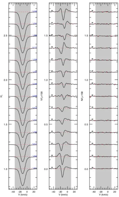
Figure (3) and (4) are plots of the observed LSD Stokes _{​I​ and ​V​ profiles for each dataset}

presented with the “null” spectrum, which characterises noise and false signals. These

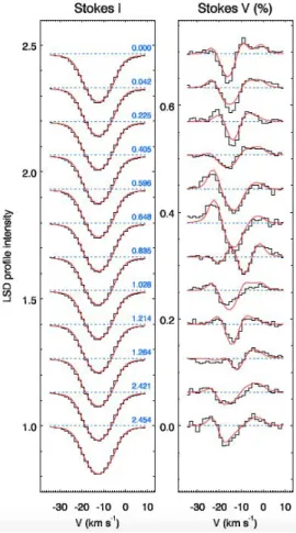
Figure 3. Observed LSD profiles Stokes ​I​, Stokes ​V and “null” respectively, taken in April 2014 scaled with a factor 158. The intensity is shown on the y-axis and the velocity on the x-axis. Rotational phase is marked in blue. The profiles are offset vertically for display purposes. The grey rectangles in the figure represent the intervals within which the statistics and B​z​ are calculated.

Figure 4. Observed LSD profiles Stokes _{​I​, Stokes ​V and “null” respectively, taken in January 2015, scaled with a} factor 170. The intensity is shown on the y-axis and the rotational velocity on the x-axis. Rotational phase is marked in blue. The profiles are offset vertically for display purposes.

One of the important parameters of LSD profile is the cut-off value, which determines how

many lines to include when constructing LSD profile. 5% cut-off means that all lines deeper

than 5% of the continuum are included, 10% means that all lines deeper than 10% of the

continuum are included, etc. The larger the cut-off, the fewer lines are retained in the list,

which can be seen in the last row of table (1). In principle, the more lines we include - the

better. But one can also worry that including many weak lines will degrade the quality of the

mean profile. This is why one of the steps of our analysis was to test S/N of LSD profile as a function of cut-off. In order to try to improve the quality in our calculations, an analysis of

the cut-off value was performed to see if any change in this parameter would give any

determined by the ratio, of the maximum absolute Stokes _{​V amplitude and the mean error of}

Stokes _{​V profile, Q=Max(V)/Err(V). The higher this ratio, the better is the LSD profile}

quality. The total number of lines decreases as the cut-off is increases. One can not see any

significant difference when comparing the quality factors. We concluded that changing

cut-off has an insignificant effect on the results. We have chosen to use the cut-off 20 %

throughout the whole project.

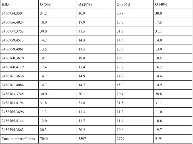
Table 1. Table of quality factors ​Q for different cut-offs (%) for the observed data from April 2014. The last row shows the total number of lines for each cut-off.

HJD Q (5%) Q (20%) Q (30%) Q (40%) 2456754.3504 31.2 30.9 30.8 30.0 2456756.4024 18.0 17.9 17.7 17.5 2456757.3753 30.0 31.5 31.2 31.1 2456759.4513 14.2 14.3 14.5 14.0 2456759.4961 13.5 13.5 13.5 13.0 2456760.3670 19.7 19.8 19.0 18.5 2456760.4119 17.4 17.4 17.2 16.2 2456761.3636 14.7 14.9 14.9 14.4 2456761.4084 14.7 14.7 15.0 14.9 2456763.3745 30.0 30.1 29.4 28.8 2456763.4194 31.8 31.8 31.5 31.1 2456765.3696 11.3 11.3 11.2 11.0 2456765.4144 12.0 11.7 11.4 10.6 2456794.3862 20.3 20.2 19.6 19.7 Total number of lines 7040 3597 2779 2191

The observations from April 2014 and January 2015 are summarised in tables (2ab). The

mean error of Stokes _{​V in the first dataset is smaller than for the second dataset. The error is}

of order 10_​-5​_{in both observations and is typically around 1.9*10 ​}-5 _{in table (2a) and around}

3.5*10_​-5 _{in table (2b). The maximum amplitude is of order 10 ​}-5 ​_{in both observations and}

differs slightly in both sets. The maximum amplitude reaches 6.1*10 _​-4​_{in the first dataset and}

5.6*10_​-4 _{for the second dataset. The longitudinal field B​}

z varies for both datasets, changing

sign, which indicates that the magnetic field topology is relatively complex and definitely not

axisymmetric. B_​z is mostly negative for both datasets with the highest value 0.88 G and

smallest value -10.83 G in the first set, in the second set the highest value is 11.62 G and the

Table 2a. Data from the dataset obtained in April 2014. The table gives heliocentric Julian date, error of Stokes V​, maximum amplitude (by absolute value) of Stokes ​V LSD profile and the longitudinal field ​B​ z​in Gauss and

the uncertainty. HJD Err(V) Max(V) B​z​(V) [G] 2456754.3504 1.921E-05 5.945E-04 -2.34±0.68 2456756.4024 1.324E-05 2.374E-04 -5.97±0.47 2456757.3753 1.426E-05 4.491E-04 -7.40±0.51 2456759.4513 2.281E-05 3.257E-04 -2.58±0.82 2456759.4961 2.053E-05 3.778E-04 -2.75±0.74 2456760.3670 1.905E-05 3.766E-04 0.64±0.69 2456760.4119 1.932E-05 3.364E-04 0.88±0.70 2456761.3636 1.862E-05 2.779E-04 -7.08±0.67 2456761.4084 1.875E-05 2.764E-04 -6.69±0.67 2456763.3745 1.931E-05 5.815E-04 -0.22±0.69 2456763.4194 1.926E-05 6.126E-04 -1.21±0.69 2456765.3696 2.076E-05 2.354E-04 0.01±0.75 2456765.4144 2.067E-05 2.428E-04 -0.19±0.74 2456794.3862 1.983E-05 3.998E-04 -10.83±0.72

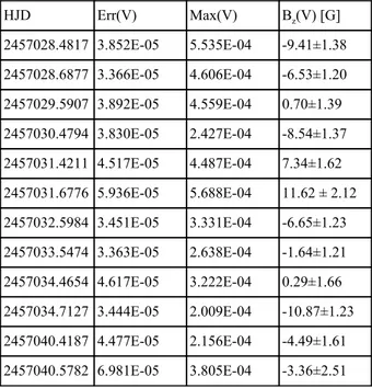
Table 2b. Same as 2a but for the dataset obtained in January 2015.

HJD Err(V) Max(V) B​z​(V) [G] 2457028.4817 3.852E-05 5.535E-04 -9.41±1.38 2457028.6877 3.366E-05 4.606E-04 -6.53±1.20 2457029.5907 3.892E-05 4.559E-04 0.70±1.39 2457030.4794 3.830E-05 2.427E-04 -8.54±1.37 2457031.4211 4.517E-05 4.487E-04 7.34±1.62 2457031.6776 5.936E-05 5.688E-04 11.62 ± 2.12 2457032.5984 3.451E-05 3.331E-04 -6.65±1.23 2457033.5474 3.363E-05 2.638E-04 -1.64±1.21 2457034.4654 4.617E-05 3.222E-04 0.29±1.66 2457034.7127 3.444E-05 2.009E-04 -10.87±1.23 2457040.4187 4.477E-05 2.156E-04 -4.49±1.61 2457040.5782 6.981E-05 3.805E-04 -3.36±2.51

4.2 Reconstructed magnetic field maps

Before modelling Stokes _{​V profiles we need to adjust relevant parameters to reproduce}

Stokes _{​I profile as good as possible. We adjusted two parameters, the line depth and ​v sin ​i.}

The lowest deviation for Stokes _{​I (0.33547 %) we could obtain corresponded to ​v sin ​i} = 10.6

As mentioned previously, regularisation is an important ingredient of ZDI. We start by

exploring impact of different choices of regularisation on the quality of fits to observational

data. Figure (5) shows the fit quality (mean standard deviation of (V/Ic) in %) for 13 different

values of the regularization parameter. The goal is to obtain a simple map with an acceptable

fit. The plot represents which deviation Stokes _{​V was obtained for inversions with different}

regularisation parameters. The deviation decreases with a decreasing value of the

regularisation parameter, so for lower values of the regularization parameter, better results are

obtained. The optimal value for regularization roughly corresponds to where the largest

change of slope occurs in Fig. 5, i.e. around log Λ=-10.

Figure 5. The deviation of Stokes _{​V (in %) is plotted as a function of value of regularization parameter. From the} slope it is possible to determine the optimal value for the regularization. The deviation of Stokes _{​V is decreasing} when the value of regularization parameter is decreasing.

The stellar rotational period is another critical parameter. The initial value used for the

rotational period of the star was _{​P​rot​}=4.9 d. _{​We reconsidered this value since it may not be}

exact, to get a better fit for Stokes _{​V profiles corresponding to the 2014 dataset. Changing ​P​ rot} several times suggests _{​P​rot​}=4.93 d. _{​The mean deviation for the initial value of ​P​ rot​}=4.9 d was

0.00409% and for the adjusted value it changed to 0.00360%. In figure (6) it can be seen that

Figure (6). Plot of the deviation of Stokes ​V​ as a function of rotational period P​rot​.

Figures (7) and (9) present spherical projections of 2D magnetic field maps of π _​1_{UMa maps}

obtained using the ZDI. We also provide plots of the observed LSD profiles in comparison to

the model profiles, see figure (8) and (10). If we interpret the strength of the magnetic field

from the color chart in figure (7), we can see a lot of blue areas in the radial components,

which corresponds to magnetic fields of strength 0 G and below (negative, i.e. inward

directed). The field strength is mostly negative at the north pole of the star, and has a positive

region at the stellar equator. In the meridional field there is a positive field strength region on

the north pole but it decreases approaching the equator. Overall, the star has dominant blue

areas, so the meridional field is negative in most areas of the star. In the azimuthal field the

red zones are dominant at the stellar equator, so the field strength is mostly positive, and

stronger than the other two components. The maps show one small region at the north pole

where the azimuthal field strength is negative.

In figure (9) the field topology of π _​1_{UMa is shown for the dataset taken in January 2015. The}

radial field is negative at the north pole but has some regions where the field is positive, for

example around the low latitudes near the south pole. The meridional component has a mix of

negative and positive fields all over the star, and the azimuthal components is dominant with

white and red color, which corresponds to positive field strength in the 0-97 G range. The

Figure 7. Reconstructed magnetic field maps for the April 2014 dataset. B _​rshows the radial magnetic field, B​m is the meridional magnetic field and B ​ais the azimuthal magnetic field. The last row is the field orientation with blue vectors showing the inward directed field and red vectors corresponding to the outward directed field. Next to each sphere the rotational phase is indicated. The magnetic field strength is given in units Gauss (G), presented by the colorbar to the right.

Figure 8. Plot of Stokes _{​I profile to the left and Stokes ​V profile to the right for the dataset obtained in April} 2014. The LSD profile intensity is on the y-axis and the velocity on the x-axis. The black lines are the observed profiles and the red lines are the fitted model profiles. The rotational phase is indicated in blue.

Figure 9. Same as figure 7 for the magnetic field maps reconstructed from the January 2015 dataset.

The spherical harmonic description of the magnetic field topology used by the ZDI code

allows us to characterise contributions of different harmonic modes. The relative energies of

different harmonic components were considered for different_{​l​-values, where ​l goes from 1 to}

10. This information is given in Table 4ab, which provides the fraction of poloidal, toroidal

and total energy for each data set. For the first dataset (table 4a) the poloidal energy is

deposited in _{​l​=1-4, and the toroidal in ​l​=1-3. For the second dataset (table 4b) the poloidal}

and toroidal energy are concentrated in _{​l​=1-3. The total toroidal energy dominates over the}

poloidal energy for both epochs. The total toroidal field energy is higher for the second

dataset. The fraction E_​all together with E_​p1,2 and E_​t1,2 is also presented in a plot (see figure

(11,12)) for each dataset to illustrate the distribution of the magnetic field energy over

different _{​l​-values.}

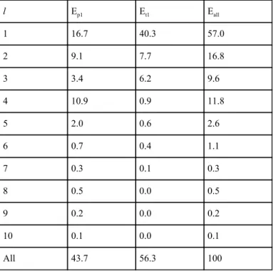
Table 4a. Relative energies for different spherical harmonic components of the magnetic map derived for April 2014. E ​p is the toroidal energy and E ​t is the toroidal energy whereas E​all is the sum of poloidal and toroidal energy, in percent. l E_​p1 E_​t1 E_​all 1 16.7 40.3 57.0 2 9.1 7.7 16.8 3 3.4 6.2 9.6 4 10.9 0.9 11.8 5 2.0 0.6 2.6 6 0.7 0.4 1.1 7 0.3 0.1 0.3 8 0.5 0.0 0.5 9 0.2 0.0 0.2 10 0.1 0.0 0.1 All 43.7 56.3 100

Table 4b. Same as Table 4a but for January 2015. l E​p2 E​t2 E​all 1 9.1 41.0 50.2 2 18.9 3.9 22.7 3 3.8 13.7 17.5 4 1.3 3.3 4.6 5 1.0 0.6 1.7 6 1.8 0.6 2.4 7 0.4 0.1 0.5 8 0.2 0.0 0.2 9 0.1 0.0 0.1 10 0.1 0.0 0.1 All 36.7 63.3 100

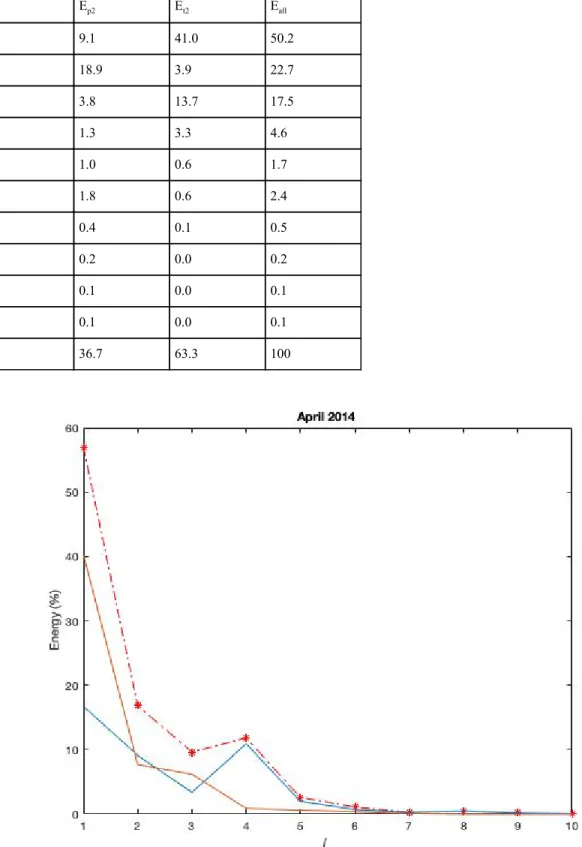
Figure 11. Plot of poloidal energy in blue, toroidal energy in orange, and total magnetic energy in red as a function of spherical harmonic angular degree ​l​ for the April 2014 magnetic map.

Figure 12. Same as Fig. 11 for the January 2015 magnetic map.

As an additional characteristic of the field, one can consider average strengths of different field vector components.The mean absolute strengths the radial, azimuthal and meridional field components have been listed in table (5). From the table it can be noted that the mean field is higher for the radial and meridional components in 2014 than in 2015, but the azimuthal field is almost the same. The total mean field is somewhat higher for the dataset taken in 2014, but the difference is only 3.8 G (13% of the total mean field).

Table 5. The average strength of the radial field, meridional field, azimuthal field and the total field for the magnetic field maps derived from April 2014 and January 2015 datasets. The mean field modulus is defined as

. <

B =

√

Field [G] April 2014 January 2015 mean |B_​r​| 12.9 8.8

mean |B​m​| 13.2 8.4

mean |B_​a​| 20.9 21.8

5. Summary and discussion

This study has presented analysis of the surface magnetic field of the young solar analogue

star π _​1 _{UMa. This work contributes to understanding evolution of the Sun’s magnetic field by}

looking at a star that represents a proxy of the Sun when it was just a few hundred million

years old. We started the analysis by downloading spectropolarimetric observations collected

in 2014 and 2015 from a public database. We then applied the LSD technique to derive

spectra of the mean Stokes _{​I and ​V line profiles. We assessed detection of the circular}

polarisation signatures and measured the mean longitudinal magnetic field from these

profiles. Then, these LSD Stokes profiles were modelled with the ZDI method to reconstruct

maps of stellar magnetic field topology and provide detailed information about the stellar

magnetic field.

The topology of the surface magnetic field of π _​1 _{UMa seems to be dominated by the}

azimuthal field component. Since we worked with only two sets of observations taken within

7 months of each other, it is hard to make far-reaching conclusions about long-term

variability of the stellar field. However, comparing to the earlier study in [7] of the same star,

the results of the magnetic field topology seem to agree. Also, the mean magnetic field

strengths were calculated from similar ZDI modelling of the observations obtained in 2007 in

their study. The field components strength values obtained in [7] were _​B​r=9 G, B _​m​=4 G _​and

B_​a​=21 G. These results agree very well with the mean magnetic field strengths derived in our

study based on observations from 2014 and 2015. Thus, it can be concluded that π _​1 _UMa

maintained approximately the same level of magnetic activity at these two epochs 7 years

apart.

Looking at figure (4) from reference [7] the distribution of E _​all is plotted as a function of L for

π_​1 _{UMa. Their result doesn’t differ much from ours (see figure (11,12)), because almost all of}

the total magnetic field energy is found in _{​l​=1-3 in both studies. In addition, the energy}

decreases as _{​l increases from 1 to 3 in both plots. The dipole component ​l​=1 contains most of}

the field energy. The results of the both ZDI studies show a dominantly toroidal field. This

agrees with the trend found in study [12] that younger/faster rotating stars tend to show

dominance of the toroidal component, while stars with increasing age or slower rotation rate,

like the Sun, tend to have a dominant poloidal component.

The difference in the mean characteristics of the global field of π _​1​_{UMa between April 2014}

and January 2015 is not so significant. The radial and meridional fields are somewhat weaker

in the later epoch and the azimuthal field is a little stronger. Perhaps we are observing

long-term activity cycle of this star with magnetic energy exchanging between the toroidal

(mainly azimuthal) and poloidal (mainly radial and meridional) components. In the radial

component the field is predominantly negative at the visible rotational pole for both epochs,

the azimuthal field components remains dominantly positive for both epochs. Perhaps, it is

not surprising that the change of the magnetic topology between the two epochs is not

significant because the two datasets were taken merely 7 months apart. Our analysis thus

suggests that the main properties of the global field topology of π _​1_{UMa remain stable on this}

time scale.

In reference [7] the magnetic field of π1 UMa was obtained with ZDI using observations

from 2007. The radial field was found to be negative at the north pole but has positive regions

around the equator and low latitudes close to the south pole. The meridional field is negative

in most areas, especially at the north pole. The azimuthal field is positive over the whole star,

and has the strongest spots at the stellar equator. This is very similar to the results obtained in

this project. There is no evidence that polarity switching has occurred because there is no

clear, systematic change in the sign of any of the magnetic field components in the three

epochs. However, since there is a big gap between the observational data from 2007 and

2014, several polarity reversals could have been missed between these years. The 2014 and

2015 data are 7 months apart and show the same field polarity, suggesting that, the magnetic

cycle might be one year or more. If no polarity switch has really occurred between 2007 and

2014 the magnetic cycle for the star might be 8 years or more. Moreover, the azimuthal

component is the strongest for all three epochs (2007, 2014 and 2015) and corresponds to a

larger mean field strength than radial and meridional field. This indicates persistent dominance of the horizontal fields likely associated with toroidal global field component.

Finally, this study has thereby presented analysis of the surface magnetic field of the young

solar analogue star π _​1 _{UMa. This work contributes to understanding evolution of the Sun’s}

magnetic field (which today have a much weaker global magnetic field of ~1 G) by looking

at a star that represents a proxy of the Sun when it was just a few hundred million years old.

6.References

[1] Petit, P., Dintrans, B., Solanki, S. K., et al. Magnetic geometries of Sun-like stars : impact

of rotation, _{​Proceedings of the Annual meeting of the French Society of Astronomy and}

Astrophysics Eds.: C. Charbonnel, F. Combes and R. Samadi_{​, 388, 80, 2008}

[2] H.Lammer et al. Variability of solar/stellar activity and magnetic field and its influence on

planetary atmosphere evolution. Earth Planets Space, 64, 179–199, 2012

[3] Kochukhov, O. Stellar Magnetic Fields. In J. Sánchez Almeida & M. Martínez González

(Eds.), Cosmic Magnetic Fields. (Canary Islands Winter School of Astrophysics, pp. 47-86).

Cambridge: Cambridge University Press. 2018

[4] Petit, P.; Louge, T.; Théado, S.; _{​Paletou, F.​; ​Manset, N.​; ​Morin, J.​; ​Marsden, S. C.​;}

Observations, Publications of the Astronomical Society of the Pacific, Volume 126, Issue 939, pp. 469, 2014

[5] J.-F. Donati and J. D. Landstreet. Magnetic Fields of Nondegenerate Stars. Annual Review of Astronomy & Astrophysics, 47:333–370, 2009.

[6] Claret,A. _{​A new non-linear limb-darkening law for LTE stellar atmosphere}

models. Calculations for -5.0 <= log[M/H] <= +1, 2000 K <= T _​eff <= 50000 K at several

surface gravities. A&A, 363, 1081-1190, 2000

[7] L. Rosén, O. Kochukhov, T. Hackman, and J. Lehtinen. Magnetic fields of young solar

twins. A&A 593, A35, 2016

[8] O. Kochukhov, T. Lüftinger, C. Neiner, E. Alecian, and the MiMeS collaboration.

Magnetic field topology of the unique chemically peculiar star CU Virginis. A&A _{​565, A83,}

2014.

[9] J.-F. Donati, M. Semel, B. D. Carter, D. E. Rees, and A. Collier Cameron. Spectropolarimetric observations of active stars. Mon. Not. R. Astron. Soc, 291, 658, 1997.

[10] Wade, G. A,. Donati, J-F,. Landstreet, J.D,. & Shorlin, S. L. S. High-precision magnetic

field measurements of Ap and Bp stars. Mon. Not. R. Astron. Soc,. 313, 823, 2000

[11] Kochukhov, O. & Wade, G. A, Magnetic Doppler imaging of α2 Canum Venaticorum in

all four Stokes parameters. Unveiling the hidden complexity of stellar magnetic fields, A&A, 513, A13, 2010

[12] Petit, P.; Dintrans, B.; Solanki, S. K.; Donati, J.-F.; Aurière, M.; Lignières, F.; Morin, J.;

Paletou, F.; Ramirez Velez, J,; Catala, C.; Fares, R. Toroidal versus poloidal magnetic fields

in Sun-like stars: a rotation threshold. Mon. Not. R. Astron. Soc _{​,. Volume 388, Issue 1, pp.}

80-88, 2008

[13] VALD3 (2018). Vienna Atomic Line Database [database] Retrieved from:

http://vald.astro.uu.se

[14] _{​Donati, J. -F.​; ​Semel, M.​; ​Carter, B. D.​; ​Rees, D. E.​; ​Collier Cameron, A.}

Spectropolarimetric observations of active stars. Mon. Not. R. Astron. Soc,. Volume 291,

Issue 4, p_{​p. 658-682, 1997}

[15] P. Janardhan.; K. Fujiki.; M. Ingale.; Susanta Kumar Bisoi.; and Diptiranjan Rout. Solar