Effect of house prices on regional migration : A cross-sectional analysis on Swedish municipalities

(1)

Effect of house prices on regional

migration

(2)

Acknowledgements

We, Dennis Johansson and Jonathan Molander, would like to take the opportunity to acknowledge a word of gratitude to the persons who have contributed with feedback and constructive criticism in our process of writing this thesis.

A big thank you to our mentor, Lina Bjerke, who has provided support and words of advice throughout this thesis.

Finally, we would like to give a special thanks to our friends and families, who have supported us during the time of this thesis.

Dennis Johansson Jonathan Molander

Jönköping International Business School May, 2019

(3)

Bachelor Thesis in Economics

Title: Effect of house prices on regional migration Authors: Dennis Johansson and Jonathan Molander Tutor: Lina Bjerke

Date: 2019-05-20

Key terms: Regional Economics, Labor mobility, Regional migration, House prices, Sweden

Abstract

The purpose of this thesis is to investigate what relation house prices have with regional migration in Sweden, with the interest of the study being to investigate how regional migration is affected by differentials in house prices and to see how it has affected migration choices for labor, and, to see if this relationship differed in 2007 and 2017. Theories surrounding regional house prices, regional migration, regional labor mobility, commuting, and accessibility are used to lay the foundation and support the empirical method. The regressions are run using cross-sectional data for the years 2007 and 2017. Whilst the literature review suggests that average house prices should have a negative relation towards in-migration, the conducted regression showcases a positive relation towards in-migration. Furthermore, the study concludes that there are many different variables that can affect regional migration. The results show that the effect of house prices has become weaker in the year 2017 compared to 2007, which could showcase that individuals have changed how they approach migration decision.

(4)

1 Introduction

The housing situation in Sweden has for a long time been an important matter for individuals that are looking for housing. There are many municipalities reporting that there is a shortage of housing (Hyresgästföreningen. 2019) and because of it, there is an excess demand. According to Boverket (2019), out of the 290 municipalities in Sweden, 240 municipalities assess a shortage in housing. Excess demand for housing with a shortage in supply leads to a continuous increase in prices, which is happening all around Sweden’s 290 municipalities. Between the years 2007 and 2017, the average price has gone up with 63 percent for houses (SCB, 2019). The total increase differs between the municipalities, with the bigger municipalities, close to metropolitan areas, showcasing a higher increase compared to the smaller municipalities that are located further away. The county of Stockholm and its municipalities have during the same period seen a general average increase of 71 percent, which is higher than the Swedish average. Comparing that with a smaller county such as Kalmar, the municipalities at the same time period showcasing a general average increase of only 44 percent, 19 percentage points lower than the Swedish average (SCB, 2019).

Individuals have for several generations migrated in seeking for new opportunities, with both urbanization causing individuals to migrate from rural to urban areas, and agglomeration causing larger centralized areas in the economy to grow even larger. This creates an incentive for in-migration, one of the reasons being an increase of employment opportunities. Stockholm’s county, for example, being the area with the highest population density, and the largest labor market in Sweden, creates incentives for people wanting to in-migrate and taking part of the opportunities in that area. Then with many people wanting to migrate into areas with limited housing, causing prices for housing to go up, will then force people to consider other alternatives when in-migration into the favored municipality is not possible. Alternatives being moving to a neighboring municipality, where the price for housing is lower, and the possibilities of commuting and general accessibility are high. Regional mobility possibilities allow people to work and live in different municipalities, which creates more opportunities that would otherwise not be possible. Good accessibility in municipalities, allow people to compete with other labor markets, and at the same time not be limited with the location of housing.

(6)

2 According to Eliasson, Lindgren and Westerlund. (2003), regional mobility is important as it contributes to efficient labor markets, increases in relative earnings and better job matching. Migration in the framework of this thesis will be defined as the move from one residence for an individual to another between different municipalities in Sweden. This type of migration can be just the change of one’s residence or it can be in connection with the change of one’s workplace. The theory states that an individual's mobility options are either to choose to migrate or to commute when changing workplace, as one will choose the alternative that maximizes their utility. Migrants specifically in this thesis will follow the assumptions of Sjaastad (1962) that individuals will choose to migrate into areas where they can achieve their highest total net benefit.

The purpose of this thesis is to investigate what relation house prices have had on regional migration in Sweden, with the interest of the study being to investigate how regional migration is affected by differentials in house prices and to see how it has affected migration choices for labor. The analysis uses cross-sectional data for all 290 municipalities in Sweden, with one regression being done for the year 2007 and one being done for 2017, with the intention to see if there is a difference in the relationship of the two variables for the different years.

(7)

3

2 Literature review

In this part of the thesis, previous literature will be covered to provide a theoretical background for house prices, migration, labor mobility, commuting and accessibility. Literature has been chosen with theories that is relevant to the research being conducted.

2.1 Regional house prices

According to Muellbauer & Murphy (1994), regional house prices can be determined by earnings within a region and in contiguous regions, the rate of return in regions and in contiguous regions that are lagged, and the regional population relative to the regional stock of housing. Findings by Bover, Muellbauer and Murphy. (1989) suggest that house prices in regions can rise due to a positive demand shock for labor. Since when labor demand goes up, then that can cause increases in relative earnings for labor, which in turn can cause the house prices to rise. Cameron & Muellbauers (1998) findings suggested that high relative house prices in regions and negative returns in the housing market can discourage in-migration.

Cannari, Nucci and Sestito (2000) found that housing prices can constrain migration between regions, this is because it will be harder for individuals to move with high regional differences in house prices. This can then in turn widen the gap for real earnings and employment rates between regions since labor markets can become inefficient, the findings suggest that the housing market is a large determinant in migration decisions.

2.2 Regional migration

Regional migration is when an individual or household moves within a region in a country, or from one region in a country to another region within the same country. There is a wide range of different factors that drive individuals to migrate, such as where an individual is in his/her lifecycle, as preferences for individuals change over their lifetime, and location characteristics can be important which vary between individuals (Lee, 1966). According to Greenwood (1985), there are differential characteristics of sending and receiving regions that provide a potential incentive for moving, and individual traits help condition the response to real utility differentials that may arise from these different characteristics. Work opportunities and general labor conditions are important, and something that may be

(8)

4 important is if there is a prevailing condition for housing markets (Molloy, Smith and Wozniak. 2011).

The human capital theory of migration presented by Sjaastad (1962) suggests that migration is seen as an investment in which an individual maximizes their own utility. According to the human capital theory, there can be many different components of the utility function for individuals which can be both monetary and non-monetary. Individuals cannot control all the components that affect their utility, but one does take that into account in their decision making when choosing where to live, to achieve their highest total net benefit. Sjastaad’s (1962) findings suggest that individuals are different and therefore have different preferences and so, the net-benefit for individuals will be different in specific locations. This can vary over the costs of living where house prices are a large cost, labor market experience, relative earnings and one's connection to the region. Therefore, migration choices for individuals will differ. In later research by Mincer (1978) the migration decisions were extended from the choice of one individual to the decision either being made as two individuals or a family. The findings suggest that the costs of migration can differentiate a lot for individuals within a household which can be connected to the regional labor market, earnings and connection to the region of origin.

In research by Bover, Muellbauer and Phimister (1989), it was found that higher house prices at a location lower the chances of migration into that region and higher relative earnings increase the chances of migration into regions. Eliasson et al. (2003) findings suggest that individuals consider relative earnings to be more important than nominal earnings. Since the increased earnings must offset the costs of migration and living costs in the new region with the price of housing being a large cost. Also, according to Eliasson et al. (2003) there are some major determinants for how an individual will pick a location when they migrate. Such as increased labor market opportunities, which will have a positive effect towards in-migration to a region, and how the market for housing is, since cheaper housing will have a positive effect on in-migration and overpriced housing will have a negative effect towards in-migration.

Pissarides & Wadsworth (1989) found that regions with an above average level of unemployment had more out-migrants than regions experiencing average or below average levels of unemployment. With outflows of migrants being greater from regions that

(9)

5 experience higher unemployment, that have low vacancies, and that have lower wages compared to other regions. In research by Cameron & Muellbauer (1998), it was found that migrants, which in this case are laborers, respond strongly towards unemployment in the case of differentials in relative earnings and in employment opportunities. According to Topel (1986), laborers will migrate from areas with high unemployment into more attractive regions with lower unemployment, because of more employment opportunities and so higher relative earnings. The findings of Pissarides & Wadsworth (1989) and McCormick (1997) supports this, as it was found that individuals living in regions with higher rates of unemployment have a larger propensity to move, rather than individuals living in regions with lower rates of unemployment.

2.3 Regional labor mobility

Eliasson et al. (2003) findings show that the structures of labor markets have a large influence on geographical labor mobility and the choice of mobility for individuals. There is a significant decrease in the chances to migrate from a region if labor has access to employment opportunities in one’s region of residence, and there is an increase in the chances of choosing to commute when there is access to employment opportunities outside one’s region of residence. The findings by Eliasson et al. (2003) also suggest that this can be seen through a harsh housing market, which decreases the chances of migration into contiguous regions.

According to Eliasson et al. (2003), There are different forms of mobility in labor, one being migration and the other one being commuting. Commuting and migration can influence the population in different regions, and regional commuting has become a large share of mobility in labor and is still increasing. Migration and commuting can affect how an individual will pick their home location and workplace in such a manner that they maximize their own utility by choosing the optimal travel time between their home and work. According to Battu et al. (2008), mobility and distance are important factors for individuals. The findings suggest that being a homeowner is a limitation when being employed, since homeowners are less likely to become employed in a more distant labor market which shows that being a homeowner does have a negative effect on labor mobility.

(10)

6 According to Dohmen (2005), laborers will search less actively for jobs at other locations if they become unemployed when moving costs are high, because with higher moving costs the losses from being unemployed will be relatively lower. Job searching is a function of mobility, in which lower mobility will lead to a decrease in the effectiveness of leading unemployed labor into open vacancies. The findings from Dohmen (2005) suggests that an individual’s own mobility depends upon the differences in earnings lost during the time of being unemployed and the cost of moving. Since if there is a rise in the benefits of being unemployed, or if there is a reduction in relative earnings, it will in turn reduce mobility and cause a rise in unemployment.

2.4 Commuting

In research by Cameron & Muellbauer (1998), it was found that relative labor market factors were even stronger for commuting than in the case of migration. There are different decisions towards migration into contiguous regions rather than more distant regions which can be implied by a tradeoff between commuting and migration. Since the fixed costs for migration is high and the costs of commuting do increase with time and distance. The tradeoff between commuting and migration can show that the housing market has had a significant effect on commuting, which acts in the opposite direction than that of migration. This is also supported by the findings of Johansson et al. (2003) where it is suggested that there is a difference between how individuals choose to commute with time differences. It was found that individuals’ response to time distances is non-linear which is because individuals are heterogeneous and have different preferences. Cameron & Muellbauers (1998) findings supported the findings of Jackman & Savouri (1992) that labor market variables should have weaker effects for contiguous regions, and housing market variables should have stronger effects for contiguous regions migration decisions. It means that when commuting is relatively cheap, individuals can decide where to live more independently of the decision where to work, in which the location decision acts stronger. These findings imply that for contiguous regions commuting can act as a help to offset the pressure that the housing market can put on regional labor markets.

Jackman & Savouri (1992) found that there is a flow of short distance movers, which are individuals who do change their place of residence between contiguous regions but do not change their workplace and it was also found that there are individuals who acquire jobs in regions that are different from their place of residence. Individuals who only change

(11)

7 their place of residence can take advantage of regional house prices when considering where to move and individuals that only change their workplace can take advantage of labor market opportunities in contiguous regions when deciding where to work by

commuting.According to Hoover & Renkow (2000), when individuals can choose their

place of living in connection with choosing their workplace, it creates many possible outcomes in the reallocation process which in turn then can be related to both patterns in migration and patterns in commuting. The findings from Hoover & Renkow (2000) suggest that individuals choose their place of living after preference, since individuals can choose to commute.

Cameron & Muellbauer (1998) suggested that commuting can offset inefficiency in regional labor markets when the costs of migration are higher than the gains from migration, with both earnings and employment opportunities having a positive effect towards both migration and commuting.

2.5 Accessibility

In Johansson et al. (2002) study on the effect of time distances on municipalities and both local and regional labor markets. They found that declining time distances increases the sizes of geographical labor markets, with the expansion of labor markets being determined by location decisions from both firms and households. Decisions made by firms and households are influenced by the attractiveness of a location which was measured as accessibility, the main idea is that accessibility does dictate both choices of migration and commuting. The findings suggest that a locations labor supply is related to the accessibility of jobs and the location of jobs can be explained by the accessibility to labor supply. This means that individuals locate themselves in regions where they have good accessibility to jobs, and firms locate themselves in regions where there is good accessibility to labor supply. In-commuting to a specific municipality can be related to the accessibility of jobs within the municipality and to the accessibility of labor supply in adjacent municipalities. Also, out-commuting from a municipality can be related to labor supply in a municipality and to the accessibility of jobs in adjacent municipalities.

(12)

8

3 Methodology

In this section, the hypothesis, the variables used in the empirical model, the data utilized with a descriptive analysis, and the empirical model are presented. Furthermore, each variable added to the model is discussed, along with its expected effect on the dependent variable shown in table 1. Finally, the method of this study, motivating the choice of econometric model is present.

3.1 Hypothesis

According to both previous research and theory, house prices should influence regional migration. The hypothesis in this thesis is that house prices should have a significant effect on regional migration, and to see if the relationship between house prices and regional migration has changed between 2007 and 2017.

3.2 Variables

Migration ratio (MR)

The dependent variable for this thesis is migration ratio which is measured as a ratio on a municipal level. The ratio is estimated as the in-migration divided by out-migration in absolute values. With in-migration being the number of individuals migrating into a municipality and out-migration being the number of individuals migrating from a municipality.

Example for clarification reason: an MR value of 1,17 (e.g. 117 people move into a municipality, divided by 100 people moving out from the municipality) indicates that there are more people migrating into that municipality. An MR value of 0,89 (e.g. 89 people moving into a municipality divided by 100 people moving out from the municipality) indicates that there are more people migrating from that municipality.

Average house price (AHP)

The independent variable average house price in this thesis refers to the average house prices on a municipal level. The variable will be estimated in its absolute value in thousands of Swedish crowns.

(13)

9

Average full-time earnings (AFTE)

The independent variable average full-time earnings are the total average full-time earnings from all the individuals living in the municipality. The variable will be estimated in its absolute value in thousands of Swedish crowns.

Commuting (COM)

The independent variable commuting is a ratio between the day and night population in municipalities and refers to the number of people who commute to other municipalities for work. Individuals will look over their migration choices when choosing where to work and to live, with commuting being an alternative to migrating.

Example for clarification reason: a COM value of 1,20 (e.g. 12000 individuals that work in a municipality but do not live there, divided by 10000 individuals living and working municipality) indicates that there are more individuals commuting into a municipality for work than individuals who work and live there. A COM value of 0,8 (e.g. 8000 individuals that work in a municipality but do not live there, divided by 10000 individuals living and working municipality) indicates that there are fewer individuals that commute into the municipality than individuals that work and live in the municipality.

Unemployment rate (UP)

The independent variable unemployment refers to the percentage of unemployed individuals in the labor force on a municipal level.

Accessibility (A)

The independent variable accessibility is the total accessibility for individuals living and working in a specific municipality. The variable will be derived from the individual’s being active in the labor force at a municipal level to see what their accessibility is in their corresponding region. A higher value for accessibility means that there are more opportunities for individuals living in a municipality and a lower value means that there are less opportunities for individuals living in a municipality.

(14)

10

Population density (POPD)

The independent variable population density refers to the population density on a municipal level. It shows how concentrated or sparse each municipality is in Sweden, and it is measured as the inhabitants per square kilometer.

Dummy variable (D)

A dummy variable will be used for the cities Stockholm, Göteborg and Malmö. Since larger cities tend to be different from smaller municipalities in many ways which comes with having a large labor market, large population and much higher cost of living.

Table 1. Abbreviations, definitions, and expected effect of variables

Abbreviations Definitions Expected Effect

MR Migration Ratio in municipality m

AHP Average House Prices in municipality m

-AFTE Average Full-time Earnings in municipality m +

COM Commuting Ratio in municipality m

-UP Unemployment in municipality m

-A Accessibility in municipality m +

POPD Population Density in municipality m +

D Dummy variable

-3.3 Data

The collected data in this thesis will be cross-sectional which will be sampled from two different points in time. The first year will be 2007, which is used as it was before the financial crisis and the economy was stable. The second year will be 2017 which is after the great recession and has allowed the economy to stabilize, there have been policy changes in the mortgage market (Finansinspektionen, 2019) between both time points which have had an impact on the housing market. The data was collected for all the 290 municipalities in Sweden, so there will be 290 observations for each year. All the data collected is from SCB (Statistics Sweden) and RAPS (Tillväxtverket).

To get an overview of what the data set looks like, the descriptive statistics for both the dependent variable (MR) and variable of interest (AHP) will be discussed. The data for all the municipalities is included in Tables 2 & 3 down below. In case of any extreme or

(15)

11 otherwise noteworthy values for the other variables, then that will also be mentioned. This section will finish with a correlation analysis.

Table 2. Descriptive Statistics for the year 2007

Descriptive Statistics for the year – 2007

Mean Median Std. dev Max Min

MR 0,954 0,964 0,173 1,608 0,394 AHP 1317 957 1001 6528 226 UP 0,050 0,489 0,017 0,114 0,015 AFTE 212,6 206,2 27,2 417,2 179,2 COM 0,884 0,903 0,196 2,061 0,364 A 59629 33316 74722 436759 1902 POPD 130,722 26,250 441,293 4228,200 0,200

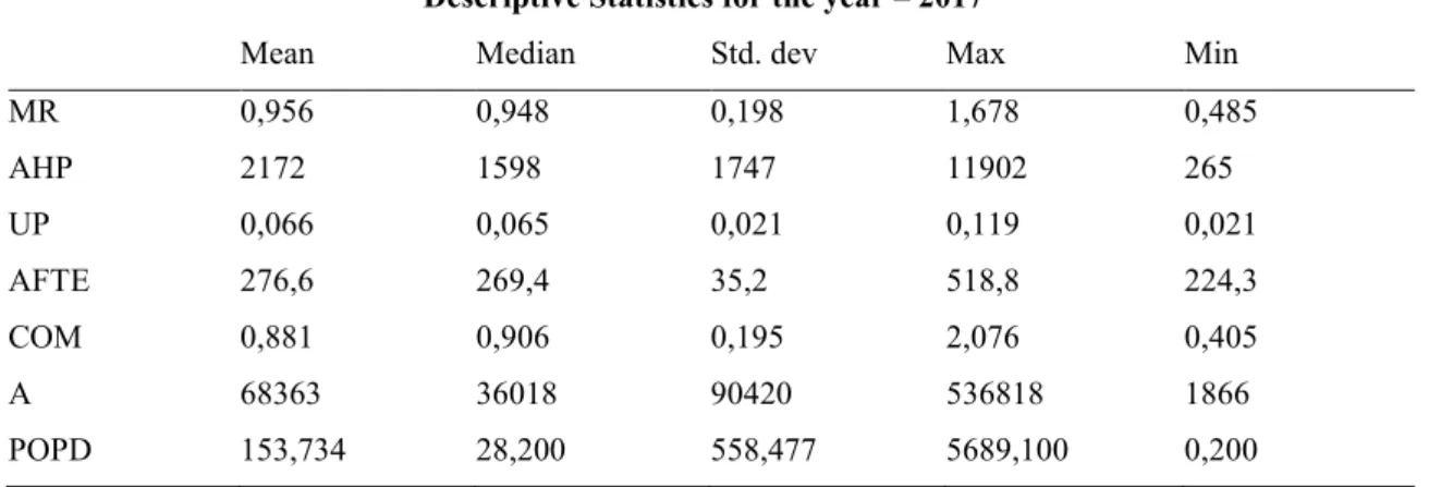
Table 3. Descriptive Statistics for the year 2017

Descriptive Statistics for the year – 2017

Mean Median Std. dev Max Min

MR 0,956 0,948 0,198 1,678 0,485 AHP 2172 1598 1747 11902 265 UP 0,066 0,065 0,021 0,119 0,021 AFTE 276,6 269,4 35,2 518,8 224,3 COM 0,881 0,906 0,195 2,076 0,405 A 68363 36018 90420 536818 1866 POPD 153,734 28,200 558,477 5689,100 0,200

The mean for the dependent variable migration ratio (MR) had a value of 0,954 in 2007 and a value of 0,956 in 2017. That means that the average value for the migration ratio is below one across all municipalities in Sweden, which could suggest that more people are migration out from municipalities rather than migrating in. The value for the mean had increased from 2007 to 2017 which means that the value has gone up over time. The maximum value for the variable was 1,608 in 2007 and 1,678 in 2007, the minimum

(16)

12 value in 2007 was 0,394 and 0,485 in 2017. Since the maximum and minimum values for both the years 2007 and 2017 differ a lot then that means that there are municipalities with far higher in-migration and as well municipalities with far higher out-migration.

The mean for the independent variable average house prices (AHP) had a value of 1317 in 2007 and a value of 2172 in 2017. It is interesting that there has been such a large increase in the value of from 2007 to 2017. Since this would suggest that the average house prices in Sweden has seen a significant increase between the years 2007 and 2017. The maximum value for the variable being 6528 in 2007 and 11902 in 2017, the

minimum value in 2007 was 226 and 265 in 2017. This explains that there are large differences in the variable average house prices across Sweden and that the difference has become even greater in the year 2017.

The independent variable accessibility (A) will be discussed a bit more as the values for the variable do differ a lot both with the minimum and maximum values. As the

maximum value was 436759 in 2007 and 536818 in 20017 and the minimum value was 1902 in 2007 and 1866 in 2017. This could suggest that larger municipalities have started to become even more centralized since the maximum value had gone up for 2017 and the minimum value had gone down in 2017. It does also show that there is a widespread for how good accessibility there is across the municipalities in Sweden. The standard deviation is also very large for both the years, with a value of 74722 in 2007 and a value of 90420 in 2017. Having a high standard deviation can cause problems in the model, which will be discussed later.

The correlations between the dependent and independent variables for 2007 and 2017, with their significances according to the Pearson method are presented in table 4 down below. Like the previous section, descriptive statistics, all municipalities are included.

(17)

13

Table 4. Correlation between dependent and independent variables.

Migration Ratio (MR) Pearson Correlation

Correlation 2007 Correlation 2017 AHP 0.598* 0.488* AFTE 0.459* 0.483* COM -0.267* -0.330* UP -0.383* -0.551* A 0.397* 0.369* POPD 0.237* 0.112** *Significant at 1% level **Significant at 10% level N = 290 DF = 290 – 2 = 288

In table 4, the correlation between the dependent variable MR, and independent variables are illustrated. The results show that the variable of interest, AHP, is significant at the 1 percent level in both 2007 and 2017. The other independent variables, AFTE, COM, UP and A, is just as the variable of interest, significant at the 1 percentage level for both 2007 and 2017. The independent variable, POPD, is significant at the 1 percent level in 2007, but is only significant at the 10 percent level in 2017.

The overall results showcase that the independent variables are significant with the dependent variable MR, and that there has not been any difference in the independent variables after 2007, since all 6 variables were significant in both years, with the exception of POPD, which were significant at the 10 percent level but not at the 1 percent level. The correlation between the dependent variable and independent variables have had different changes between 2007 and 2017. The independent variables; AHP, A and POPD have had an overall decrease in correlation with the dependent variable, and the independent variables; AFTE, COM and UP showcased an increased correlation. The variables that had the highest correlation in both observed years were UP (-0.383, -0.551), AHP (0.598, 0.488) and AFTE (0.459, 0.483), with respective numbers representing 2007 and 2017. UP being negatively correlated with the dependent variable, and both AHP, as well as AFTE, being the highest positively correlated variables.

(18)

14

3.4 Regression Model

To be able to answer the hypothesis, the following regression model has been estimated and is used to obtain a view on regional migration:

MRm = αm + Log(AHPm) + Log(AFTEm) + COMm + Log(UPm) + Log(Am) + Log(POPDm) + Dm + m

This linear multiple regression model, through the OLS, is run with the data for the years 2007 and 2017. There are two sets of data for all municipalities that are being individually measured. In the model, the m subscript represents each municipality. The variable AHP is the variable of interest, and UP, COM, AFTE, A, POPD and the dummy variable D being included as control variables.

The independent variables; AHP, AFTE, UP, A and POPD, will all be in logged form. The reason being the values in each variable tend to differ a lot and might cause heteroscedasticity problems i.e. the standard errors are non-constant, also it made more sense for the model to have them in their logged form which was seen through a Ramsey RESET test to see that the model was not miss specified (See appendix 1.4). The regression model was tested for multicollinearity by looking at the variance inflation factors (see appendix 1.3), to see that the independent variables aren’t heavily correlated in the model, which will be discussed in the empirical results. A test for normality was also done to see that the results were consistent and not biased. The model was as well tested for heteroscedasticity to see that the standard errors were normally distributed (see appendix 1.2), the results will be discussed in the empirical results (Gujarati & Porter, 2009).

(19)

15

4 Empirical results

In this part of the thesis, the results from the regressions are showed and analyzed from the years 2007 and 2017. There are three different equations used for each year with the variable population density being excluded in the second equation as it can be seen through the variance inflation factors that multicollinearity is present. This is probably due to population density being correlated with accessibility and average house prices. In the third equation we have accessibility, population density and the dummy being excluded in the to get results without variables that differentiates smaller municipalities with the bigger municipalities. Tests for non-normality showed no significant problems that could either lead to bias or misleading results. However, some sort of heteroscedasticity seems to be present in the model, which might be due to how the data was gathered. As the values for the larger municipalities tend to come earlier in the samples which is mainly because of how the samples are gathered across Sweden and this could cause the standard errors to follow a linear pattern and become non-constant. That’s why the Huber-white method for consistent standard errors and covariance’s was used in the model. The results are shown in table 5 below.

(20)

16

Table 5. Regression Models

2007 Regression Model 2017 Regression Model

Variables Eq. (1) Eq. (2) Eq. (3) Eq. (1) Eq. (2) Eq. (3)

Constant 1.393 1.489 1.464 2.527 2.328 2.134 Log(AHP) 0.185* (0.0250) 0.179* (0.0214) 0.185* (0.0199) 0.132* (0.0267) 0.148* (0.0225) 0.186* (0.0194) Log(AFTE) -0.358* (0.1267) -0.362* (0.1233) -0.341* (0.1231) -0.603* (0.1643) -0.594* (0.1635) -0.519* (0.1691) COM -0.147* (0.0372) -0.151* (0.0364) -0.171* (0.0366) -0.163* (0.0475) -0.161* (0.0467) -0.206* (0.0448) Log(UP) -0.051 (0.0372) -0.052 (0.0368) -0.059) (0.0366) -0.229* (0.0400) -0.217* (0.0376) -0.194* (0.0372) Log(A) 0.017 (0.0117) 0.013 (0.0110) - - 0.028** (0.0140) 0.039* (0.0114) - - Log(POPD) -0.006 (0.0119) - - - - 0.0130 (0.0121) - - - - DUMMY -0.144* (0.0458) -0.150* (0.0434) - - -0.164* (0.0378) -0.154* (0.0379) - - R2 _0.457 _0.457 _0.448 _0.542 _0.540 _0.519

Standard errors in parenthesis

* = Significant at the 1% level ** = Significant at the 5% level

*** = Significant at the 10% level

All the results from the equations will be discussed even though multicollinearity was present in the first equation. The results from equation one in 2007 provide the following information. Average house prices which is the variable of interest is significant on the one percent level, the positive sign on the coefficient implies that there is a positive relationship between average house prices and migration ratio. This implies that when average house prices is higher, migration ratio will be higher. The variables average full-time earnings, commuting and dummy are all significant at the one percent level and the coefficients for average full-time earnings, commuting and dummy are negative which implies that an increase in their value can have a negative effect towards migration ratio. The value for

R2 is 0,457 which shows the goodness of fit for the model and in which the value can vary

(21)

17 The results from equation two in 2007 where population density is removed, showed that the variables that were significant in equation one is still significant, and the signs of the coefficients are still the same. The difference is that the value has changed for the coefficients average house prices, average full-time earnings, commuting and the dummy. The value of average house prices has decreased, which shows that the relationship with migration ratio har become weaker. The coefficients for average full time earnings, commuting and dummy have increased, which implies a stronger negative relationship

with migration ratio. The value of R2 has not changed, which implies that the independent

variables are as explanatory for the dependent variable as in equation one.

In equation three for 2007, where the variables; accessibility, population density, and dummy are excluded, the regression showcased a similar result as the previous two equations with all variables being significant. Unemployment rate is still insignificant, but both average house prices and commuting have increased their coefficients, which implies a stronger relationship with migration ratio. Average full-time earnings coefficient has decreased, indicating a weaker negative relationship than both equation one and equation two. R2 has decreased, but that can be explained by the decrease in the amount of

used independent variables in the regression.

Next up is the results from the 2017 equations were the outcomes will be discussed and the changes from 2007 to 2017 will be covered as well.

The results from equation one in 2017 provide the following information. The variable AHP is still significant at the one percent level. The value of the coefficient for average house prices has decreased compared to 2007 which implies that the relationship between average house prices and migration ratio has become weaker. The variables average full-time earnings, commuting and dummy that were significant in 2007 are still significant. The value of the coefficients for the variables average full-time earnings, commuting and dummy have increased from 2007, which implies that the relationship is now stronger between the variables and migration ratio. The variable unemployment rate has become significant at the one percent level, accessibility has become significant at the five percent level, unemployment rate showing a negative relationship with migration ratio, and accessibility showing a positive relationship. The value of R2has gone up which

(22)

18 In the equation two from 2017 where population density is removed, we can see that the variable accessibility is now significant at the one percent level, all the variables that were significant in equation one are still significant. The value of average house prices and accessibility has gone up, which implies a stronger relationship with MR. The independent variables; average full-time earnings, commuting, unemployment rate and dummy shows a decreased relationship with migration ratio, indicating a lesser negative relationship with

migration ratio. The value of R2has gone down in the second equation which suggests that

the first equation is better at explaining the dependent variable.

In the third and last equation for 2017 where the variables; accessibility, population density and dummy are excluded, the regression showcased a similar result as the previous two equations. All variables are significant and there were no changes in the respective signs. The coefficients of average house prices and commuting have both increased, with average house prices showing an increased positive relation with migration ratio, and commuting showing a stronger negative relationship with migration ratio. The variables unemployment rate and average full-time earnings both showing a decrease in the coefficients, both having a lesser negative relation with migration ratio than in the previous equation for 2017. R2 is smaller than equation 1 and equation 2, which can be explained by

(23)

19

5 Discussion

In this part of the thesis, there will be a discussion around the empirical results that were achieved through the regressions to see if the hypothesis does suffice with what was found for the years 2007 and 2017.

When looking at the variable of interest which is average house prices, there is a positive relationship with the migration ratio in both 2007 and 2017 with the variable being significant in all cases. It is interesting that the relationship is positive, since according to Cameron & Muellbauer (1998), higher house prices should discourage in-migration. The results indicate that as house prices increase, the migration ratio should do the same. This can be because as regions and regional labor markets grow larger, then that creates an incentive for in-migration but that does also in turn increase house prices. This follows the theory from Bover, Muellbauer et al. (1989) about positive demand shocks for labor. The result for the average house prices can then indicate that individuals consider better labor markets to be a more attractive location characteristic, and thus that can have a larger effect when picking where to live, rather than house prices in that location. This could be in accordance with urbanization that people move from rural to urban areas to get better labor market opportunities even though the price of housing will usually be higher, and with agglomeration that larger economic areas tend to become even more centralized and grow even larger.

The variable average full-time earnings was not fully consistent with theory and what was predicted. That is why the variable average full-time earnings will be discussed a bit more. According to Sjaastad (1962), Topel (1986), Bover, Muellbauer et al. (1989) and Cameron & Muellbauer (1998), higher earnings should be an attractive location characteristic in municipalities which should create an incentive for in-migration. The results show that higher earnings do have a negative effect on the migration ratio. But as theory then also predicts individuals that migrate do consider relative earnings to be more important than nominal (Eliasson, Lindgren et al. 2003), which is why the results can be negative as the increased earnings do not necessarily offset living costs. It is also notable to say that individuals can pick the alternative to commute instead of migrating as suggested by Jackman & Savouri (1992), Cameron & Muellbauer (1998) and Renkow & Hoover (2000) which could be why the resulting coefficient is negative. Furthermore, it is interesting that

(24)

20 both average house prices and average full-time earnings had a different sign on the coefficient than what was expected, as both variables can affect the other one. If house prices rise, then the earnings must go up by relatively the same to make in-migration beneficial (Eliasson, Lindgren et al. 2003). The same goes for earnings as an increase in demand for labor can raise earnings and then also, regional house prices (Bover, Muellbauer et al. 1989). The result could indicate that increases in earnings create an incentive for individuals to commute since as stated by Cameron & Muellbauer (1998) migrating takes time and has a large fixed cost. This might be why average house prices have a positive effect towards the migration ratio, since prices of housing could take time to adjust. Then when individuals migrate into a region, they might already have acquired higher earnings which then in turn raise house prices.

The variables commuting, unemployment rate and accessibility were consistent with theory and the results followed what was predicted. What is interesting is that the variables can have a considerable effect on how individuals choose to migrate and, that an increase in house prices can affect these variables both negatively and positively. The commuting variable showed a negative relationship with the migration ratio which can be connected to house prices and as suggested by Cameron & Muellbauer (1998) higher house prices in a region do discourage in-migration and therefore individuals can look for other alternatives and can choose to commute. The unemployment variable which was significant in 2017 showed a negative relationship with the migration ratio and as stated by Topel (1986), Pissarides & Wadsworth (1989) and McCormick (1997), high unemployment in a region does increase the chances of migrating to another region. This could work in accordance with house prices as regions with more attractive and larger labor markets with lower unemployment can have higher house prices, which can also be a reason why house prices do have a positive relationship with migration. The accessibility variable showed a positive relationship towards migration which followed the theory from Johansson, Klaesson et al. (2002). This can as well be a reason why house prices do have a positive relationship with migration because accessibility is an attractive location characteristic and it is possible that more attractive locations have higher house prices.

Then there is the other purpose of seeing if there was a difference in the relationship between the years 2007 and 2017 for the variables. From the regression results, shown in Table 5, one can see that the effect of average house prices on the migration ratio had a

(25)

21 smaller effect in 2017 compared to 2007. The effect is still on the positive side with a coefficient of 0.132 in equation one, 0.148 in equation two and 0.186 in equation three, it is moving closer towards our previous expectation of a negative effect towards the migration ratio for the first two equations, and equation three is almost on the exact same value as the equations in the year 2007. Both commuting and unemployment rate showcased an increase in the coefficients from 2007 to 2017 which shows that both variables had an increased negative effect towards migration ratio, with commuting still being highly significant and unemployment rate now being highly significant. This shows that there has been an increase in the number of people that choose to commute and that there has been a drastic change in how individuals react to differentials in the unemployment rate when considering migration.

This thesis can include some limitations. For starters, migrants are individuals who move to maximize their total net benefits, but individuals are heterogeneous and do not necessarily respond to changes in the same way or migrate for the same reasons. There is a wide range of factors that can determine migration and not everything can be included in the model. All individuals that are in the labor force do not necessarily own their place of residence.

(26)

22

6 Conclusion

After conducting the regressions and reviewing the results in this thesis, we cannot reject our hypothesis. House prices could have had a significant effect on regional migration and there has been a change in the relationship between the dependent variable migration ratio and the independent variable average house price between the years 2007 and 2017.

In conclusion, there are many different variables that can affect regional migration. It was found that an increase in the average house prices for municipalities tends to increase the migration ratio, the results are interesting since it means that there must be other

dynamics that also lie behind how individuals respond to differentials in house prices. The results show that the effect of house prices has become weaker in the year 2017 compared to 2007, which could showcase that laborers have changed how they approach migration decisions.

For future research one could try to find the dynamics that lie behind how individuals behave towards changes in house prices and what exactly the dynamics are that affect it. Especially one could investigate the relationship between house prices and relative earnings even more.

(27)

23

7 References

Battu, H., Ma, A. and Phimister, E. (2008). "Housing Tenure, Job Mobility and Unemployment in the UK." The Economic Journal 118(527): 311-328.

Bover, O., Muellbauer, J. And Murphy, A. (1989). "HOUSING, WAGES AND UK LABOUR MARKETS." Oxford Bulletin of Economics & Statistics 51(2): 97-136.

Boverket. Bostadsmarknadsenkäten. (2019). Retrieved May 05, 2019,

from https://www.boverket.se/sv/samhallsplanering/bostadsmarknad/bostadsmarknaden/

bostadsmarknadsenkaten/

Cameron, G. and J. Muellbauer (1998). "The Housing Market and Regional Commuting and Migration Choices." Scottish Journal of Political Economy 45(4): 420-446.

Cannari, L., Nucci, F. and Sestito, P. “Geographic labour mobility and the cost of housing: evidence from Italy.” Applied Economics 32(14): 1899-1906.

Dohmen, T. J. (2005). "Housing, mobility and unemployment." Regional Science and

Urban Economics 35(3): 305-325.

Eliasson, K., Lindgren, U. and Westerlund, O. (2003). "Geographical Labour Mobility: Migration or Commuting?" Regional Studies 37(8): 827-837.

Finansinspektionen. Amortization requirement for new mortgages. (2016). Retrieved

March 14, 2019, from

https://www.fi.se/en/published/press-releases/2016/amortisation-requirement-for-new-mortgages/#dela

Greenwood, M. J. (1985). Human Migration: Theory, Models, and Empirical Studies*. Journal of RegionalScience, 25(4): 521.

https://doi-org.proxy.library.ju.se/10.1111/j.1467-9787.1985.tb00321.x

Gujarati, D. N., & Porter, D. C. (2009). Basic econometrics (5th edition). Boston, Mass: McGraw-Hill.

(28)

24 Hoover, D. and Renkow, M. (2000). "Commuting, Migration, and Rural-Urban Population Dynamics." Journal of Regional Science 40(2): 261-287.

Jackman, R. and Savouri, S. (1992). "REGIONAL MIGRATION VERSUS REGIONAL COMMUTING: THE IDENTIFICATION OF HOUSING AND EMPLOYMENT FLOWS." Scottish Journal of Political Economy 39(3): 272-287.

Johansson, B., Klaesson, J. and Olsson, M. (2002). "Time distances and labor market integration." Papers in Regional Science 81(3): 305-327.

Johansson, B., Klaesson, J. and Olsson, M. (2003). "Commuters’ non-linear response to time distances." Journal of Geographical Systems 5(3): 315-329.

Lee, E. (1966). A Theory of Migration. Demography, 3(1): 47-57. Retrieved from http://www.jstor.org/stable/2060063

McCormick, B. (1997). "Regional unemployment and labour mobility in the UK." European Economic Review 41(3): 581-589.

Mincer, J. (1978). "Family Migration Decisions." Journal of Political Economy 86(5): 749-773.

Murphy, A. and J. Muellbauer (1994). “Explaining regional house prices in the UK,"

Working Papers 199421, School of Economics, University College Dublin.

Molloy, R., Smith, C., L. and Wozniak, A. (2011). "Internal Migration in the United States." Journal of Economic Perspectives 25(3): 173-196.

Pissarides, C. A. and Wadsworth, J. (1989). "Unemployment and the Inter-Regional Mobility of Labour." The Economic Journal 99(397): 739-755.

Sjaastad, L. A. (1962). "The Costs and Returns of Human Migration." Journal of Political

(29)

25 Statistics Sweden (2018). Medelpriser för småhus 2017 per kommun med prisförändringar under 1, 5, 10 och 20 år. Retrieved April 12, 2019, from https://www.scb.se/hitta- statistik/statistik-efter-amne/boende-byggande-och-bebyggelse/fastighetspriser-och-

lagfarter/fastighetspriser-och-lagfarter/pong/tabell-och- diagram/kommunstatistik/medelpriser-for-smahus-per-kommun-med-prisforandringar-under-1-5-10-och-20-ar/

Topel, R. H. (1986). "Local Labor Markets." Journal of Political Economy 94(3): S111-S143.

(30)

26

Appendix

1.1 Correlation Table Table 1.1.1:

Correlation Table - 2007

MR AHP AFTE COM UP A POPD

MR 1 0.598 0.459 -0.267 -0.383 0.397 0.237 AHP 0.598 1 0.778 -0.201 -0.435 0.736 0.618 AFTE 0.459 0.778 1 -0.261 -0.480 0.638 0.471 COM -0.267 -0.201 -0.261 1 0.246 -0.262 -0.100** UP -0.383 -0.435 -0.480 0.246 1 -0.328 -0.176 A 0.397 0.736 0.638 -0.262 -0.328 1 0.770 POPD 0.237 0.618 0.471 -0.100** -0.176 0.770 1 **=10% level Table 1.1.1: Correlation Table – 2017

MR AHP AFTE COM UP A POPD

MR 1 0.488 0.483 -0.330 -0.551 0.369 0.112** AHP 0.488 1 0.877 -0.060*** -0.510 0.810 0.623 AFTE 0.483 0.877 1 -0.190 -0.644 0.662 0.420 COM -0.330 -0.060*** -0.190 1 0.301 -0.044*** 0.207 UP -0.551 -0.510 -0.644 0.301 1 -0.334 -0.151* A 0.369281 0.810 0.662 -0.044*** -0.334 1 0.722 POPD 0.112** 0.623 0.420 0.207 -0.151* 0.722 1 *=5% level **=10% level

***=Not Significant at any given level

1.2 Heteroskedasticity Test Table 1.2.1

Heteroskedasticity Tests 2007 – equation 1: Heteroskedasticity Test: Breusch-Pagan-Godfrey

F-statistic 0.965933 Prob. F(7,282) 0.4564

Obs*R-squared 6.790529 Prob. Chi-Square(7) 0.4510

Scaled explained SS 10.13211 Prob. Chi-Square(7) 0.1812

(31)

27

Table 1.2.2

Heteroskedasticity Test: White

Heteroskedasticity Tests 2007 – equation 2:

Table 1.2.3

Heteroskedasticity Test: Breusch-Pagan-Godfrey

Table 1.2.4

Table 1.2.5

Table 1.2.6

Heteroskedasticity Tests 2017 – equation 1: Table 1.2.7

(32)

28

Table 1.2.8

Table 1.2.9

Table 1.2.10

Table 1.2.11

Table 1.2.12

(33)

29

1.3 Variance Inflation Factors Table 1.3.1

VIF 2007 – equation 1: Variance Inflation Factors

Sample: 1 290

Included observations: 290

Variable CoefficientVariance

Uncentered VIF Centered VIF C LOG(AHP) LOG(AFTE) COM LOG(UP) LOG(A) LOG(POPD) DUMMY 0.379926 0.000627 0.016060 0.001385 0.001382 0.000138 0.000142 0.002101 7327.689 608.4129 8911.318 25.01174 251.4110 304.5247 45.71723 1.684492 NA 5.743459 3.640414 1.332298 2.034806 2.901325 7.932734 1.616967 Table 1.3.2 VIF 2007 – equation 2: Variance Inflation Factors

Sample: 1 290

Uncentered VIF Centered VIF C LOG(AHP) LOG(AFTE) COM LOG(UP) LOG(A) DUMMY 0.285846 0.000458 0.015224 0.001330 0.001354 0.000122 0.001889 5514.306 444.3195 8446.374 24.03650 245.8442 270.0900 1.519809 NA 4.174890 3.332792 1.275614 1.992091 2.482244 1.458047 Table 1.3.3 VIF 2007 – equation 3: Variance Inflation Factors

Sample: 1 290

Variable CoefficientVariance UncenteredVIF CenteredVIF

C LOG(AHP) LOG(AFTE) COM LOG(UP) 0.290568 0.000395 0.015163 0.001342 0.001344 5230.161 353.5710 7840.476 21.68717 228.3421 NA 3.166187 3.214256 1.126387 1.894474

(34)

30

Table 1.3.4

VIF 2017 – equation 1: Variance Inflation Factors

Sample: 1 290

Uncentered VIF Centered VIF C LOG(AHP) LOG(AFTE) COM LOG(UP) LOG(A) LOG(POPD) DUMMY 0.627463 0.000714 0.027012 0.002257 0.001605 0.000197 0.000146 0.001434 11787.55 754.4393 15968.68 39.38089 220.5549 427.3409 48.34445 2.301788 NA 7.198478 4.857689 1.546211 2.759105 5.327960 10.32048 2.104313 Table 1.3.5 VIF 2017 – equation 2: Variance Inflation Factors

Sample: 1 290

Uncentered VIF Centered VIF C LOG(AHP) LOG(AFTE) COM LOG(UP) LOG(A) DUMMY 0.570731 0.000509 0.026737 0.002181 0.001415 0.000131 0.001439 10522.04 528.2630 15510.70 36.95955 191.5512 278.5098 1.905488 NA 4.948832 4.895956 1.454865 2.507552 3.317477 1.768558 Table 1.3.6 VIF 2017 – equation 3: Variance Inflation Factors

Sample: 1 290

Uncentered VIF Centered VIF C LOG(AHP) LOG(AFTE) COM LOG(UP) 0.619847 0.000380 0.028612 0.002010 0.001384 10403.26 352.1023 15072.69 29.40713 169.7886 NA 3.190293 4.841443 1.131859 2.434490

(35)

31

1.4 Ramsey Reset Test Table 1.4.1

Ramsey RESET test 2007: Ramsey RESET test

Specification: MR C LOG(AHP) LOG(AFTE) COM LOG(UP) LOG(A) LOG(POPD) DUMMY Value Df Probability t-statistic 1.732248 281 0.0843 F-statistic 3.000682 (1,281) 0.0843 Likelihood ratio 3.080371 1 0.0792 Table 1.4.2

Ramsey RESET test 2017: Ramsey RESET test

Specification: MR C LOG(AHP) LOG(AFTE) COM LOG(UP) LOG(A) LOG(POPD) DUMMY

Value Df Probability

t-statistic 1.589754 281 0.1130

F-statistic 2.527317 (1,281) 0.1130

Effect of house prices on regional migration : A cross-sectional analysis on Swedish municipalities