Time Series Forecasting using ARIMA Model: A Case Study of Mining Face Drilling Rig

(1)

Time Series Forecasting using ARIMA Model

A Case Study of Mining Face Drilling Rig

Hussan Al-Chalabi, Yamur K. Al-Douri and Jan Lundberg

Division of Operation and Maintenance Engineering Luleå University of Technology

Luleå, Sweden

E-mail: {hussan.hamodi, yamur.aldouri, jan.lundgerg}@ltu.se

Abstract— This study implements an Autoregressive Integrated Moving Average (ARIMA) model to forecast total cost of a face drilling rig used in the Swedish mining industry. The ARIMA model shows different forecasting abilities using different values of ARIMA parameters (p, d, q). However, better estimation for the ARIMA parameters is required for accurate forecasting. Artificial intelligence, such as multi objective genetic algorithm based on the ARIMA model, could provide other possibilities for estimating the parameters. Time series forecasting is widely used for production control, production planning, optimizing industrial processes and economic planning. Therefore, the forecasted total cost data of the face drilling rig can be used for life cycle cost analysis to estimate the optimal replacement time of this rig.

Keywords- ARIMA model; Data forecasting; Mining face drilling rig.

I. INTRODUCTION

Time series forecasting predicts future data points based on observed data over a period known as the lead-time. The purpose of forecasting data points is to provide a basis for production control and production planning and to optimize industrial processes and economic planning. The major objective is to obtain the best forecast, i.e., to ensure that the mean square of the deviation between the actual and the forecasted values is as small as possible for each lead-time [1]. Over the past few decades, much effort has been devoted to the development and improvement of time series forecasting models [2].

Traditional models for time series forecasting, such as the Box–Jenkins or the Autoregressive Integrated Moving Average (ARIMA) model, assume time series data are generated by linear processes. However, these models may be inappropriate if the underlying mechanism is nonlinear. In fact, real-world systems are often nonlinear [3]. The ARIMA model is a stochastic process [1] defined by three parameters,

p, d, and q, where p stands for the Auto-Regressive AR(p)

process, d is the integration (needed for the transformation into a stationary stochastic process), and q is the Moving Average MA(q) process [4].

In a stationary stochastic model, the data have the same variance and autocorrelation [5]. The weakness of this model is the difficulty of estimating the parameters. To address this problem and ensure accurate forecasting, we need a process for automated model selection [6].

Zhang [7] suggests a hybrid method that combines ARIMA and Artificial Neural Network

(ANN) models. The combination improves the forecasting accuracy. The empirical results with three real data sets clearly show the hybrid model is able to outperform each component model. There are some similarities between ARIMA and ANN models. Both include a rich class of different models with different model orders. Both require a relatively large sample to build a successful model. However, ARIMA can provide results based on the problem and data contents.

Hatzakis and Wallace [8] propose a method that combines the ARIMA forecasting technique and a Multi Objective Genetic Algorithm (MOGA) based on Pareto optimality. Their method is based on historical optimums and is used to optimize AR(p) and MA(q) to find a non-dominated Pareto front solution with an infinite number of points. They found that their method improved the prediction accuracy. However, they assumed the data were accurate and used the Pareto front solution to make a forecast.

This study implements an ARIMA model to forecast the Total Cost (TC) data for a face drilling rig used in an underground mine in Sweden. Findings from our case study suggest that the ARIMA model is appropriate, but the parameters need to be better estimated for accurate forecasting.

The remainder of the paper is structured as follows: In Section ІІ, we define the research paper methodology. In Section III, we present the results and discussion. We conclude the paper in Section IV.

II. METHODOLOGY A. Data collection

The TC data are for a face drilling rig used in an underground mine in Sweden. The data were collected over a period of three years (2009 to 2012) by a MAXIMO Computerized Maintenance Management System (CMMS). In the CMMS, the TC data are recorded based on the work orders for the maintenance of the face drilling rig. Every work order contains corrective maintenance cost data, a component problem description, and a description of the actions performed (i.e., corrective maintenance or preventive maintenance). The repair time and the labour, material and tool cost of each work order are also included.

In this study, missing and outlier data are filtered from the selected TC data. Note that all the cost data used in this

1 Copyright (c) IARIA, 2018. ISBN: 978-1-61208-677-4

(2)

study are real costs with no adjustment for inflation. Note also that because of mining company regulations, the TC data are encoded and expressed as a Currency Unit (cu).

B. ARIMA model

The main part of the ARIMA model combines AR and

MA polynomials into a complex polynomial, as seen in (1)

below [9]. The ARIMA (p, d, q) model is applied to all the data points of the TC data.



1

  

1 1 1 p q t t t t i i

y





y

_



_



 

 

_



_



(1) where the notation is as follows:

µ: the mean value of the time series data; p: the number of autoregressive lags; σ: autoregressive coefficients (AR);

q: the number of lags of the moving average process; ϴ: moving average coefficients (MA);

Ɛ: the white noise of the time series data; d: the number of differences calculated from (2)

(2) The value of the ARIMA parameters (p, d, q) for AR and

MA can be obtained from the behaviour of the

Autocorrelation Function (ACF) and the Partial

Autocorrelation Function (PACF) [1]. These functions help to estimate the parameters that can be used to forecast data using the ARIMA model.

III. RESULTS ANDDESCUSSION

The ARIMA model is implemented stochastically based on the default values of the parameters p, d and q for the different scenarios individually for TC (ZTC_{). The values for}

each parameter (p, d, q) are: (0,0,0), (0,0,1), (0,1,1), (1,0,0), (1,0,1), (1,1,1), (2,1,1) and (2,0,3). All the TC data are included for each scenario, covering a period of 37 months. The forecasting is for 24 months. Some scenarios do not show a reasonable forecasting for this period. In this section, we present the TC forecasting using the ARIMA parameters (1,0,1), (0,0,1), (2,1,1) and (2,0,3) as the default input parameters.

Figure 1 shows the forecasting for ARIMA (1,0,1) for the log of TC over time (24 months). A polynomial trend curve is used to illustrate the relationship between the historical TC data and the forecasted data. The historical TC data (37 months) appear before the vertical line. The forecasted data (24 months) are presented after the vertical line. The forecasted data for ARIMA (1,0,1) seem to be in sync with the historical data before the vertical line and with the polynomial trend curve after the vertical line. This is obvious because the forecasted data show a polynomial trend curve. However, there are lower and higher extreme forecasted values outside the polynomial trend.

y = -5E-05x2_{+ 0,0143x + 4,1303} 2 3 4 5 6 7 0 10 20 30 40 50 60 70 L og to ta lc os t( cu ) Time (month)

Historical Data Forecasted Data Poly. (Historical Data)

Figure 1. ARIMA (1, 0, 1)

The results of ARIMA (0, 0, 1) are shown in Figure 2. After the vertical line, the forecasted data for the 24-month period do not seem to be in sync with the historical data before the vertical line or with the polynomial trend curve after the vertical line.

y = -5E-05x2_{+ 0,0143x + 4,1303} 1 2 3 4 5 6 0 10 20 30 40 50 60 70 L og to ta lc os t( cu ) Time (month)

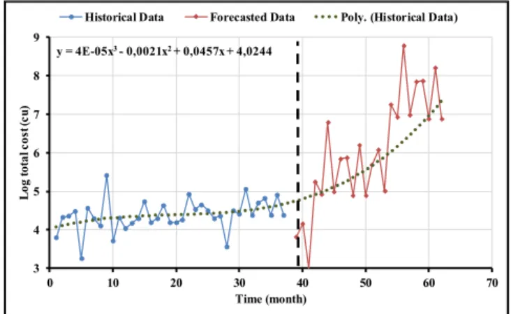
Figure 3 shows the results for ARIMA (2,1,1) for the TC with the polynomial trend curve. The forecasted data for the 24-month period do not seem to be in sync with the historical data before the vertical line or with the polynomial trend curve after the vertical line. The forecasted data are much higher than the historical and polynomial trends.

y = 4E-05x3_{- 0,0021x}2_{+ 0,0457x + 4,0244} 0 10 20 30 40 50 60 70 0 10 20 30 40 50 60 70 L og to ta lc os t( cu ) Time (month)

(3)

The results of ARIMA (2,0,3) are shown in Figure 4. In the figure, the forecasted data for the 24-month period seem to be in sync with the historical data before the vertical line and with the polynomial trend curve after the vertical line. Accordingly, these parameters are suitable for forecasting the TC data for this mining drilling rig.

Figure 4. ARIMA (2,0,3)

Overall, the forecasting using ARIMA (2,0,3) has better results than forecasting using the other ARIMA input parameters. We also find that the values of (p, d, q) affect the ARIMA forecasting, and the ARIMA (p, d, q) values are sensitive to the data type.

IV. CONCLUSION AND FUTURE WORK

The forecasting for our case study using the ARIMA model shows different forecasting abilities using different values of ARIMA parameters (p, d, q). The ARIMA parameters (p, d, q) are used in four different scenarios, one of which shows suitable forecasting. We find that the parameter values have a strong effect on the forecasting method. Therefore, these parameters need better estimation from the data for accurate forecasting. AI such as MOGA based on the ARIMA model could provide other possibilities for estimating the parameters (p ,d ,q) and improve data forecasting. The outcome of the MOGA based on the ARIMA model can be used to forecast data with a high level of accuracy, and the forecasted data can be used for life cycle cost analysis. For example, they can be used to estimate the optimal replacement time of the face drilling rig used in our case study.

ACKNOWLEDGMENT

The people at Boliden AB and Epiroc Rock Drills AB who helped in this research are gratefully acknowledged. The maintenance personnel and CMMS employees at Boliden AB who helped us in this research are also thanked for their support. In addition, we would like to extend our gratitude to Dr Ali Ismail Awad, Luleå University of Technology, Luleå, Sweden, for allowing us to use the computing facilities of the Information Security Laboratory to conduct the experiments in this study.

REFERENCES

[1] G.E. Box, G.M. Jenkins, G.C. Reinsel and G.M. Ljung, Time series analysis: forecasting and control, 4th_{ed, John Wiley &}

Sons, 2016.

[2] Y. Chen, B. Yang, J. Dong and A. Abraham, "Time-series forecasting using flexible neural tree model," Inf.Sci., vol. 174, October 2004, pp. 219-235.

[3] J.V. Hansen, J.B. Mcdonald, and R.D. Nelson, "Time Series Prediction With Genetic‐Algorithm Designed Neural Networks: An Empirical Comparison With Modern Statistical Models", Computational Intelligence, vol. 15, 1999, pp. 171-184.

[4] N.R. Herbst, N. Huber, S. Kounev and E. Amrehn, "Self adaptive workload classification and forecasting for proactive resource provisioning," Concurrency and computation: practice and experience, vol. 26, March 2014, pp. 2053-2078.

[5] D. Kwiatkowski, P.C. Phillips, P. Schmidt and Y. Shin, "Testing the null hypothesis of stationarity against the alternative of a unit root: How sure are we that economic time series have a unit root," J. of Econometrics, vol. 54, 1992, pp. 159-178.

[6] R.J. Hyndman and Y. Khandakar, Automatic time series for forecasting: the forecast package for R, Monash University, Department of Econometrics and Business Statistics, 2007.

[7] G.P. Zhang, "Time series forecasting using a hybrid ARIMA and neural network model," Neurocomputing, vol. 50, 2003, pp. 159-175.

[8] I. Hatzakis and D. Wallace, "Dynamic multi-objective optimization with evolutionary algorithms: a forward-looking approach," in Proceedings of the 8th annual conference on Genetic and evolutionary computation, July 2006, pp. 1201-1208.

[9] T. Vantuch and I. Zelinka, "Evolutionary based ARIMA models for stock price forecasting," in ISCS 2014: Interdisciplinary Symposium on Complex Systems, vol. 14, 2015, pp. 239-247. y = 4E-05x3_{- 0,0021x}2_{+ 0,0457x + 4,0244} 3 4 5 6 7 8 9 0 10 20 30 40 50 60 70 L og to ta lc os t( cu ) Time (month)