Policy Uncertainty Shocks in a Small Open Economy
Author: Jonathan Ahlén 901121
Spring 2019
Master Thesis in Finance, Advanced level, 30 credits Master’s programme in Finance
Örebro University, School of Business Supervisor: Pär Österholm
Abstract
Previous studies suggest that there is a significant correlation between economic policy uncertainty and macroeconomic variables such as GDP growth and unemployment rate. A commonly used tool in order to demonstrate this is by computing impulse response functions using vector autoregressive models. Some of the previous findings suggest that a shock in the US EPU index has a larger impact on Swedish GDP growth than a shock in the Swedish EPU index. The purpose of this study is to analyse if shocks in economic policy uncertainty in Sweden or the US have any impact on the Swedish real economy, and to determine whether the EPU indices can help forecast Swedish GDP growth. The impulse response functions in this study are in line with the results of previous research. However, the results of an out-of-sample forecast exercise show that the EPU indices do not help forecast Swedish GDP growth.
1
1. Introduction
Uncertainty appears to rapidly jump up after major economic and political shocks, such as the OPEC oil-price and supply shocks in the 70’s and 80’s, the events of September 11 in 2001, the fall of Lehman Brothers in 2008, the Greece bailout in 2011 and the Brexit referendum in 2016. For a long period of time economists have observed this pattern and measured the uncertainty and its impact on the real economy.1 Baker, Bloom & Davis (2013) developed a new index of economic policy uncertainty (EPU), by obtaining counts of newspaper coverage frequency that contained keywords pertaining to the economy, uncertainty and policy matters. The indices came to great use in the work area and enabled a range of future research. Stockhammar & Österholm (2016) showed by using the indices developed by Baker et al. (2013) that major shocks in economic policy uncertainty in the US, have a significant negative impact on Swedish GDP growth and other macroeconomic aggregates.
The purpose of this study is to analyse if shocks in economic policy uncertainty in Sweden or the US have any impact on the Swedish real economy, and to determine whether the variables can help forecast Swedish GDP growth. To fulfil the purpose, this study answers two questions. 1) Will shocks in the US or Swedish economic policy uncertainty impact the Swedish real economy? 2) Can economic policy uncertainty help forecast Swedish GDP growth?
Previous research has shown that monetary policy decisions have a major impact on a country’s economic future.2 Evidence of the relationship between shocks in the Swedish EPU and the Swedish real economy could help decision makers with expectations of future fluctuations in the economy.3 A variable that could help forecast economic growth could be of great importance to policymakers. Earlier work has been focusing on analysing EPU shocks in large open economies and the effect on macroeconomic or financial aggregate variables. Stockhammar & Österholm (2016) investigated the effects of US economic policy uncertainty on Swedish GDP growth using the EPU index of (Baker et al., 2013). They found that shocks to the economic policy uncertainty index have a significant negative effect on Swedish GDP growth. Some work has been done in the eurozone and on small open economies but to a lesser
1 See Bloom (2009) and Bachmann, Elstner & Sims (2010) for details.
2 See Friedman (1968), Bernanke & Gertler (1995), Clarida, Galí & Gertler (1998), Clarida, Galí & Gertler (2000)
Taylor (2014) for details.
2 extent. For example, Colombo (2013) investigated the effects of a US economic policy uncertainty shock on some macroeconomic aggregates in the eurozone, where the results showed that a shock to the US EPU leads to a statistically significant fall in the European inflation and industrial production. Armelius, Hull & Stenbacka Köhler (2017) constructed a Swedish EPU index by following the approach in (Baker et al., 2013). This opened for future research with Swedish economic policy uncertainty, that in turn enabled this study.
In order to analyse the relationship between the EPU indices and the Swedish real economy, vector autoregressive (VAR) models are estimated on the sample period 1993Q1 to 2018Q4. Using VAR models allow impulse response functions (IRF) to be computed which can be used to simulate shocks in economic policy uncertainty. Multiple model specifications are estimated in order to isolate the effects, generated by shocks in the Swedish or US EPU indices. An out-of-sample forecast exercise is conducted to examine whether the Swedish or US EPU indices can help forecast Swedish GDP growth. In order to carry through the forecast exercise, VAR models are estimated to generate forecasts with an eight-quarter horizon. The forecasts are then evaluated using different types of forecasting error measures and by conducting a Diebold-Mariano test.
By using a data sample that differs from previous research, this study contributes to the research area with an in-sample analysis of the relationship between Swedish economic policy uncertainty and the Swedish real economy. It also contributes with an out-of-sample forecast exercise, where the Swedish and US EPU indices are tested whether they could help forecast Swedish GDP growth.
The results from the IRF suggest that a one standard deviation shock to the Swedish EPU index delivers an impact on Swedish GDP growth, lowering the growth by 0.17 percentage points one quarter after the shock. However, a shock to the US EPU index delivers an impact on Swedish GDP growth, lowering the growth by 0.36 percentage points one quarter after the shock. These results suggest that the economic policy uncertainty in the US has a greater impact on the Swedish economy than the country’s domestic economic policy uncertainty. The IRF also suggests that a shock to either the Swedish or US EPU index increases the Swedish unemployment rate. However, this effect is not significant, although close to significant and shows a persistent pattern. The results from the out-of-sample forecast exercise suggest that neither the Swedish nor the US EPU indices help forecasting Swedish GDP growth.
3 The outline of this paper begins with a review of the previous literature in the work field of economic policy uncertainty. This is followed by a data chapter that describes how information has been collected and processed before and during this essay, as well as the problems regarding these methods. Subsequently, the empirical analysis is presented where the empirical framework and forecasting evaluation test are described. Finally, the results are presented which is followed by a discussion and conclusion of the work.
2. Previous Studies
Previous literature show that policy uncertainty in fiscal, monetary and regulatory policy have detrimental effects on the economy.4 Being able to measure economic policy uncertainty has proven to be very interesting for decision makers. Baker et al. (2013) developed new indices as a proxy to measure the economic policy uncertainty (EPU).5 The indices are based on newspaper coverage frequency, which offer distinct advantages compared to other policy uncertainty measures. These EPU indices have been evaluated by comparing them to other measures of uncertainty and policy uncertainty. According to Baker et al. (2016), the 30-day option-implied volatility in the S&P500 stock index (VIX) is an obvious comparison. It turns out that they often move in the same pattern with a correlation of 0.58, but sometimes also show a distinct variation. VIX reacts more strongly to events with a strong financial and stock market connection, such as the collapse of Lehman Brothers. In contrast, the EPU indices show stronger responses to events that involve major policy concerns that affect stock market volatility. Such as elections, political tax and government spending battles. Baker et al. (2016) described this as a proof-of-concept for their basic approach to construct a reasonable proxy for an important type of economic uncertainty, using frequency counts of newspaper articles. The newspaper-based indices can be extended to many countries and backwards in time. They can also be constructed at a daily frequency and easily be disaggregated into indices with specific categories. The indices are frequently used in the work field of policy uncertainty and its effects on macroeconomic variables. Despite the rapidly growing literature, the indices published by Baker et al. (2013) seem to have become a benchmark newspaper-based measure
4 See Friedman (1968), Rodrik (1991), Hassett and Metcalf (1999) for details.
5 Baker et al. published the indices as a working paper in 2013 which was later accepted in the Quarterly Journal
of Economics in 2016, hence the different references. However, there are some differences in the versions of the papers. The EPU indices have been updated and expanded, also there are some changes in the text. This means that it matters which index has been used and referred to, because it may affect the study.
4 of economic policy uncertainty.6 The relevance of this paper is of great importance to this study since it is the leading measure of economic policy uncertainty.
Another paper that has been of great importance is Armelius et al. (2017) who investigated the effects of shocks in Swedish EPU on various Swedish macroeconomic variables. By following the approach of Baker et al. (2013) the authors constructed a Swedish EPU index which is published and updated on (Economic Policy Uncertainty, 2019). They used a series of VAR’s and found that a one standard deviation shock to the Swedish EPU index, reduces Swedish GDP growth in the same quarter. However, a one standard deviation shock to the US or EU EPU indices showed a slower impact which arrived with a one quarter delay. This study uses the index published by Armelius et al. (2017) and conducts the in-sample analysis as this study, which makes the paper relevant for this study.
A study by Stockhammar & Österholm (2016) contributed with a lot of inspiration to the research area. This paper investigated the effects of US economic policy uncertainty on Swedish GDP growth using the EPU index developed by (Baker et al., 2013). By using impulse response functions from a Bayesian Vector Autoregressive (BVAR) model and spectral analysis, they found that shocks to the economic policy uncertainty index have a significant negative effect on Swedish GDP growth. According to the authors, their findings should prove useful to those who forecast and analyse the Swedish economy, or other similar small open economies. This line of work has also been done in the euro zone. Colombo (2013) investigated the effects of a US economic policy uncertainty shock on some macroeconomic aggregates in the euro area using several structural VAR’s. The findings in their study showed that a shock to the US EPU leads to a statistically significant fall in the European inflation and industrial production, which seems to be in line with results from other small open economies.
A well-known paper in this line of work is written by Bloom (2009) who analysed the impact of uncertainty shocks and not particularly economic policy uncertainty shocks. The author presented a new structural framework where the model is used to simulate a macro uncertainty shock, which produces a drop and rebound in the aggregate output and unemployment. According to the author, the reason for the drop in the output and unemployment is due to higher uncertainty, which causes firms to temporarily pause their hiring and investments. This makes the productivity growth fall because of the pause in activity, which causes reallocation across units to freeze. The simulated impacts of uncertainty shocks are then compared to VAR
5 estimations on actual data. The results showed a good match in both timing and magnitude which greatly contributed to the work field and enabled a range of future research. This paper is relevant to this study, as it highlights the effect of what shocks in uncertainty may have on the real economy and opens for further research with more specified issues.
There are some papers with relevance to this study that investigated the EPU indices ability to forecast financial and macro-aggregated variables. Brogaard & Detzel (2015) used the US EPU index created by Baker et al. (2013) in order to forecast log excess market returns. The study resulted in two interesting findings. They found that economic policy uncertainty is positively associated with an increase in forecasted three-month abnormal returns. They also found that among the Fama French25 portfolios formed on size and momentum returns, the portfolio with the greatest EPU beta underperformed the portfolio with the lowest EPU beta.7 Even when controlling for exposure to the Carhart four factors as well as implied and realized volatility.8 These findings suggests that EPU is an economically important risk factor for equities.
Investigating the EPU indices ability to forecast financial and macro-aggregated variables has been examined before but to a lesser extent. Kurasawa (2017) estimated a probit model to predict the recession probability in the US, using economic policy uncertainty indices developed by (Baker et al., 2013). He found the EPU indices to be relatively useful as predictors of recession but is sceptical about the indices being a proxy for economic policy uncertainty. On the other hand, according to Junttila & Vataja (2018) the inclusion of EPU measures for the US, UK or overall European economies, improves the forecasting ability of models based on standard financial market information. With disagreeing findings in previous studies, it makes it more interesting to examine whether the Swedish or the US EPU index can help forecast the Swedish real economy.
This research area is wide and there are some interesting studies that investigated general policy uncertainty and its effect on the economy. For example, Grafinkel & Glazer (1994) investigated if electoral uncertainty causes economic fluctuations using a different approach.9 They analysed the data on wage contracts and identified a tendency that economic agents postpone contract negotiations until after the election. This evidence is interesting as political uncertainty affects corporate performance. Another paper that used the EPU indices developed by Baker et al. (2013) but in a different approach is written by (Karnizova and Jiaxiong, 2014). Their study
7 For information about the Fama French asset pricing model see (Fama & French, 1993). 8 For information about the extension of the Fama French model, see (Carhart, 1997). 9 For more studies like this, see (Durnev, 2010).
6 used probit recession forecasting models to assess the ability of EPU indices to predict future US recessions. The model specifications include financial variables such as interest rate spreads, stock market volatility and stock returns in addition to the EPU indices. The in-sample and out-of-sample analysis results suggested, that the EPU indices are statistically and economically significant in forecasting recessions at horizons beyond five quarters.
3. Data
This chapter presents the data and some timeseries properties tests.
This study uses quarterly data from 1993Q1 to 2018Q4 for the analysis. The reason why this period started at 1993Q1, is because Sweden went from fixed to floating exchange rate and inflation targeting in 1992, which caused some fluctuations in the economy. Both EPU indices will be used as non-dependant variables. The US EPU index is calculated by Baker et al. (2016) and the Swedish EPU index is calculated by Armelius et al. (2017) following the same approach as in (Baker et al., 2013). Updates of the indices are available at Economic Policy Uncertainty (2019) from where the EPU data have been collected. Swedish GDP growth will be used as a dependent variable and the data have been collected from the (Statistics Sweden, 2019). The data are available in quarterly frequency and with various calculation methods as well as seasonal and calendar-adjustments. This study uses data calculated by the production approach and with seasonal and calendar adjustments. Swedish unemployment rate (UER) will be used as both dependent and non-dependent variable and the data have been collected from the (National Institute of Economic Research Sweden, 2019). The Swedish 3-month Treasury Bill rate (T-Bill) will be used as a non-dependant variable and the data have been collected from the (Swedish Central Bank, 2019). The model specifications will be presented in section four. Quarterly observations have been generated by taking the averages of the original monthly observations for the EPU, T-Bill and unemployment series. Table 3.1 presents descriptive statistics for all variables.
7
Table 3.1. Descriptive statistics.
Swedish EPU Swedish GDP Swedish T-Bill Swedish UER US EPU
Mean 96.338 0.6365 2.8240 7.8618 113.13 Median 97.394 0.7000 2.7099 7.6762 103.93 Maximum 159.93 2.4000 9.6476 11.397 235.08 Minimum 57.287 -3.7000 -0.7786 5.7049 52.089 Std. Dev. 18.753 0.8882 2.6706 1.5451 37.306 Skewness 0.3251 -1.6248 0.6971 0.6721 0.7045 Kurtosis 3.2812 8.6679 2.9031 2.4832 2.9899 Jarque-Bera 2.1749 184.97 8.4649 8.9874 8.6032 J-B p-values 0.3371 0.0000 0.0145 0.0112 0.0135 Observations 104 104 104 104 104
Notes: Quarterly data are used with a sample period of 1993Q1 to 2018Q4. The Swedish GDP enters as a growth rate. The p-values presented are from the Jarque-Bera test.
Notice that this sample period includes high treasury bill rates as well as negative treasury bill rates. It also includes periods where the EPU indices seem to have fluctuated a bit when comparing the maximum and minimum values with the mean, especially for the US EPU index. The sample consists of 104 observations for all series. Table 3.1 also presents values of the Jarque-Bera test which is a goodness-of-fit test of the sample data, that shows whether the data have the skewness and kurtosis matching a normal distribution. If the value is far from zero, it signals that the data does not follow a normal distribution. The sample includes recessions as well as one of the toughest financial crisis in history, which can explain the minimum value of Swedish GDP growth and the high value of the Swedish unemployment rate in 2009. In order to get a better overview of the sample, the series for each variable are plotted in Figure 3.1.
8
Figure 3.1. Data plot.
Notes: Quarterly data are used with a sample period of 1993Q1 to 2018Q4. Years are shown on the horizontal axis and values (for the EPU indices) or percent of each series on the vertical axis. The EPU indices are included in levels, GDP enters as growth rate, Unemployment rate (UER) in per cent and Treasury bill rate (T-Bill) in per cent.
By interpreting the Swedish EPU index in Figure 3.1, it seems that the index value increases during the Swedish financial crises in the early-mid 1990s. It also increases during the Russian financial crisis in 1998, coinciding when the Stockholm stock exchange also experienced its biggest fall since 1900. The EPU index tends not only to increase during financial crises but also during other crises such as the Dot-com bubble and the 9/11 terrorist attacks in 2001. It also has some local peaks during the financial crisis in 2008 and the eurozone crisis in 2011. Comparing the Swedish EPU index with the Swedish GDP growth suggests a negative relationship between the two variables. As the EPU index increases, GDP growth tends to move in the opposite direction and vice versa. By observing the data plot, it seems that this period
40 60 80 100 120 140 160 180 94 96 98 00 02 04 06 08 10 12 14 16 18 Swedish EPU -4 -3 -2 -1 0 1 2 3 94 96 98 00 02 04 06 08 10 12 14 16 18 Swedish GDP -2 0 2 4 6 8 10 94 96 98 00 02 04 06 08 10 12 14 16 18 Swedish T-Bill 40 80 120 160 200 240 94 96 98 00 02 04 06 08 10 12 14 16 18 US EPU 5 6 7 8 9 10 11 12 94 96 98 00 02 04 06 08 10 12 14 16 18 Swedish UER
9 captures a pattern that looks like a negative trend in both Swedish unemployment rate and the Swedish treasury bill rate.10
In the economical long run perspective, the Swedish treasury bill rate should be mean reverting, as the central bank uses monetary policy instruments and the government fiscal policy to maintain long-term economic growth with a stable price level.11 There is an ongoing debate regarding the unemployment rate being stationary or not, which is still not clear.12
The economic policy uncertainty indices tend to follow the Swedish GDP growth variable quite well. Uncertainty appears to rapidly jump up in times of major economic and political crises and decrease in less turbulent times. Visual inspection indicate that economic policy uncertainty should be treated as a non-trending series that might exhibit mean level shifts.
In addition to plotting the series, unit root tests are conducted to show whether the series are stationary or not. Two common tests for unit roots are Augmented Dickey-Fuller (ADF) and Kwiatkowski-Phillips-Schmidt-Shin (KPSS) both of which are used in this study.13 The ADF tests the null hypothesis that a unit root is present in a time series sample unlike the KPSS test, which is used for testing the null hypothesis that an observable time series is stationary around a deterministic trend or level. Sometimes it could help making the series stationary by taking the first difference of the series and then test it again for unit root. The ADF tests have been conducted with a constant for series at level, and when testing the first difference of the series the test is conducted without a constant. Regarding the KPSS test, all series have been conducted with a constant, both at level and in first difference. The test statistics of the unit root test results are presented in Table 3.2.
10 Correlations between the variables are shown in Table A.1 in the Appendix.
11 The Swedish central bank uses monetary policy to keep inflation low and stable. This in turn affects the
treasury bill rates as they move together (Riksbanken, 2019).
12 See Gustavsson & Österholm (2011) and Cevik & Dibooglu (2013) for details.
13 See Dickey & Fuller (1976) and Kwiatkowski, Phillips, Schmidt & Shin (1992) for details about the unit root
10
Table 3.2. Results from unit root tests on individual series.
Variable series ADF KPSS
SweEPUi -3.007″ 0.307 ∆SweEPUi -9.547‴ 0.129 SweGDPi -5.498‴ 0.134 ∆SweGDPi -12.69‴ 0.071 SweTBilli -2.088′ 1.112‴ ∆SweTBilli -4.810‴ 0.114 SweUERi -2.381 0.483″ ∆SweUERi -5.940‴ 0.069 US EPUi -4.248‴ 0.546″ ∆US EPUi -11.08‴ 0.093
Notes: ‴ Significant at the 1% level. ″ Significant at the 5% level. ′ Significant at the 10% level. Taking the first difference of the series is indicated with a delta. Swedish GDP is measured in terms of growth.
Notice that all series except the Swedish unemployment rate are stationary on different significance levels, given the test results from the unit root tests on this sample. However, taking the first difference of every series makes all series stationary on a one per cent significant level. The data sample is not optimal and can be criticized in various ways. To begin with, this study does not use real-time data as it is much less publicly available and sometimes not even stored but replaced with revised data. However, it is important to highlight the benefits of using real-time data. For example, real-real-time data could improve the out-of-sample analysis when using Swedish GDP growth data in real-time.14 The EPU indices are calculated backwards in time and based on newspaper coverage published in real-time. The preferred comparison would then be to use Swedish GDP growth data in real-time, in order to increase the results of the out-of-sample exercise. The out-of-sample length is also to be taken into consideration. It is often better to have a bigger sample with more observations, especially if the study uses quarterly or annual data frequency. Furthermore, the chosen period involves one of the biggest financial crisis in history, and with a small sample the results could get misleading. As mentioned earlier, this sample period captures patterns in some variable series that could be interpreted as trends, but normally are stationary when looking at a bigger sample. The relationship between the EPU index and the Swedish unemployment rate could have been analysed with monthly frequency instead of quarterly data. Which might have given a different result and a different interpretation. The reason behind converting all data series into quarterly frequency is to interpret the effects in quarters after the initiated shocks in EPU. The sources of data are public authorities and are considered credible and of good quality. The data for the EPU index is
14 Orphanides (2001) highlights the importance of using real-time data by demonstrating that real-time policy
11 supported by previous research and is considered an appropriate index as a proxy for economic policy uncertainty.
4. Empirical Model
This section introduces the method that is used to answer the addressed research question. The empirical framework is based on vector autoregressive (VAR) models with univariate, different bivariate and multivariate model specifications. The usage of VAR models consistently appears in several studies to estimate statistical relationships between the EPU indices and other variables of interest. VAR models are useful statistical devices for evaluating alternative macroeconomic models according to (Sims, 1980).15 The reason for using a VAR model compared to a univariate time series model is quite clear. By extending the univariate autoregressive model with vectors, it enables cross-variable dynamics. Each variable is related not only to its own past, but also to the past of all the other variables in the system. Another type of multivariate interaction that univariate models lack, is that the disturbances may be correlated. So that when one equation is shocked, the other equations will typically be shocked as well (Diebold, 2006). A general case of a VAR(p) with n variables is
𝑦1,𝑡 = 𝑐1+ ƒ111 𝑦 1,𝑡−1+ ⋯ + ƒ1𝑛1 𝑦𝑛,𝑡−1+ ⋯ + ƒ11 𝑝 𝑦1,𝑡−𝑝+ ⋯ + ƒ1𝑛𝑝 𝑦𝑛,𝑡−𝑝+ 𝜀1𝑡, ⋮ ⋮ 𝑦𝑛,𝑡 = 𝑐𝑛+ ƒ1𝑛1𝑦1,𝑡−1+ ⋯ + ƒ𝑛𝑛1 𝑦𝑛,𝑡−1+ ⋯ + ƒ𝑛1 𝑝 𝑦,𝑡−𝑝+ ⋯ + ƒ𝑛𝑛𝑝 𝑦𝑛,𝑡−𝑝+ 𝜀𝑛𝑡. (4.1)
The method estimates n different equations using ordinary least squares (OLS) where each equation regresses the dependent variable on p lags of itself and p lags of every other variable. The disturbance variance-covariance structure of the VAR(p) is given by
𝜀𝑖,𝑡~ 𝑊𝑁(0, 𝜎𝑖2), ⋯ 𝜀𝑗,𝑡~ 𝑊𝑁(0, 𝜎𝑗2), 𝐶𝑜𝑣(𝜀𝑖,𝑡, 𝜀𝑗,𝑡) = 𝜎𝑖,𝑗.
(4.2)
The disturbances i,j are uncorrelated if 𝜎𝑖,𝑗 equals zero. One of the main assumptions of standard VARs models is stationarity of the data. The unit root test results presented in Table 3.2 suggests
15 Christiano (2012) offers an interesting discussion on the original paper by Sims (1980) and highlight interesting
12 that all series except the Swedish unemployment rate are stationary. As mentioned earlier, there is an ongoing debate whether unemployment rate is mean reverting or in presence of unit root. This study follows the assumption that the unemployment rate is mean reverting. Hence, no variable will be used as in first difference, but at level.
The importance of determination of lag lengths has proven to be of great importance. Braun and Mittnik (1993) showed that VAR estimates whose lag length differs from the true lag length are inconsistent, as are IRF derived from the VAR estimates. Selecting a higher order of lag length than the true lag length, may result in overfitting and causes an increase in the forecast MAE. Choosing a lower order of lag length than the true lag length often generates autocorrelated errors (Lütkepohl, 1993).
In order to determine the lag length in the VAR system, the Akaike Information Criterion (AIC) is used. The lag order p is selected so that the AIC is minimized.16 The model specifications for the in-sample and out-of-sample analysis, together with the test results from the AIC, are presented in Table 5.1. Some of the out-of-sample model specifications are not used in the in-sample analysis and vice versa. This is shown by using two different columns in Table 5.1.
Table 5.1. In-sample and Out-of-sample model specifications.
Variables
In-Sample
Out-of-Sample
AIC
Model 1 SWE GDP growth No Yes 5 lags
Model 2 SWE GDP growth, SWE EPU index Yes Yes 5 lags
Model 3 SWE GDP growth, US EPU index Yes Yes 5 lags
Model 4 SWE GDP growth, SWE UER, SWE T-Bill No Yes 2 lags
Model 5 SWE GDP growth, SWE UER, SWE T-Bill, SWE EPU index Yes Yes 2 lags Model 6 SWE GDP growth, SWE UER, SWE T-Bill, US EPU index Yes Yes 2 lags
Model 7 SWE UER, SWE EPU index Yes No 4 lags
Model 8 SWE UER, US EPU index Yes No 3 lags
Notes: The test results of the Akaike Information Criterion (AIC) suggested the following lag lengths on the sample period of 1993Q1 to 2018Q4.
The impulse response function is a device that makes the dynamic properties of VAR models understandable, which could be of interest to forecasters. For example, the function answers
13 the question, how does a one standard deviation shock in 𝜀𝑖,𝑡 effect 𝑦𝑗,𝑡+ℎ now and in the future for all various combinations of n?
In order to recover orthogonal shocks, first a VAR model is fitted to the Swedish and US data from the first quarter of 1993 to the last quarter of 2018.17 Second, impulse response functions are calculated using Cholesky decomposition with the following ordering; GDP growth, EPU index or unemployment rate, EPU index in the bivariate cases.18 In the fourvariate model specifications the following ordering is applied; Unemployment rate, GDP growth, EPU index and T-bill. It also applies to the trivariate model specification where the EPU index is excluded.19
According to Armelius et al. (2017) the Swedish newspapers provide a considerable amount of coverage from the US, which means that the Swedish EPU index is expected to contain much information associated with the US EPU index.20 However, one could argue that a better measure of idiosyncratic shocks in Sweden and the US is the orthogonal component of each of these countries EPU series, with respect to other countries, EPU series. This approach would greatly reduce the variation in the series related to idiosyncratic events occurring the same year (Biljanovska, Grigoli & Hengge, 2017). Hence, this study uses the same approach as (Armelius et al., 2017).
In addition to examine whether shocks in the EPU indices have any effect on the Swedish real economy, an out-of-sample forecast exercise will be conducted to determine whether the Swedish or US EPU indices can help forecast GDP growth in Sweden. This is performed by estimating VAR model specifications on half of the data sample to generate forecasts of Swedish GDP growth. A forecast horizon of eight quarters is chosen in order to capture the
17 Two vectors in an inner products space are orthogonal if their inner product is zero. A critique that has been
raised against forecast error impulse responses is that the underlying shocks are not likely to occur in isolation if the errors are instantaneously correlated, that is, if the sum of the errors are not diagonal. Therefore, orthogonal innovations are preferred in an impulse response analysis. One way to get this is by using Cholesky decomposition (Krätzig & Lütkepohl, 2004).
18 The Cholesky decomposition is a decomposition of a self-adjoint matrix into the product of a lower triangular
matrix and its conjugate transpose. 𝐴 = [𝐿][𝐿]𝑇 where A is symmetric and its own transpose. A is decomposed
into the product of [𝐿] and the conjugate transpose [𝐿]𝑇.
19 The ordering matters when using Cholesky decomposition as the variables are placed in the decreasing order of
exogeneity. The variables are ordered by using economic theory. In the order where one variable is most likely to influence the other, but not the other way around. Hence, unemployment rate is more likely to influence GDP growth, EPU and at last Three-month treasury bill rate, than the other way around and so on. This ordering gave the most significant results. Other ordering has also been tried, which generates similar but not identical results.
20 The correlation between the Swedish EPU index and US EPU index is only 0.22, which indicates that there
should not be any problems regarding multicollinearity. A correlation matrix is presented in Table A.1 in the Appendix.
14 lagged effects of monetary policy decisions on the economy.21 When the first forecast is conducted, the same VAR model specification is re-estimated but with an extension of the data sample by one period, and a new forecast is conducted. This exercise is repeated until the forecasts cover the latter half of the sample period.
This will be conducted with the six different model specifications presented in Table 5.1. The models include the variables Swedish or US EPU index, Swedish unemployment rate, GDP growth and treasury bill rate. However, the models will differ in such fashion that some of the models will exclude the EPU index. This is due to being able to carry out a forecast evaluation. The forecast evaluation consists of comparing different evaluation measures. The measures are based on calculations of forecasts errors. When evaluating these measures, the smallest possible forecast error is preferred. Mean absolute error (MAE), mean square error (MSE) and root mean square error (RMSE) are commonly used measures.22 In addition to these calculations, a Diebold-Mariano test based on the MSE is conducted. The calculations of the forecast evaluation measures are presented in the following equations.
The mean absolute error is calculated by summing the absolute values of the forecast errors at time t+h, and divide it with n, where n is the forecasting periods and h the forecast horizon,
Instead of calculating the absolute value of the forecast errors, they can be squared,
𝑀𝑆𝐸 =1
𝑛∑ 𝑒𝑡+ℎ|𝑡
2 .
𝑛
𝑡=1 (4.4)
By taking the square root of the MSE, it is possible to interpret the values in the original format,
𝑅𝑀𝑆𝐸 = √1
𝑛∑ 𝑒𝑡+ℎ2 |𝑡.
𝑛
𝑡=1
(4.5)
These evaluation measures are similar and do not differ that much in the calculations. The obvious approach is to select the forecast that has the smallest error measurement based on one
21 See Freidman (1961) for details.
22 The measurements are discussed in Hyndman & Koehler (2006) and applied in papers such as Österholm (2008)
and (Croushore & Stark, 2001).
𝑀𝐴𝐸 =1 𝑛∑|𝑒𝑡+ℎ|𝑡| 𝑛 𝑡=1 . (4.3)
15 of the measures described in Equation 4.3-4.5. However, to determine whether there is a significant loss-differential between the forecast errors, a Diebold-Mariano test is conducted.23 First, 𝑑𝑖 is denoted as the loss-differential between the forecast errors of model one, 𝑒𝑖2 and the forecast errors of model two, 𝑟𝑖2,
𝑑𝑖= 𝑒𝑖2− 𝑟𝑖2. (4.6)
Secondly, the mean is calculated of the loss-differential 𝑑𝑖,
𝑑 = 1 𝑛∑ 𝑑𝑖 𝑛 𝑖=1 . (4.7)
In order to construct the Diebold-Mariano test statistic, the autocovariance of 𝑑𝑖 is estimated,
𝛾𝑘 = 1 𝑛 ∑ (𝑑𝑖− 𝑑̅)(𝑑𝑖−𝑘− 𝑑̅) 𝑛 𝑖=𝑘+1 . (4.8) The DM test follows asymptotically a standard normal distribution with 𝐷𝑀~ 𝑁(0,1),
𝐷𝑀 = 𝑑
√[𝛾0+ 2 ∑ℎ−1𝑘=1𝛾𝑘]
𝑛
(4.9)
Under the null hypothesis of a zero expected loss differential, there is a significant difference between the forecasts if the value of the DM statistic is larger than the critical z-value. Where the z-value is the two tailed critical value for the standard normal distribution.
23 The usefulness of the Diebold-Mariano (DM) test has been discussed recently. The DM test was intended for
comparing forecasts and remains useful in that regard. However, many of the ensuring literature uses DM-type tests for comparing models. See Diebold (2015) for details and discussion on the topic.
16
5. Results
In this section the results are presented. At first, the in-sample relationship between the Swedish and US EPU indices and the proxy variables for the Swedish real economy, Swedish GDP growth and Swedish unemployment rate is analysed. This is presented by using impulse response functions computed on estimated bivariate VAR specifications. Secondly, as some of the effect can be explained by other variables, the VAR model specifications are extended with more variables to isolate the effect of the Swedish GDP growth in the EPU index.24 Finally, an out-of-sample forecast exercise is conducted to see if the Swedish and US EPU indices can help forecast Swedish GDP growth. The out-of-sample results are presented by plotting the forecasts, the evaluations measures and by conduction a Diebold-Mariano test.
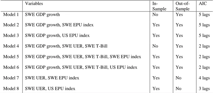
Figure 5.1 shows how Swedish GDP growth and unemployment rate responds to a one standard deviation shock in domestic EPU index, together with the associated ± two standard error confidence intervals.25
Figure 5.1. Impulse Responses to Swedish EPU Index.
Notes: Each IRF is generated for a separate bivariate VAR. Quarterly data are used with a sample period of 1993Q1 to 2018Q4. Percentage points are shown on the vertical axis and quarters are shown on the horizontal axis. Estimated values in solid blue line and ± 2SE in black dotted line.
The impulse response functions from the bivariate VAR model specifications suggests that a shock to the Swedish EPU index has a significant negative effect on the Swedish GDP growth. Notice that the largest impact on Swedish GDP growth occurs one quarter after the shock to the Swedish EPU index, with a drop of 0.17 percentage points. The IRF also suggests that a shock to the Swedish EPU index increases the Swedish unemployment rate. This effect is however not significant, although close to significant in the first and second quarter.
24 Complete output of all impulse response functions can be found in the Appendix Figure A.1 to Figure A.6. 25 The standard deviation for Swedish EPU index is 18.75.
-0.4 0.0 0.4 0.8 1.2 1 2 3 4 5 6 7 8 9 10 Swedish GDP -.2 .0 .2 .4 .6 1 2 3 4 5 6 7 8 9 10 Swedish UER
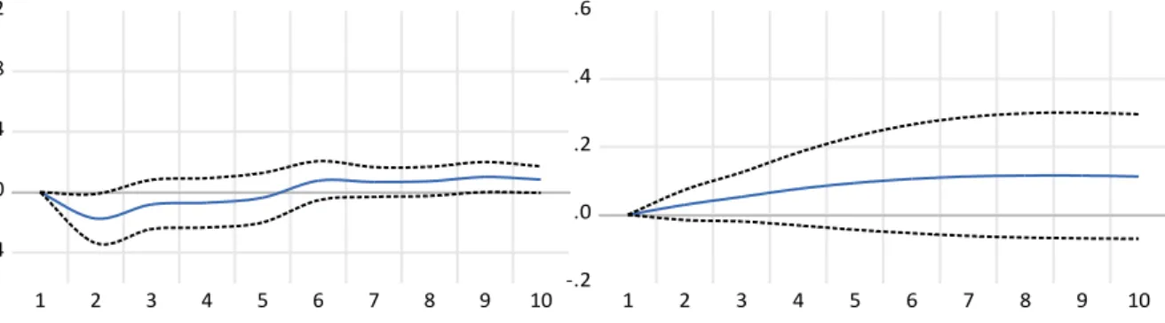
17 Figure 5.2 shows how Swedish GDP growth and unemployment rate responds to a one standard deviation shock in US EPU index, together with the associated ± two standard error confidence intervals.26
Figure 5.2. Impulse Responses to US EPU Index.
Notes: Each IRF is computed using a separate bivariate VAR. Quarterly data are used with a sample period of 1993Q1 to 2018Q4. Percentage points are shown on the vertical axis and quarters are shown on the horizontal axis. Estimated values in solid blue line and ± 2SE in black dotted line.
The impulse response functions from the bivariate VAR model specifications suggest that a shock to the US EPU index has a significant negative effect on the Swedish GDP growth. According to the IRF the largest impact on the Swedish GDP growth can be observed one quarter after the shock to the foreign EPU index. Notice that the GDP growth in Sweden drops by 0.36 percentage points one quarter after the shock in the US EPU index, and by 0.19 percentage points four quarters after the shock to the US EPU index. Comparing the results one quarter after the shock with the response to a one standard deviation shock in the domestic EPU index, it seems that US economic policy uncertainty has a bigger impact by almost 0.2 percentage points on the Swedish GDP growth. However, the impulse responses show no significant results in the Swedish unemployment rate to a shock in the US EPU index.
Some of the effects in Swedish GDP growth can be explained by other variables. By extending the bivariate specification to a fourvariate specification it is possible to isolate the effect generated by shocks in the Swedish or US EPU indices. The VAR model is extended by including Swedish GDP growth, unemployment rate and Swedish three-month treasury bill rate in addition to the EPU index.
26 The standard deviation for US EPU index is 37.31.
-0.4 0.0 0.4 0.8 1.2 1 2 3 4 5 6 7 8 9 10 Swedish GDP -.2 .0 .2 .4 .6 1 2 3 4 5 6 7 8 9 10 Swedish UER
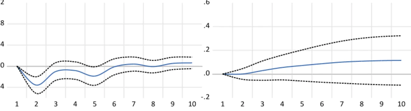
18 Figure 5.3 presents the results from the multivariate model specification including the Swedish EPU index. The impulse responses show how Swedish GDP growth, unemployment rate, three-month treasury bill rate and the Swedish EPU index, responds to a one standard deviation shock in domestic EPU index, together with the associated ± two standard error confidence intervals for each response variable.
Figure 5.3. Impulse Responses for Swedish EPU Index.
Notes: Each IRF is computed using a multivariate VAR. Quarterly data are used with a sample period of 1993Q1 to 2018Q4. Percentage points are shown on the vertical axis and quarters are shown on the horizontal axis. Estimated values in solid blue line and ± 2SE in black dotted line.
In line with the results from the bivariate specifications. The impulse response function of the multivariate VAR model specification suggests that a shock in Swedish EPU index tends to have a negative effect on Swedish GDP growth, and lower the Swedish three-month treasury bill rate. The effect on the Swedish unemployment rate is statistically insignificant but close to significant in the first and second quarter as recognized in the bivariate specification. These results suggest that the index developed by Armelius et al. (2017) captures an effect as a proxy for the economic policy uncertainty in Sweden quite well.
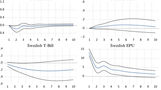
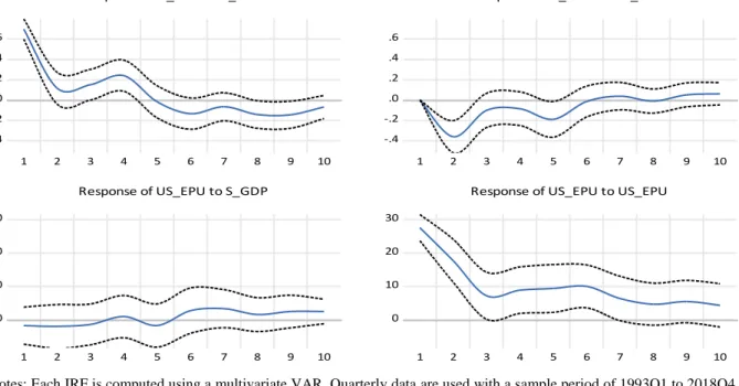
Figure 5.4 shows how Swedish GDP growth, unemployment rate, three-month treasury bill rate and the US EPU index, responds to a one standard deviation shock in the US EPU index, together with the associated ± two standard error confidence intervals for each response variable. -0.4 0.0 0.4 0.8 1.2 1 2 3 4 5 6 7 8 9 10 Swedish GDP -.2 .0 .2 .4 .6 1 2 3 4 5 6 7 8 9 10 Swedish UER 0 5 10 15 1 2 3 4 5 6 7 8 9 10 Swedish EPU -.6 -.4 -.2 .0 .2 .4 1 2 3 4 5 6 7 8 9 10 Swedish T-Bill
19
Figure 5.4. Impulse Responses for US EPU Index.
Notes: Each IRF is computed using a multivariate VAR. Quarterly data are used with a sample period of 1993Q1 to 2018Q4. Percentage points are shown on the vertical axis and quarters are shown on the horizontal axis. Estimated values in solid blue line and ± 2SE in black dotted line.
The impulse response functions from the multivariate VAR model specifications including the US EPU index, suggests that a shock to the US EPU index has a significant negative effect on the Swedish GDP growth. The impact on Swedish GDP growth is slightly lower in the first quarter, compared to the bivariate model specification. On the other hand, the unemployment rate is even closer to being significant in the extended model specification. The impulse response function also suggests that a one standard deviation shock in the US EPU index lowers the Swedish T-bill rate by 0.2 percentage points.
In order to analyse the forecasting ability of the Swedish EPU index created by Armelius et al. (2017) and the US EPU index created by Baker et al. (2016), an out-of-sample forecast exercise was conducted using different model specifications. The models are estimated using 50 percent of the sample to generate forecasts with an eight-quarter horizon. For each created forecast, the model is re-estimated with one period extension of the sample. This continues as a recursive forecast to cover the full sample period, that is to the last quarter of 2016.
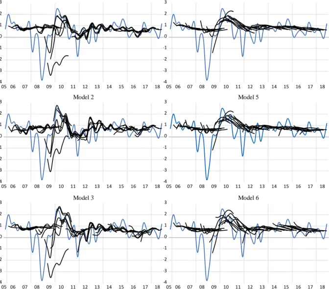
Six different model specifications were used in the exercise. Model 1 is a univariate AR specification with only Swedish GDP growth as variable. Model 2 is a bivariate VAR specification with Swedish GDP growth and Swedish EPU index as variables. Model 3 is a
-.2 .0 .2 .4 .6 1 2 3 4 5 6 7 8 9 10 Swedish UER -.4 .0 .4 .8 1 2 3 4 5 6 7 8 9 10 Swedish GDP 0 10 20 30 1 2 3 4 5 6 7 8 9 10 US EPU -.6 -.4 -.2 .0 .2 .4 1 2 3 4 5 6 7 8 9 10 Swedish T-Bill
20 bivariate VAR specification with Swedish GDP growth and US EPU index as variables. Model 4 is a trivariate VAR specification with Swedish GDP growth, Swedish Unemployment rate and Swedish Three-month Treasury bill rate as variables. Model 5 is a fourvariate VAR specification with Swedish GDP growth, Swedish Unemployment rate, Swedish Three-month Treasury bill rate and Swedish EPU index as variables. Model 6 is a fourvariate VAR specification with Swedish GDP growth, Swedish Unemployment rate, Swedish Three-month Treasury bill rate and US EPU index as variables.
Figure 5.5 shows the out-of-sample recursive forecasts of Swedish GDP growth. Actuals are shown in blue and forecast values in black.
Figure 5.5. Out-of-sample forecast exercise.
Notes: Out-of-sample forecasts computed on sample ranging from 1993Q1 to 2005Q4/2016Q4. Percent on the vertical axis and time on the horizontal axis.
-4 -3 -2 -1 0 1 2 3 05 06 07 08 09 10 11 12 13 14 15 16 17 18 Model 6 -4 -3 -2 -1 0 1 2 3 05 06 07 08 09 10 11 12 13 14 15 16 17 18 Model 5 -4 -3 -2 -1 0 1 2 3 05 06 07 08 09 10 11 12 13 14 15 16 17 18 Model 4 -4 -3 -2 -1 0 1 2 3 05 06 07 08 09 10 11 12 13 14 15 16 17 18 Model 3 -4 -3 -2 -1 0 1 2 3 05 06 07 08 09 10 11 12 13 14 15 16 17 18 Model 2 -4 -3 -2 -1 0 1 2 3 05 06 07 08 09 10 11 12 13 14 15 16 17 18 Model 1
21 The forecasts seem to predict Swedish GDP growth quite well except during the financial crisis of 2008-2009. There are however some visual differences when comparing the models. The trivariate-and fourvariate model specifications, seem to predict the Swedish GDP growth more accurately than the univariate and bivariate model specifications. In order to determine if the Swedish and US EPU indices could help improve forecasting the Swedish GDP growth, forecasting errors have been calculated which are presented in Table 5.1.
Table 5.1. Results from out-of-sample forecast exercise.
Horizon Model 1 Model 2 Model 3
MAE MSE RMSE MAE MSE RMSE MAE MSE RMSE
1 0,707 1.142 1.069 0,739 1,219 1,104 0,662 0.979 0.989 2 0,704 1.298 1.139 0,706 1,247 1,117 0,691 1.295 1.138 3 0,829 1.646 1.283 0,791 1,387 1,178 0,843 1.699 1.303 4 0,813 1.776 1.333 0,790 1,536 1,240 0,770 1.733 1.316 5 0,813 1.763 1.328 0,790 1,541 1,241 0,822 1.841 1.357 6 0,811 1.530 1.237 0,757 1,295 1,138 0,828 1.623 1.274 7 0,801 1.525 1.235 0,797 1,351 1,162 0,843 1.607 1.268 8 0,771 1.353 1.163 0,760 1,276 1,130 0,756 1.309 1.144
Horizon Model 4 Model 5 Model 6
MAE MSE RMSE MAE MSE RMSE MAE MSE RMSE
1 0,759 1.342 1.158 0,795 1.386 1.177 0,810 1.358 1.165 2 0,698 1.175 1.084 0,706 1.190 1.091 0,689 1.144 1.070 3 0,711 1.211 1.101 0,693 1.183 1.088 0,671 1.176 1.084 4 0,724 1.247 1.117 0,724 1.237 1.112 0,710 1.252 1.119 5 0,672 1.190 1.091 0,665 1.182 1.087 0,650 1.172 1.082 6 0,714 1.248 1.117 0,706 1.245 1.116 0,712 1.249 1.117 7 0,722 1.249 1.117 0,713 1.250 1.118 0,715 1.251 1.118 8 0,752 1.319 1.148 0,750 1.311 1.145 0,750 1.336 1.156
Notes: Out-of-sample forecast errors computed on sample ranging from 1993Q1 to 2005Q4/2016Q4. Forecast horizons are one to eight quarters. Model 1 is a univariate AR specification with only Swedish GDP growth as variable. Model 2 is a bivariate VAR specification with Swedish GDP growth and Swedish EPU index as variables. Model 3 is a bivariate VAR specification with Swedish GDP growth and US EPU index as variables. Model 4 is a trivariate VAR specification with Swedish GDP growth, Swedish Unemployment rate and Swedish Three-month Treasury bill rate as variables. Model 5 is a fourvariate VAR specification with Swedish GDP growth, Swedish Unemployment rate, Swedish Three-month Treasury bill rate and Swedish EPU index as variables. Model 6 is a fourvariate VAR specification with Swedish GDP growth, Swedish Unemployment rate, Swedish Three-month Treasury bill rate and US EPU index as variables.
Notice that there are differences when comparing the forecast mean absolute errors and root mean square errors. The multivariate models seem to outperform the univariate and bivariate models on most of the forecast horizons. Model 5 and Model 6 seem to perform more accurately by comparing the forecast MAE and RMSE, which are the models including the EPU indices. It is however important to evaluate these forecast errors and to have statistical evidence that there is a difference between the forecast errors. Conducting a Diebold-Mariano test ensures if the loss differential is zero, or different from zero, between the models that contain the EPU
22 index and the models that exclude the EPU index. This test has been conducted testing the loss differential between Model 1 and 2, Model 1 and 3, Model 4 and 5, Model 4 and 6. The results are presented in Table 5.2.
Table 5.2. Results from Diebold-Mariano test based on squared values of forecast errors. Horizon Model 1 vs. Model 2 Model 1 vs. Model 3 Model 4 vs. Model 5 Model 4 vs. Model 6
1 0.308 0.173 0.518 0.845 2 0.594 0.946 0.659 0.514 3 0.341 0.665 -0.996 0.374 4 0.298 0.638 -0.564 0.861 5 0.261 0.235 -1.113 0.335 6 0.295 0.120 -0.437 0.994 7 0.328 0.331 0.181 0.966 8 0.204 0.390 -0.769 0.713
Notes: Out-of-sample forecast errors computed on sample ranging from 1993Q1 to 2005Q4/2016Q4. Forecast horizons are one to eight quarters. ‴ Significant at the 1% level. ″ Significant at the 5% level. ′ Significant at the 10% level. Model 1 is a univariate AR specification with only Swedish GDP growth as variable. Model 2 is a bivariate VAR specification with Swedish GDP growth and Swedish EPU index as variables. Model 3 is a bivariate VAR specification with Swedish GDP growth and US EPU index as variables. Model 4 is a trivariate VAR specification with Swedish GDP growth, Swedish Unemployment rate and Swedish Three-month Treasury bill rate as variables. Model 5 is a fourvariate VAR specification with Swedish GDP growth, Swedish Unemployment rate, Swedish Three-month Treasury bill rate and Swedish EPU index as variables. Model 6 is a fourvariate VAR specification with Swedish GDP growth, Swedish Unemployment rate, Swedish Three-month Treasury bill rate and US EPU index as variables.
The results of the Diebold-Mariano test show that there is none t-statistic that is statistically significant at a one, five or ten per cent level, which means that there is no statistical evidence that there is a difference between the squared forecasting errors for any of the specified models.
23
6. Discussion
The in-sample results from the impulse response functions are in line with the results of what Armelius et al. (2017) found. However, there are some small differences in size of the effects when shocks in the EPU indices are simulated. The largest effect on the Swedish GDP growth arrives one quarter after the shock in Swedish EPU. This differs from Armelius et al. (2017) where the impact arrived in the same quarter as the shock, and then dissipated over the following quarters. But comparing a shock to the US EPU, the largest impact on Swedish GDP growth arrives with a one quarter delay, which is in line with (Armelius et al. 2017). On the other hand, comparing this study’s results with Stockhammar & Österholm (2016), the results turned out to have larger differences. A shock to the US EPU index delivers a larger drop in the Swedish GDP growth suggested by the IRF in this study. These differences could be explained by the fact that there is a difference between using a VAR model and a BVAR model. Comparing the results of this study with the results that Colombo (2013) found in the eurozone, they seem to be leaning towards the same conclusion, but with different macroeconomic variables used. Colombo (2013) found that a shock to the US EPU leads to a statistically significant fall in the European inflation and industrial production. It seems that economic policy uncertainty in large open economies such as the US impacts the real economy, not only in Sweden but in other small open economies in Europe. Based on the results of this study, both US and Swedish economic policy uncertainty seem have effects on Swedish GDP growth. As mentioned by Stockhammar & Österholm (2016) and by Bloom (2009), the reason for this could be that companies pause their hiring and investments, and that households lower their consumptions, in times of higher economic policy uncertainty.
The out-of-sample forecast exercise was conducted in order to test whether the Swedish or the US EPU indices could help forecast the Swedish GDP growth. The forecasting evaluation measures MAE and RMSE showed that, by adding the EPU indices lower the forecast errors and improves the Swedish GDP growth forecast. However, the results from the Diebold-Mariano tests showed that the null hypothesis of a zero expected loss differential could not be rejected at any of the significance levels in any forecast horizon. Comparing these results with previous literature is difficult, since the research question whether the EPU indices could help forecast GDP growth has not been investigated in a broader context. Brogaard & Detzel (2015) used the US EPU index created by Baker et al. (2013) in order to forecast log excess market returns. Where they found that economic policy uncertainty is positively associated with an
24 increase in forecasted three-month abnormal returns. It seems that the indices can be used to help forecast some macro or financial variables to some extent, but not when forecasting Swedish GDP growth with the Swedish EPU index. If the EPU indices could be useful when forecasting a variable, it could be worth pointing out how often the indices are updated because it might reduce the usefulness of using the indices in practice. It is possible to get the US EPU index in daily frequency, but this is not publicly available for Sweden yet. The problem with this could be that if economic policy uncertainty would rapidly increase in the beginning of a month, the index is not calculated and published until the period is over. In that case, decision makers have already lost several weeks of valuable time that could have been used for evaluation. For example, had there been a rapid increase of economic policy uncertainty, they would not have been able to act based on the information that an evaluation would have given. It would have been interesting to see the Swedish EPU index on daily frequency, as it enables researching the relationship on financial variables on a day to day basis.
7. Conclusion
The purpose of this study is to analyse if shocks in economic policy uncertainty in Sweden or the US have any impact on the Swedish real economy, and to determine whether the variable can help forecast Swedish GDP growth. This purpose has been fulfilled by answering the following questions. 1) Will shocks in the US or Swedish economic policy uncertainty impact the Swedish real economy? 2) Can economic policy uncertainty help forecast Swedish GDP growth?
The results from a one standard deviation shock in the Swedish EPU index suggests that the Swedish GDP growth will drop by 0.17 percentage points in the first quarter. Comparing these results with the results from a one standard deviation shock in the US EPU index, the impulse response functions suggests that the Swedish GDP growth will drop by almost 0.36 percentage points. This indicates that economic policy uncertainty in the US has a larger effect on the Swedish real economy than the domestic economic policy uncertainty in Sweden. The results from the bivariate model specifications where unemployment rate was used as a proxy for the real economy in Sweden, showed no statistical significance on the effects. The results from the multivariate model specifications showed a slightly different effect on the Swedish GDP growth and unemployment rate when shocking the EPU indices. The IRF from the multivariate model
25 specification suggest that a one standard deviation shock in the Swedish EPU index lowers the Swedish GDP growth by 0.18 percentage points. Which is slightly higher than the effect in the bivariate case. On the other hand, the IRF from the multivariate model specification including the US EPU index, suggest that a one standard deviation shock in the US EPU index lower the Swedish GDP growth by 0.31 percentage points. This means that the effect in Swedish GDP growth is lower in the multivariate model specification, compared to the bivariate model specification.
The forecasting evaluation measurements showed, that the model specifications that include EPU indices seem to outperform the other model specifications by looking at the mean absolute errors and root mean squared errors. This is an indication that the EPU indices could help forecast the Swedish GDP growth, but it is not enough to conclude that the indices improve Swedish GDP growth forecasts. To ensure statistical evidence of a difference between the forecast errors, a Diebold-Mariano test was conducted. The result of the test showed that the null hypothesis of a zero expected loss differential could not be rejected on any of the horizons for any of the models forecasting errors that was tested.
To conclude this study. The usage of the indices published by Baker et al. (2016) and Armelius et al. (2017) as a proxy for economic policy uncertainty, showed a statistically significant in-sample relationship between the indices and the Swedish GDP growth. However, neither of these indices could be used out-of-sample to help forecast the Swedish GDP growth.
Some improvements could have been made to this study. The usage of real-time data could improve the out-of-sample forecast results. Also, an extension of the data sample or an extension of the VAR model specifications including other macroeconomic variables, could have resulted in a different outcome. The research question could have also been answered by using other models or extended models. Such as Bayesian VAR, that has been used by (Stockhammar & Österholm, 2016). Despite the significant results in the in-sample analysis, one should be aware that the indices are not direct measures of economic policy uncertainty but based solely on newspaper coverages.
A question for future research could be if the EPU indices could help forecast other macro or financial variables in different countries. Or if the Swedish EPU index could help forecast the Swedish GDP growth with a Bayesian approach.
References
Akaike, H. (1973). Information Theory and an Extension of the Maximum Likelihood Principle.
Proceeding of the Second International Symposium on Information Theory, pp. 267-281.
Akaike, H. (1974). A new look at the statistical model identification. IEEE Transactions on
Automatic Control, 19(6), pp. 716-723.
Alexopoulos, M. & Cohen, J. (2015). The Power of Print: Uncertainty Shocks, Markets, and the Economy. International Review of Economics and Finance, 40, pp. 8-28.
Armelius, H., Hull, I. & Stenbacka Köhler, H. (2017). The Timing of Uncertainty Shocks in a Small Open Economy. Economics Letters, 155, pp. 31-34.
Bachmann, R., Elstner, S. & Sims, E. R. (2010). Uncertainty and Economic Activity: Evidence from Business Survey Data. American Economic Journal: Macroeconomics, 5(2), pp. 217-249. Baker, S.R., Bloom, N. & Davis S.J. (2013). Measuring Economic Policy Uncertainty. Chicago
Booth Research Paper, 13(2).
Baker, S.R., Bloom, N. & Davis S.J. (2016). Measuring Economic Policy Uncertainty. The
Quarterly Journal of Economic, 131(4), pp. 1593-1636.
Bernanke, B.S. & Gertler, M. (1995). Inside the Black Box: The Credit Channel of Monetary Policy Transmission. Journal of Economic Perspectives, 9(4), pp. 27-48.
Biljanovska, N., Grigoli, F. & Hengge, M. (2017). Fear Thy Neighbor: Spillover from Economic Policy Uncertainty. International Monetary Fund, Working paper 17(240).
Bloom, N. (2009). The Impact of Uncertainty Shocks. Econometrica, 77(3), pp. 623-685. Braun, P. & Mittnik, S. (1993). Misspecifications in vector autoregressions and their effects on impulse responses and variance decompositions. Journal of Econometric, 59(3), pp. 319-341. Brogaard, J. & Detzel, A.L. (2015). The Asset Pricing Implications of Government Economic Policy Uncertainty. Management Science, 61(1).
Carhart, M.M. (1997). On persistence in Mutual Fund Performance. The Journal of Finance, 52(1), pp. 57-82.
Cevik, E.I. & Dibooglu, S. (2013). Persistence and non-linearity in the US unemployment: A regime-switching approach. Economic Systems, 37, pp. 61-68.
Clarida, R., Galí, J. & Gertler, M. (1998). Monetary policy rules in practice: Some international evidence. 42(6), pp. 1033-1067.
Clarida, R., Galí, J. & Gertler, M. (2000). Monetary Policy Rules and Macroeconomic Stability: Evidence and Some Theory. The Quarterly Journal of Economics, 115(1), pp. 147-180. Colombo, V. (2013). Economic policy uncertainty in the US: Does it matter for the Euro area?
Economics Letters, 121, pp. 39-42.
Christiano, L.J. (2012). Christopher a. Sims and Vector Autoregressions. The Scandinavian
Journal of Economics, 114(4), pp. 1082-1104.
Croushore, D. & Stark, T. (2001). A real-time data set for macroeconomists. Journal of
Econometrics, 105, pp. 111-130.
Dickey, D.A. & Fuller, W.A. (1976). Distribution of the Estimators for Autoregressive Time Series with a Unit Root. Journal of the American Statistical Association, 74(366a).
Diebold, F.X. (2006). Elements of Forecasting. 4th Edition. South-Western College Pub. Diebold, F.X. (2015). Comparing Predictive Accuracy, Twenty Years Later: A Personal Perspective on the Use and Abuse of Diebold Mariano Tests. Journal of Business & Economic
Statistics, 33(1).
Durnev, A. (2010). The Real Effects of Political Uncertainty: Elections and Investment Sensitivity to Stock Prices. SSRN Electronic Journal.
Economic Policy Uncertainty. (2019). Data collected for the EPU index. http://www.policyuncertainty.com/index.html [2019-03-04].
Fama, E.F. & French, K.R. (1993). A five-factor asset pricing model. Journal of Financial
Economics, 33(1), pp. 3-56.
Freidman, M. (1961). The Lag in Effect of Monetary Policy. Journal of Political Economy, 69(5), pp. 447-466.
Friedman, M. (1968). The Role of Monetary Policy. American Economic Review, 58(1), pp. 1-17.
Garfinkel, M.R. & Glazer, A. (1994). Does Electoral Uncertainty Cause Economic Fluctuations? American Economic Review, 84(2), pp. 169-173.
Gentzkow, M. & Shapiro, J.M. (2010). What Drives Media Slant? Evidence from US Daily Newspapers. Econometrica, 78(1), pp. 35-71.
Gustavsson, M. & Österholm, P. (2011). Mean reversion in the US unemployment rate – evidence from bootstrapped out-of-sample forecasts. Applied Economics Letters, 18(7), pp. 643-646.
Hasset, K. & Metcalf, G.E. (1999). Investment with Uncertain Tax Policy: Does Random Tax Policy Discourage Investment? Economic Journal, 109(457), pp. 372-393.
Hoberg, G. & Phillips, G. (2010). Product Market Synergies and Competition in Mergers and Acquisitions: A Text-Based Analysis. Review of Financial Studies, 23(1), pp. 3773-3811. Hyndman, R.J. & Koehler, A.B. (2006). Another look at measures of forecast accuracy.
International Journal of Forecasting, 22(4), pp. 679-688.
Junttila, J. & Vataja, J. (2018). Economic Policy Uncertainty Effects for Forecasting Future Real Economic Activity. Economic Systems, 42(4), pp. 569-583.
Karnizova, L. & Jiaxiong, L. (2014). Economic policy uncertainty, financial markets and probability of US recessions. Economic Letters, 125, pp. 261-265.
Krätzig, M. & Lütkepohl, H. (2004). Applied Time Series Econometrics. New York; Cambridge
University Press.
Kurasawa, K. (2017). Forecasting US recession with the economic policy uncertainty indexes of policy categories. Economics and Business Letters, 6(4), pp. 100-109.
Kwiatkowski, D., Phillips, P.C.B., Schmidt, P. & Shin, Y. (1992). Testing the Null Hypothesis of Stationarity Against the Alternative of a Unit Root. Journal of Econometrics, 54, pp. 159-178.
Lütkepohl, H. (1993). New Introduction to Multiple Time Series Analysis. New York, USA: Springer.
National Institute of Economic Research Sweden. (2019). Data collected for Swedish unemployment rate.
http://www.konj.se/english.html [2019-03-05].
Orphanides, A. (2001). Monetary Policy Rules Based on Real-Time Data. American Economic
Riksbanken. (2018). What is monetary policy?
https://www.riksbank.se/en-gb/monetary-policy/what-is-monetary-policy/ [2019-06-05]. Rodrik, K. (1991). Policy Uncertainty and Private Investment. Journal of Development
Economics, 36(2), pp. 229-242.
Sims, C.A. (1980). Macroeconomics and Reality. Econometrica, 48(1), pp. 1-48. Statistics Sweden. (2019). Data collected for Swedish GDP growth.
http://www.scb.se/en/finding-statistics/ [2019-03-04].
Stockhammar, P. & Österholm, P. (2016). Effects of US policy uncertainty on Swedish GDP growth. Empirical Economics, 50(2), pp. 443-462.
Swedish Central Bank. (2019). Data collected for Swedish 3-month Treasury Bill rate.
https://www.riksbank.se/en-gb/statistics/search-interest--exchange-rates/ [2019-03-06].
Taylor, J. B. (2014). The Role of Policy in the Great Recession and the Weak Recovery.
American Economic Review, 104(5), pp 61-66.
Österholm, P. (2008). Can Forecasting Performance be Improved by Considering the Steady State? An Application to Swedish Inflation and Interest Rate. Journal of Forecasting, 27, pp. 41-51.
Appendix
Figure A.1 to Figure A.6 presents the complete outputs of the impulse response functions generated from estimated VAR models. Each IRF show the response of a one standard deviation shock using Cholesky decomposition. The responses are presented with the associated ± two standard error confidence intervals. The IRF in Figure A.1 is generated from an estimated bivariate VAR model specification including Swedish EPU index and Swedish GDP growth. The IRF in Figure A.2 is generated from an estimated bivariate VAR model specification including the US EPU index and Swedish GDP growth. The IRF in Figure A.3 is generated from an estimated bivariate VAR model specification including Swedish EPU index and Swedish unemployment rate. The IRF in Figure A.4 is generated from an estimated bivariate VAR model specification including US EPU index and Swedish unemployment rate. The IRF in Figure A.5 is generated from an estimated fourvariate VAR model specification including Swedish EPU index, Swedish GDP growth, Swedish Unemployment rate and Swedish three-month T-bill rate. The IRF in Figure A.6 is generated from an estimated fourvariate VAR model specification including the US EPU index, Swedish GDP growth, Swedish Unemployment rate and Swedish three-month T-bill rate.
Figure A.1. Impulse response functions of bivariate VAR model specification including Swedish EPU index.
Notes: Each IRF is computed using a multivariate VAR. Quarterly data are used with a sample period of 1993Q1 to 2018Q4. Percentage points are shown on the vertical axis and quarters are shown on the horizontal axis. Estimated values in solid blue line and ± 2SE in black dotted line. Swedish GDP growth is abbreviated with S_GDP and the Swedish EPU index is abbreviated with S_EPU. -.2 .0 .2 .4 .6 .8 1 2 3 4 5 6 7 8 9 10 Response of S_GDP to S_GDP -.4 -.2 .0 .2 .4 .6 .8 1 2 3 4 5 6 7 8 9 10 Response of S_GDP to S_EPU -4 0 4 8 12 1 2 3 4 5 6 7 8 9 10 Response of S_EPU to S_GDP -4 0 4 8 12 1 2 3 4 5 6 7 8 9 10
Response of S_EPU to S_EPU
Figure A.2. Impulse response functions of bivariate VAR model specification including US EPU index.
Notes: Each IRF is computed using a multivariate VAR. Quarterly data are used with a sample period of 1993Q1 to 2018Q4. Percentage points are shown on the vertical axis and quarters are shown on the horizontal axis. Estimated values in solid blue line and ± 2SE in black dotted line. Swedish GDP growth is abbreviated with S_GDP and the US EPU index is abbreviated with US_EPU.
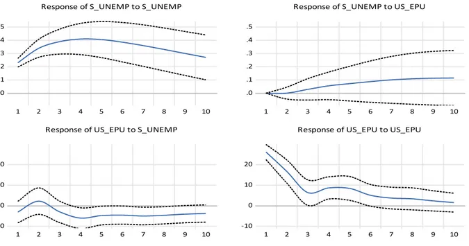
Figure A.3. Impulse response functions of bivariate VAR model specification including Swedish EPU index.
Notes: Each IRF is computed using a multivariate VAR. Quarterly data are used with a sample period of 1993Q1 to 2018Q4. Percentage points are shown on the vertical axis and quarters are shown on the horizontal axis. Estimated values in solid blue line and ± 2SE in black dotted line. Swedish unemployment rate is abbreviated with S_UNEMP and the Swedish EPU index is abbreviated with S_EPU.
-.4 -.2 .0 .2 .4 .6 1 2 3 4 5 6 7 8 9 10 Response of S_GDP to S_GDP -.4 -.2 .0 .2 .4 .6 1 2 3 4 5 6 7 8 9 10 Response of S_GDP to US_EPU 0 10 20 30 1 2 3 4 5 6 7 8 9 10 Response of US_EPU to S_GDP 0 10 20 30 1 2 3 4 5 6 7 8 9 10
Response of US_EPU to US_EPU
Response to Cholesky One S.D. (d.f. adjusted) Innovations ± 2 S.E.
.0 .1 .2 .3 .4 .5 1 2 3 4 5 6 7 8 9 10
Response of S_UNEMP to S_UNEMP
.0 .1 .2 .3 .4 .5 1 2 3 4 5 6 7 8 9 10
Response of S_UNEMP to S_EPU
0 4 8 12
1 2 3 4 5 6 7 8 9 10
Response of S_EPU to S_UNEMP
0 4 8 12
1 2 3 4 5 6 7 8 9 10
Response of S_EPU to S_EPU