Experiences from the Swedish Value of Time study

W

s

t

t

d

d

s

c

d

t

Expe

We provide

study, with

travel behav

these enable

distribution.

discussed, in

savings. Fur

characteristi

differentiate

transport app

weighted

tre for Tra 100 44 Sto eden w.cts.kth.s

eriences f

Maria Börj

Jonas Elia

a synthesis

focus on w

viour. We s

e a better

. The influe

ncluding th

rther, we sh

ics, discuss

ed in apprai

praisal.

Value of

d cost-benef

from the

esson, Roy

asson, Roya

s of results a

what is relev

summarize r

understandi

ence of the

he problems

how how th

s in what

sal, and pro

time, appra

fit analysis.

Swedish

al Institute

al Institute o

and insights

vant for tran

recent econ

ing and ide

e sign and

of loss ave

he value of t

dimension

ovide recom

aisal, cost-b

h Value o

of Technolo

of Technolo

s from the S

nsport appra

nometric adv

entification

size of cha

ersion and t

time depend

ns the valu

mmended va

benefit anal

of Time s

ogy (KTH)

gy (KTH)

Swedish Va

aisal and un

vances, and

of the val

anges is est

the value of

ds on trip a

ue of time

alues for use

lysis, travel

study

alue of Time

nderstanding

d show how

lue of time

timated and

f small time

and traveller

should be

e in applied

l behaviour

e

g

w

e

d

e

r

e

d

r,

1

1

INTRODUCTION

The value of travel time savings (VTTS) is central in transport economics and transport policy. Still, it is a remarkably elusive concept, since the VTTS varies across situations and individuals. The VTTS varies both with socioeconomic characteristics, such as income, family situation and employment status, and with trip-related characteristics such as time of day, trip purpose and comfort aspects. Even after controlling for such observable factors, there is a considerable ”unexplained” or ”idiosyncratic” variation in the VTTS.

In recent years, new econometric methods have made it possible to gain a deeper understanding of the variation in the VTTS, both the part related to observable characteristics and the idiosyncratic part (Fosgerau, 2006; Fosgerau, 2007). The VTTS is often estimated on experimental data, usually hypothetical experiments such as stated choice surveys. The recent methodological advances have also resulted in a better understanding of how VTTS estimates are affected by the design of the choice experiment and by its short-term nature, and also how these phenomena can be removed to reveal the reference-free VTTS that is usually the relevant entity for use in transport appraisal.

The purpose of this paper is to present results and experiences from the Swedish Value of Time study, carried out in Sweden during 2008, comprising trips with car, bus or train of all lengths and purposes except employer’s business. This study is the first where the methodological advances have been used to successfully estimate the mean of the VTTS distribution. Previous attempts, using data from the Danish Value of Time study, highlighted the demands put on the data by the presence of heterogeneity in the valuations. In particular, the data needs to support identification of a sufficient range of the valuation distribution. The Swedish study was explicitly designed to meet these data requirements, giving unprecedented opportunities to understand VTTS variation. The purpose of this paper is not to present the details of the econometric methodology – there are companion papers that do that (Börjesson, Fosgerau, & Algers, 2012a; Börjesson, Fosgerau, & Algers, 2012b; Börjesson, 2010a). Instead, the focus of this paper is to summarize and discuss the results and insights, and give a synthesis relevant for applied transport appraisal and for understanding travel behaviour.

Section 2 summarizes the econometric advances enabling the subsequent analyse. Non-parametric methods provide insights concerning the identification of the VTTS distribution and the appropriate parametric model specification (see Fosgerau (2006) and Börjesson et al. (2012a)). Parametric methods make it possible to include covariates that capture effects of socioeconomics variables and reference dependence. Section 3 discusses the influence of “size effects” and “sign effects” in stated choice experiments that are due to the short-run nature of the experimental setting. Size effects include the problem of valuing small time savings, while sign effects include phenomena such as loss aversion. Recent methodological advances have made it possible to uncover how the VTTS is affected by size and sign effects, and also how to

2

remove them to some extent, to capture the long-run, reference-free VTTS that is relevant for virtually all policy purposes, Failure to control for these phenomena may cause severe bias of estimation results: results will depend critically on the stated choice design, in a way that is impossible to detect without looking for it.

Section 4 presents estimation results, showing how the VTTS varies with the characteristics of the trip and the traveller. In section 5, we discuss in which dimensions the VTTS can and should be differentiated in applied appraisal, and present our recommended values for use in appraisal. In particular, we discuss how income effects on the VTTS should be treated, and show how the VTTS changes if income effects are removed. Section 6 concludes.

2

THE ECONOMETRICS OF VTTS ESTIMATION

2.1

Non-parametric estimation

Assume that respondents choose between two trip alternatives differing with respect to travel cost and travel time. Denote the variables (c1,t1) and (c2,t2). Let y be an

indicator variable which is 1 if the respondent chooses alternative 1 and 0 otherwise. Let the individual-specific VTTS be denoted by W, and introduce = ( − ) (⁄ − ). Assume that the experimental design is such that V>0 for all choices, that is, in each choice a slower, cheaper alternative is compared with a faster, more expensive one; we will assume that the alternatives are numbered such that c2>c1

and t2<t1. We will call V the bid, since it is the trade-off value of travel time.

Each respondent will choose the slow alternative if W<V, i.e. = 1 < 1_{. Assuming}

that the respondent reveals if her VTTS is higher or lower than the bid in each stated choice, the cumulative distribution function (CDF) of the VTTS can be estimated non-parametrically using local constant regression2 _{(the method is explained in detail in}

Fosgerau (2007)). The idea is to plot the bids against the share of respondents accepting each bid – in other words, the share of respondents with VTTS less than the bid – thereby obtaining an estimate of the CDF of the VTTS. The strength of this method is that it is possible to estimate the distribution of the value of time (and hence its moments) without any assumptions about error structure or parameterisations. Figure 1 shows a non-parametric estimate of the CDF of the VTTS distribution for drivers. (As will be explained below, the VTTS depends on how the stated choice question relates to the reference trip; the figure shows the willingness-to-pay distribution.)

In the figure, the right-hand tail of the CDF does not differ significantly from 1, implying that most of the right-hand tail is identified. In the Danish value of time study, a significant part of VTTS distribution was left unsupported because a significant part of the respondents were seemingly non-traders, always choosing the most expensive alternative (Fosgerau, 2006). The Swedish study used the bid range 1-50 €/h, more than twice the range in the Danish data, which was sufficient for eliminating virtually all non-traders (only 1-2 per cent of the respondents accepted the highest bids).

Since a significant part of the VTTS distribution was not supported in the Danish data, the mean value of time could not be estimated. This is a potential problem for all types of valuation studies using random parameters, but it is often “hidden”. It is possible to

1 _{1{x>y} is defined to take the value 1 if x>y and 0 otherwise.} 2

3

estimate the parameters of any assumed parameter distribution even if the distribution has only partial support and hence cannot be completely identified. The mean and other moments may, however, depend strongly on the tail of the distribution, which is not supported by the data! If the problem is not recognized, it is easy to fall into the trap of estimating a full distribution using only the range supported by the data, and then arrive at results which in effect depend on the parts of the distribution that are extrapolated outside the data range. This could be a serious bias, and it should be stressed that it is possible to commit this error without noticing it.

Figure 1: Non-parametric estimate of the WTP distribution: mean and 95 percent confidence interval.

2.2

Parametric estimation

Non-parametric estimates are sufficient if one is content with estimating the distribution of the VTTS, and thereby it’s mean, variance and other moments. To introduce covariates, however, one must specify a parametric model. There are several reasons for exploring how the VTTS depends on covariates:

1. The choices are to some extent influenced by characteristics of the experiment, such as the size and sign of the time differences between the alternatives. These “experimental artefacts” exist in the short-term experimental setting, but are usually not relevant for the use of the value of time, such as appraisal of long-term policy measures or investments. Introducing them as covariates makes it possible to remove these effects, at least to some extent.

2. Understanding how the VTTS varies with characteristics of the trip and the traveller gives a better understanding of travel behaviour, and makes it possible to extrapolate the VTTS to new situations, without having to make new surveys. 3. One may want to remove the influence of certain factors, most commonly income. As we will show, there is also a considerable difference between the VTTS of rural and urban areas. Introducing covariates provides a possibility to remove the effect of these differences. These issues are discussed in section 5. 4. Introducing covariates enables a better identification of the tail of the

distribution, as will be explained below. 0 0.1 0.2 0.3 0.4 0.5 0.6 0.7 0.8 0.9 1 0 100 200 300 400 500

WTP

4

The traditional way to estimate the VTTS parametrically is to assume that individuals have utility functions of the form

= + (1)

where c is travel cost, t is travel time, and α and β are parameters to be estimated. The parameters α and β can be interpreted as marginal utilities (MU) of money and time, respectively, while the ratio β/α is the value of time, i.e. the marginal rate of substitution (MRS) between time and money. We can estimate α and β by applying the model

= 1 + > + + (2)

If is taken to be logistically distributed, a logit model results. Note that this model has three degrees of freedom (α, β and the variance of ε; with rational respondents and a true model, E(ε)=0), but only two of these can be estimated. Intuitively, the two degrees of freedom stem from two sources: one is the trade-off between cost and time (the value of time), and the other is the variance of the error term (the extent of unexplained variation in the data). The standard way to identify the model is to fix the variance of the error term. To account for heterogeneity in the value of time, α and β can be assumed to follow some random distributions, and the parameters of these distributions can be estimated.

An alternative model is obtained by rearranging the terms in the definition of y above

= 1 < + ̃ , (3)

To distinguish the two specifications, we will call the former “estimating in MU-space” and the latter “estimating in MRS-space”. Both models are consistent with random utility maximization: the only difference between them is the specification of the error term. We have ̃ = / ( − ), so either of the models can be seen as variant of the other but allowing for a specific form of heteroskedasticity in the error term (Var( ) ∼ Var( ̃) ∗ ( − ) ).

The choice of model is an empirical matter. To get indications of which model is most consistent with data, non-parametric estimation in the (∆t,∆c)-space can be applied to visualize the response surfaces in the data (Fosgerau, 2007). Börjesson et al. (2012a) show that the MRS space model is more consistent with the Swedish VTTS data.

Estimating in MRS space has a practical advantage over the MU space formulation: it facilitates the introduction of covariates. When estimating in MU space, covariates can be introduced by interacting covariates with different parameters in different ways. It often becomes confusing and even combinatorially infeasible to test many covariates simultaneously. Specifying the model in MRS space, however, makes it easier to explore how the VTTS depends on various covariates simultaneously, as will be demonstrated below.

To define the parametric model, the response variable y is still defined as = 1 < , where W is the individual-specific VTTS and V is the bid. Taking logs and adding an iid standard logistic error term ε, we have:

5

The parameter μ is a scale parameter. Then, parameterize W as

= exp( * + +) (5)

where β is a vector of parameters, x is a vector of covariates, and δ is a constant. δ is assumed to be constant for each individual but normally distributed in the population. This formulation ensures that W is positive, while the ranges of β and δ are unrestricted. The assumption that δ is individual-specific and varies randomly in the population takes care of the correlation of the unobserved heterogeneity arising from repeated observations of the same individuals. An essential assumption is that x and δ are independent, implying that the distribution of the VTTS is unaffected by a shift in x. The assumption that δ is normal implies that the VTTS is assumed to be lognormally distributed across the population, once the influence of the covariates has been controlled for. The assumption about the distribution of δ is important and can be tested using Biogeme (Fosgerau & Bierlaire, 2007; Bierlaire, 2008; Bierlaire, 2003). Using this test it is found that the VTTS distributions in the present study are indeed very close to lognormal. Interestingly, the value of time studies in Denmark and Norway also indicate that the VTTS distribution is lognormal or close to lognormal3

(Fosgerau, 2007; Ramjerdi, Flügel, Samstad, & Killi, 2010).

Because the VTTS distribution is highly skewed, it is crucial to introduce the random parameter δ in the MRS space specification. Without this, the mean VTTS will typically be severely underestimated in the MRS space specification. Attempts at estimating in MRS space were hence doomed to fail before the advent of robust methodology and software for random-parameters estimation. For example, estimation in the MRS space was explored in the previous the Swedish VTTS study (Dillén & Algers, 1998), but without applying any mixing distribution since the necessary econometric software and theory was not available at the time. This MRS specification was abandoned since it resulted in an unrealistically low VTTS4_.

As listed above, there are several reasons for introducing covariates in the model. One less obvious reason is that it enables a better identification of the tail of the VTTS distribution. To see this, rewrite the model as = 1 + < "#$ − * + %/& . While the VTTS distribution can only be identified over the range of "#$ in the non-parametric estimation, the parameterization means that the VTTS distribution can be identified over range of "#$ − *, which is a wider range since the covariates * add to the variation of "#$ .

3

DATA

The data was collected through two surveys carried out in 2007 and 2008. The 2007 survey was an identical replication of the Swedish 1994 VTTS study relating to drivers (Dillén & Algers, 1998). Drivers were recruited using number plate registration, and subsequently interviewed over telephone. The 2008 survey comprised several modes: car, long and short distance train and bus. Car drivers were recruited using a random

3

In the Danish data, the VTTS true distribution could not be estimated, since the bid range was too small. It was, however, obvious that the distribution was skewed.

4 _{Recent MRS space estimation applying the error term as specified in this section and the VTTS data} from 1994 results in considerably higher mean VTTS within a more normal range.

6

sample from the population register. The respondent was asked to list all car trips on a specified day, from which one trip was randomly selected. Selection probabilities were higher for long distance trips to get a sufficient number of such trips. For the public transport modes, respondents were recruited on board by collecting passengers’ addresses and telephone numbers. Respondents could choose to respond to the questionnaire by Internet or by a call-back telephone interview, to avoid a potential selection bias and low response rate due to differences in Internet access. A full scale follow up survey by telephone was carried out. For car, the total response rate was 59 percent5_{, while the response rate for public transport varied between 70-75 percent.}

The total number of respondents was for car 1440; regional bus, 950; regional train, 931; long distance bus, 699; long distance train 561. A description of the 2007 survey, including the experimental design, can be found in Börjesson et al. (2012b), a description of the 2008 car study in Börjesson et al. (2012a) and description of the 2008 public transport study in Börjesson (2010b).

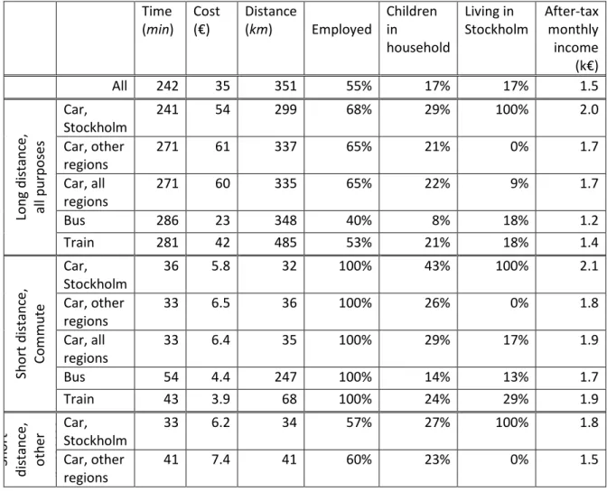
Table 1 shows the sample statistics for different travel segments weighted with trip distances (to get the sample representative of what would be found on an average link, which is the VTTS relevant for most appraisal purposes).

Table 1: Sample statistics weighted with trip distance.

Time (min) Cost (€) Distance (km) Employed Children in household Living in Stockholm After-tax monthly income (k€) All 242 35 351 55% 17% 17% 1.5 Lo n g d is ta n ce , a ll p u rp o se s Car, Stockholm 241 54 299 68% 29% 100% 2.0 Car, other regions 271 61 337 65% 21% 0% 1.7 Car, all regions 271 60 335 65% 22% 9% 1.7 Bus 286 23 348 40% 8% 18% 1.2 Train 281 42 485 53% 21% 18% 1.4 S h o rt d is ta n ce , C o m m u te Car, Stockholm 36 5.8 32 100% 43% 100% 2.1 Car, other regions 33 6.5 36 100% 26% 0% 1.8 Car, all regions 33 6.4 35 100% 29% 17% 1.9 Bus 54 4.4 247 100% 14% 13% 1.7 Train 43 3.9 68 100% 24% 29% 1.9 S h o rt d is ta n ce , o th e r p u rp o se s Car, Stockholm 33 6.2 34 57% 27% 100% 1.8 Car, other regions 41 7.4 41 60% 23% 0% 1.5 5

This frequency refers both to respondents in the target population and those not in the target population. The target population consisted of those who made a car trip as driver the survey day. It is likely that those in the target population had a higher response frequency than 59 percent.

7 Car, all regions 40 7.3 40 60% 23% 13% 1.6 Bus 62 4.7 226 35% 9% 19% 1.1 Train 55 5.8 196 37% 16% 41% 1.2

4

REFERENCE DEPENDENCE: SIZE AND SIGN EFFECTS

Estimates of valuations, including the value of time, are often based on stated choice data. The most important advantages of stated choice data over revealed choices is that it gives better control of the true values of the variables, and that it reduces the collinearity usually present in revealed-preference data, for example between travel cost and travel time. It is well established that the choice experiment needs to relate to a real-world reference situation in order to reduce hypothetical biases. But the fact that the choice experiment is framed as a variation around a reference situation has certain impacts on the estimated valuation in the form of size and sign effects. “Sign effects”, also known as loss aversion, means that gains (improvements such as a shorter travel time) are valued less than losses (such as a longer travel time or higher travel cost). “Size effects” refers to the common empirical finding that the VTTS depends on the size of the difference between alternatives. The most pervasive such finding is that small time savings are valued less per minute than large time savings. Daly et al. (2012) reviews evidence for size and sign effects in the literature and how these effects are taken into account in current appraisal practise.

These effects should not be confused with “hypothetical bias”: both size and sign effects are “real” phenomena and can also be found in the real world choices, not only in hypothetical choices. Still, they are “artefacts” of the experimental setting in the sense that they only exist in the short term, where there is a well-defined reference point to relate to. For cost-benefit analyses of transport investments we must assume that a reference-free VTTS exists, because in the long run there is no reference point to relate to.

How to obtain a reference-free VTT is still an unresolved issue, although progress has been made in the last few years. At the very least, it is necessary to control for variables related purely to the experimental design, such as size and sign of changes relative to the reference situation. Even if it is not completely resolved how to “remove” the influence of design variables, at least controlling for them makes it possible to assess their influence. Most importantly, not controlling for design variables may induce severe biases, and inexplicable differences in results from different surveys.

4.1

Sign effects

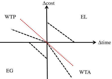
Sign effects are an example of the more general concept reference dependence. Based on the assumption that a reference-free VTTS exists, De Borger & Fosgerau (2008) propose a way to remove reference-dependence, thereby obtaining the reference-free VTTS. The idea is to introduce a value function superimposed on an underlying utility function, where only the value function takes the reference point into account, while the underlying utility function is reference-free. By estimating both the parameters of the value function and the utility function, the superimposed value function can be removed, and with it the reference dependence. De Borger and Fosgerau show that their theory is consistent with a series of econometric tests. In particular, the theory predicts a certain, testable relation between the indifference curves in four “quadrants”, which is best explained graphically (Figure 2).

8

Figure 2. Four types of binary choices relative to a reference point, with different indifference curves in different quadrants.

The origin of coordinates in

Figure 2 corresponds to the reference trip. The four quadrants relate to different types of binary choices: “willingness to pay” (WTP) choices compare the reference trip to a faster but more expensive alternative; “willingness to accept” (WTA) choices compare the reference to a cheaper but slower alternative; “equivalent gain” (EG) choices compare a cheaper to a faster alternative (relative to the reference); “equivalent loss” (EL) choices compare a more expensive to a slower alternative (relative to the reference). As shown in the figure, loss aversion implies that the indifference curve through zero (dashed) have a kink in the reference point (Bateman, Munro, Rhodes, Starmer, & Sugden, 1997). To uncover the reference-free indifference curve (dotted), the kink has to be removed. A central result from De Borger and Fosgerau is that the underlying reference-free value of time _,- can be obtained as a geometrical average of the different type choices:

,-= ( ./0∗ ./1)½= ( 34∗ 35)½ (6)

∆

cost

∆

time

WTP

WTA

EL

EG

∆

cost

∆

time

WTP

WTA

EL

EG

9

where _./0, _./1, ₃₄ and ₃₅ are the slopes of the indifference curves in the respective four quadrants. This equality offers a way to test the theory empirically by testing the equality between the two geometric averages.

In practical estimation, this means that a dummy parameter is introduced in (see (5)) for each quadrant but one. Formula (6) predicts the following relation between the dummy parameters: ½(EG+EL) = ½(WTP) (the WTA dummy is normalized to zero). Estimation results are shown in Table 2. The correspondence for public transport is remarkably good. For car trips, the geometric means differ somewhat, but the difference is not statistically significant. Interestingly, the deviation from the DeBorger-Fosgerau formula can be explained. The car data consists of two separate surveys, which are different in one respect: in the first survey (from 2006), the “reference alternative” in the choice experiment is perturbed slightly with respect to the actual reference trip6_{, while the second part (from 2007) used the exact reference trip. The}

deviation from the predicted relation (6) turns out to stem from the perturbed reference in the 2006 data: when only the non-perturbed-reference data from 2007 is used, the formula holds almost exactly (the difference has a t-statistic of 0.65).

4.2

Size effects

The second type of “experimental artefact” that needs to be controlled for is size effects. For binary choice experiments, size effects will often cause the value of time to be higher the larger the time difference is between the two alternatives. Even if this effect is “real” in the sense that it is not just an artefact of the hypothetical setting, it is not relevant for appraisal purposes: the VTTS cannot depend on the size of time (or cost) savings, since these are only defined in experimental and other short-run settings. Analysing the Norwegian VTTS data, Hjorth & Fosgerau (2011) find that the size effect can also be explained by reference-dependence. However, in this case it is not possible just to take out the effect.

One of the advantages of MRS-space estimation is the ease of which size effects can be controlled for: the differences in time and cost between the binary alternatives (∆t and

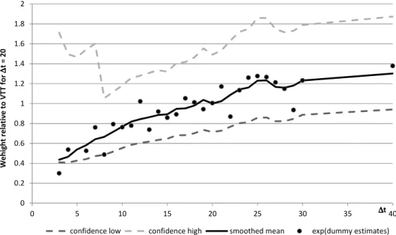
∆c) can be introduced as covariates in the estimation. In this study, ∆t is significant for car and long distance public transport while ∆c is not significant for any of the modes. Figures 4 and 5 demonstrate how the VTTS depends on ∆t. They are obtained through semi-parametric estimation: a dummy parameter is estimated for each value of ∆t, in addition to the other covariates7_{. The dummy for} ∆_{t=20 min is normalized to zero, such}

that the VTTS for ∆t=20 min has weight 1. For car, the VTTS at ∆t=5 is about 0.7 times the VTTS for ∆t=20 min. For long distance public transport, the VTTS at ∆t=5 is about 0.5 times the VTTS for ∆t=20 min. The dashed lines show 95% confidence intervals.

6

This was because the 2006 survey was intentionally an exact repetition of the 1995 value-of-time survey, so the results could be compared. The original reason for perturbing the reference alternative was to try to reduce reference-dependence phenomena.

7_{The effect of} ∆_{t in this data have also been examined using a pure non-parametric estimation, see}

Börjesson et al. (2010). The semi-parametric estimation shown here controls for the effect of other design variables, such as travel distance of the reference trip, which non-parametric estimation cannot do. It is important to control for other design variables, since ∆t is correlated with these that also have an impact on the VTTS. In particular, the VTTS is generally found to increase with observed travel distance which is strongly correlated with ∆t in the SC experiment by design.

10

Figure 3 Non-parametric estimates of the influence of ∆t on VTTS, car trips.

Figure 4: Non-parametric estimates of the influence of ∆t on VTTS, long-distance public transport.

The VTTS is significantly different from zero even for small ∆t. In other words, there is no visible “inertia” or “threshold” effect: even the first minute of a travel time saving has some value. The effect of ∆t was also explored by piecewise linear estimation showing that the VTTS increases with ∆t up to about 45 minutes for car and up to 25 minutes for long distance public transport. For regional public transport, the effect of

∆t is not significant.

Many authors have discussed the source the ∆t effect, and how to deal with it in appraisal (e.g. Mackie et al. 2001; Fowkes 1999; Hultkrantz, 2001; Fosgerau, 2006; Bates and Whelan, 2001). Different, partly overlapping interpretations can be

0.2 0.4 0.6 0.8 1 1.2 1.4 1.6 0 5 10 15 20 25 30 35 40 W e h ig h t re la ti v e t o V T T f o r ∆∆∆∆ t = 2 0 ∆∆∆∆t

confidence low confidence high smoothed mean exp(dummy estimate)

0 0.2 0.4 0.6 0.8 1 1.2 1.4 1.6 1.8 2 0 5 10 15 20 25 30 35 40 W e h ig h t re la ti v e t o V T T f o r ∆∆∆∆ t = 2 0 ∆∆∆∆t

11

conjectured. First, it is possible that individuals actually value small time gains less per minutes than large ones, because small time savings cannot easily be used for any meaningful activities in the short run when schedules are already settled. Since time cannot be saved for future use, unlike money, this would decrease the VTTS. Second, the size effect could arise because respondents simplify the choice process by disregarding small differences between alternatives. Generally speaking, individuals often make increasingly rational choices when differences are larger and stakes are higher (Smith and Walker, 1993; Levitt and List, 2007). In the present context, this means that respondents become increasingly rational and careful in their choices when the time savings increases. This would imply that the size effect does not arise because passengers actually value small time savings less per minute than large ones, but because of a “simplification error” in how they answer the stated choice questions. Third, if travel times are unreliable, it is possible that respondents do not consider travel time savings that lie within the normal variation of the travel time.

To arrive at a result that can be recommended for use in appraisal, we need to choose a

∆t at which to evaluate the expression for the VTTS. Although slightly different, all these interpretations land in a conclusion that the relevant, reference-free VTTS will tend to be underestimated at small ∆t:s. We have chosen to evaluate the VTTS at ∆t = 20 minutes for long trips (longer than 100 km) and at ∆t = 15 minutes for short trips (shorter than 100 km)8_{. The primary reason for these choices is that we wish to avoid}

evaluating at small ∆t:s, for the reasons explained above.

Understanding the influence of attribute differences on stated choice valuations may be the outstanding unresolved issue in this research field. Our results enable a better understanding of how ∆t affects the VTTS – but we can still only conjecture why. Even if there is no certainty or consensus about how size effects should be interpreted or handled, we want to emphasize that it is often extremely important to control for them. If not, the experimenter runs the risk of getting results that depend crucially on the SP design – the larger the time differences are the higher the estimated valuations are likely to become! We are aware of several examples where this has produced strange and counter-intuitive results. One example is the Swedish 1995 VTTS study, where the SP design for drivers turned out to have very small time differences in the design due to a large share of short trips. This led to a very low VTTS for car drivers, which was then incorporated into Swedish appraisal guidelines for many years.

5

EFFECTS OF TRIP AND TRAVELLER CHARACTERISTICS

The theory of the value of travel time is well developed. Becker (1965) seems to be the first to propose a general theory for the allocation of time and income. His framework was later refined by DeSerpa (1971) and Evans (1972). Jara-Díaz (2003) and Jara-Diaz & Guevara (2003) extend the classic framework into a general time allocation and consumption framework.

In short, the monetary valuation of a travel time saving depends on three factors: the opportunity value of time (the utility that could be attained if the travel time was used for some other activity, also called the “resource value”), the direct utility of travel time (compared to some reference activity), and the marginal utility of money:

8

12

67" 8 #9 :768" ;<8 =#==#: >; 67" 8 #9 ;<8 − ?;:8 ;"; #9 :768" ;<8 <7:$;>7" ;"; #9 <#>8

If a travel time saving can be converted into paid work (by working more hours) or a wage increase (by choosing a better paid work further away from home), the first part is equal to the after-tax wage rate, and the value of time becomes

67" 8 #9 :768" ;<8 = @7$8 :7 8 − ?;:8 ;"; #9 :768" ;<8 <7:$;>7" ;"; #9 <#>8

These marginal utilities cannot be observed directly, but we may expect that they are affected by various observable characteristics of the trip and the traveller. The direct utility of travel time should be affected by factors such as the comfort of the mode and the productivity or enjoyability of the trip. Further, it is measured in comparison to the utility of being at the origin or the destination9_{, and hence it will be lower (and the}

value of time higher) on the way to an important meeting or on the way home late at night (hence the comparatively high share of taxi trips late at Saturday nights). The resource value of time should increase the less available time the traveller has in general. Hence, we may expect it to be higher for employed people and for parents of small children. The marginal utility of money should be related to the income of the traveller and his or her medium-term fixed costs (which in turn may depend on factors such as the number of family dependants).

5.1

Estimation results

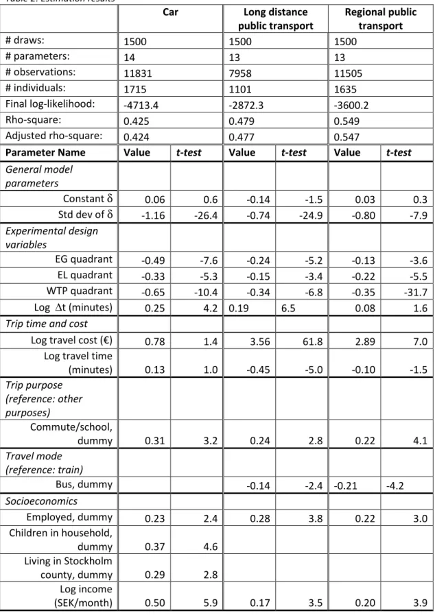
From the discussion above, it follows that the VTTS can be expected to vary both with characteristics of the trip and the traveller. As shown in the previous section, it also varies with characteristics of the choice experiment. Complete estimation results are shown in Table 2. Note that the parameters are easily interpreted: a value of β for a dummy variable means that the value of time increases with a factor exp(β).

9 _{If the departure time is optimally chosen, the marginal utilities of being at the origin and the} destination are equal (Vickrey, 1973; Tseng & Verhoef, 2008).

13

Table 2: Estimation results

Car Long distance

public transport Regional public transport # draws: 1500 1500 1500 # parameters: 14 13 13 # observations: _{11831 7958 11505} # individuals: _{1715 1101 1635} Final log-likelihood: -4713.4 -2872.3 -3600.2 Rho-square: 0.425 0.479 0.549 Adjusted rho-square: _{0.424 0.477 0.547}

Parameter Name Value t-test Value t-test Value t-test

General model parameters Constant δ 0.06 0.6 -0.14 -1.5 0.03 0.3 Std dev of δ -1.16 -26.4 -0.74 -24.9 -0.80 -7.9 Experimental design variables EG quadrant -0.49 -7.6 -0.24 -5.2 -0.13 -3.6 EL quadrant -0.33 -5.3 -0.15 -3.4 -0.22 -5.5 WTP quadrant -0.65 -10.4 -0.34 -6.8 -0.35 -31.7 Log ∆t (minutes) 0.25 4.2 0.19 6.5 0.08 1.6

Trip time and cost

Log travel cost (€) 0.78 1.4 3.56 61.8 2.89 7.0

Log travel time

(minutes) 0.13 1.0 -0.45 -5.0 -0.10 -1.5 Trip purpose (reference: other purposes) Commute/school, dummy 0.31 3.2 0.24 2.8 0.22 4.1 Travel mode (reference: train) Bus, dummy -0.14 -2.4 -0.21 -4.2 Socioeconomics Employed, dummy 0.23 2.4 0.28 3.8 0.22 3.0 Children in household, dummy 0.37 4.6 Living in Stockholm county, dummy 0.29 2.8 Log income (SEK/month) 0.50 5.9 0.17 3.5 0.20 3.9

Table 2 shows that bus trips have a lower value of time than train trips, when trip and traveller characteristics are controlled for. Other differences between modes are not directly revealed by inspection of Table 2. However, pooling all modes in one model

14

shows that, ceteris paribus, the VTTS is highest for car trips, followed by long-distance train, regional train and finally bus trips.

The VTTS depends on the time and the cost of the trip. For drivers, travel time and travel cost are not significantly different from zero (although they are jointly significant, meaning that if one of them is taken out, the other variable is significant). For public transport, the cost variable is highly significant. The effect of travel time and travel cost on the VTTS may be due to a number of factors affecting the VTTS in different directions, e.g. self-selection effects, comfort effects and decreasing marginal utilities of time and money.

The purpose of the trip affects the value of time to some extent. Commuting/school trips have around 30% higher VTTS than other private trips (school trips with car have a VTTS more similar to the VTTS for “other” trips, and are thus included in the latter segment). Note that income and employment status are already controlled for, so it is in fact the trip purpose as such that affects the VTTS. There are several possible explanations for this: time savings for work trips may be easier to convert into money by working more hours; time may be scarcer during working days (affecting the resource value of time); there may be more binding scheduling constraints connected to work trips.

A large number of socioeconomic variables were tested, but only four were significant: employment status, income, whether there are children in the household and whether the respondent lives in the county of Stockholm. The two latter were only significant for drivers. The VTTS is, all else equal, higher for employed and those having children in the household. This is consistent with the expectation that the resource value increases the less available time one has (note that income differences are controlled for separately). There is no significant gender effect. The finding that the VTTS increases with income is consistent with the expectation that the marginal utility of money decreases with income.

The most intriguing effect is that the VTTS for car trips is considerably higher in the county of Stockholm than in the rest of the country (a factor 1.3). There is no corresponding effect for the second and third largest cities in Sweden (Gothenburg and Malmö). There are several possible explanations:

- Road congestion is considerably higher in Stockholm than elsewhere, which would increase travel time variability, and also decrease the direct utility of travel time through a “comfort” effect (Wardman & Nicolás Ibáñez, 2012). Since the choice experiments did not explicitly control for these factors, the value of time may be increased by these phenomena.

- Self-selection will cause trips with high values of time to choose fast and expensive modes, which in the case of regional trips (which constitutes the bulk of the trips in the sample) means choosing car over public transport, cycling or walking. Theoretically, there will be a “split point” in the value of time distribution, over which travellers will choose car and below which they will choose other modes. The better the public transport supply is, the higher this split point will be, the lower the car mode share will be, and the higher the value of time of car travellers will be. In Stockholm, the public transport supply is much better than elsewhere in Sweden, and consequently the car share is considerably lower. We would expect that this should translate into a higher value of time for car drivers: loosely speaking, only trips with values of time in the high end of the value of time distribution will choose car in Stockholm.

15

- Stockholm inhabitants have longer total travel times, giving them less residual time for activities, and hence the resource value of time should be higher. It is interesting to note that the finding that Stockholm inhabitants have a higher value of time is consistent with previous findings that citizens of larger cities walk faster in many different cultural settings (Milgram, 1970; Bornstein and Bornstein; 1976). It should be pointed out that even after controlling for the factors in the estimation above there is still a large variation in the VTTS: the standard deviation of δ is highly significant for all modes. Hence, even seemingly identical travellers on seemingly identical trips may have very different values of time.

6

VALUES OF TIME FOR USE IN APPLIED APPRAISAL

As shown in the preceding section, the VTTS differs along several dimensions. But in applied appraisal, it is usually only possible to take into account differences in trip purpose, trip length, travel mode and region. Regarding socioeconomic differences (children, employment status etc.), few transport models are built to handle such details. Instead, these variables will be partly captured through their correlation with mode, trip purpose and trip length. Trip length is essentially a proxy for travel cost and travel time, but it is practical to let the value of time depend on trip length in applied appraisal, since both travel cost and travel time change over time and also as a result of the policy measure or investment under study. For practical purposes, Swedish appraisal practice only takes trip length into account by separating “short” and “long” trips, where “short” trips are defined as “shorter than 100 km”. Most countries apply similar simplifications.

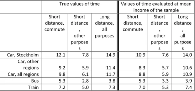
Table 3 shows values of time intended for use in applied transport appraisal. The values are differentiated with respect to mode, trip purpose, trip length and region. They are simulated by averaging the VTTS:s of all individuals in the estimation sample, weighted with travel distance. The table also shows VTTS controlled for income differences, i.e. the VTTS evaluated at the mean income of the sample.

The most contentious differentiation is that between Stockholm and the rest of the country. In the previous section we suggested some explanations of the fact that Stockholm car drivers have a higher value of time than car drivers elsewhere, even controlling for socioeconomic differences, trip lengths etc. Since all the possible explanations are consistent with the economic theory underlying standard appraisal, we see no reason not to differentiate the VTTS across regions, although we appreciate the political difficulties of implementing such a differentiation. As far as we know, no countries differentiate appraisal VTTS with respect to region. This seems to be partly because of the political difficulty to implement such differences, and partly because of an impression that differences in values of time depend mostly on income differences. Our results, however, show a higher value of time in Stockholm even after controlling for differences in income, employment status etc.

The differences across modes and trip distances in Table 3 are due partly to trip characteristics, such as trip purpose or the comfort of the mode, and partly to self-selection among travellers, i.e. travellers with high opportunity cost of time will tend to choose faster but more expensive modes. Fosgerau et al. (2010) find that the mode differences in values of time are due to both self-selection and comfort effects in the Danish VTTS study. Some of the heterogeneity in the opportunity cost of time can be explained by socioeconomic differences, such as differences in income or household

16

composition, but a substantial part is due to idiosyncratic variation between trips. Socioeconomic differences are far from the only source of VTTS differences between modes: even when controlling for all socioeconomic differences, car drivers have higher VTTS than train passengers which in turn have higher VTTS than bus passengers. In particular, income differences are not the main source of VTTS variation across modes or distances, which are further discussed below.

Table 3: Values of time for use in applied appraisal (€/hour). Actual values (left) and controlled for differences in income (right).

True values of time Values of time evaluated at mean income of the sample Short distance, commute Short distance , other purpose s Long distance, all purposes Short distance, commute Short distance , other purpose s Long distance , all purpose s Car, Stockholm 12.1 7.8 14.9 10.9 7.6 14.0 Car, other regions 9.2 5.9 11.4 8.3 5.7 10.6

Car, all regions 9.8 6.1 11.7 8.8 5.9 10.9

Bus 5.3 2.8 3.8 5.3 3.3 3.9

Train 7.2 5.0 7.3 7.0 5.3 7.4

For investment appraisal the residual idiosyncratic variation in VTTS, captured by δ, does not matter for the outcome of a cost-benefit analysis: it is enough to know the average VTTS. A substantial intra-individual variation would, however, have a direct impact on equity analysis. Moreover, for appraisal of other types of changes – notably all sorts of pricing schemes – the idiosyncratic variation in the value of time may have profound implications for the outcome of a cost-benefit analysis (see for instance Verhoef and Small (2004)). Since our material is based on just one observation per individual, we cannot say anything about the magnitude of intra-individual variation compared to inter-individual variation.

There has been a long debate in the literature regarding whether values of time in applied appraisal should be allowed to vary with income. Some authors have argued that appraisal should be based on actual willingnesses-to-pay (see Sugden (1999) in the context of transport policy and appraisal, and Harberger (1978) and Harberger (1980) in the context of general cost-benefit analysis). Others have argued that this implicitly assumes welfare weights inversely proportional to the marginal utility of income, hence giving more weight to high-income groups than to low-income groups (Pearce & Nash, 1981; Galvez & Jara-Diaz, 1998; Mackie, Jara-Díaz, & Fowkes, 2001). The position of the latter group of authors can be summarized as follows: Assume that the decision problem is to create maximal total utility assuming equal welfare weights (i.e. a strictly utilitarian welfare function) in a context where travellers are the final beneficiaries of transport improvements, individuals differ in terms of marginal utility (MU) of travel time and MU of money, and acquiring public funds is associated with some welfare loss (e.g. due to deadweight losses)10_{. Then, it can be shown that travel}

10 _{This provides an explanation of why there may be differences in MUs of money across individuals,} even if the government is “almighty and benevolent” and uses unit welfare weights.

17

time improvements should be converted to money using a “value of time” which is the ratio between the travellers’ MU of time and the paying group’s average MU of money – which is not necessarily the same as the travellers’. This means that the relevant VTTS will depend on how the policy is funded. If the funding of a project comes from the travellers themselves, for example in the form of ticket revenues or road user charges, then the welfare measure should be based on the VTTS of the travellers. If the policy is publicly funded, then the VTTS should be based on the MU of money of the relevant funding source, for example a state, region or city; the VTTS will be different for regionally financed projects compared to nationally funded projects. Note that differences in the MU of time should not be discarded. Further, note that the conclusion that income effects should be removed is obtained starting from a strictly utilitarian welfare function. It should not be confused with the type of “weighted CBA” where explicit distributional weights are introduced in the welfare function to capture equity concerns.

A common counter-argument is the Kaldor-Hicks argument: as long as the winners can compensate the losers, the government is free to carry out redistributions by a number of policy instruments, including taxes and various welfare systems. This argument is open to a number of objections, however, since governmental redistributions in reality are constrained in a number of ways, by political constraints and the deadweight cost of taxation to name but two.

A more persuasive counterargument is that the argument for removing income effects from the VTTS assumes that travellers are the final beneficiaries of transport improvements. But in the long run, the benefits will be dispersed across the economy, and the final beneficiaries will be a mixture of land owners, tax payers, transport companies, employers, businesses, customers and travellers. Assuming perfect markets, benefits will be captured by land owners, but in a reality with imperfect competition, price restrictions and planning regulations, the final incidence is virtually impossible to know. This would be an argument to use actual values of time, since it is benefits in terms of actual willingnesses-to-pay that are dispersed across the economy. The crux of the debate seems to be what should be assumed about the final beneficiaries of a transport investment. In a situation where one has reason to believe that a substantial part of the benefits stay with the travellers, differences in VTTS due to income differences should be removed and the right part of Table 3 should be used; otherwise, the actual VTTS (the left part of Table 3) should be used. After lengthy discussions, the new Swedish Appraisal Guidelines recommends the valuations from the left part of Table 3, i.e. without removing income effects.

Earlier value of time research has run into problems when trying to isolate the effect of income differences, since it correlates with several other characteristics. Estimating in MU space makes it much more difficult to introduce many covariates simultaneously. Estimating in MRS space, however, enables the analyst to identify and remove the effect of income differences on the VTTS more precisely. In this sense, the present study can be viewed as finally making possible the suggestion of Galvez & Jara-Diaz (1998) and Mackie et al. (2001): that income effects should be removed from the appraisal VTTS without removing differences in MUs of travel time.

As shown in Table 3, controlling for income differences changes the VTTS only slightly in most cases. Most of the differences across modes, purposes and trip lengths remain, showing that these differences are mainly driven by comfort factors and self-selection due to other variables than income differences. Some values do change appreciably, though: the value for short commuting train trips decreases by 40%, and the value for

18

short other-purpose bus trips increases by 30%. The other differences are not small primarily because the income elasticity on the VTTS is negligible, but because the differences in average income across modes, purposes and trip lengths are relatively small, see Table 1. Although there certainly are such differences, the main message of the table is that differences due to other factors (self-selection, comfort, type of trip etc.) are much larger.

It should immediately be pointed out that these are Swedish results. Sweden is a relatively affluent country, where most people can afford to own and use car (at least occasionally), and income differences are not very large (especially after tax). Still, income is a strong predictor of travel behaviour, both in terms of car ownership, car use, trip length and long-distance trip frequency, and there is a strong correlation between income and these variables in our sample as well. In all these respects, Sweden is similar to most other rich countries. Hence, we would expect that our conclusions would be typical for other rich countries, at least those with a relatively high public transport share.

The argument that income effects should be removed from the VTTS has lead several countries to adopt appraisal practices where all or almost all differences in the VTTS are removed, sometimes called “equity values” of time. This is clearly a misunderstanding of the debate (which is also specifically pointed out by Galvez & Jara-Diaz (1998)). This practice reduces the information contained in the appraisal, and eventually leads to the misallocation of resources across the transport sector. Differentiating the value of time in appraisal shows which kinds of travel time reductions will create most value to society. It can also lead to paradoxical results, where user-paid transport improvements can be judged to be socially unprofitable even if users would gladly pay for the improvement (Sugden, 1999).

Regarding general equity concerns – a wider issue than just income differences – it should be stressed that most people make many kinds of trips, with different modes, purposes and trip lengths. The difference in resource spending caused by differentiating the value of time in appraisal is hence not so much a difference across individuals than it is a difference across trips made by the same individual. Clearly, it can be perfectly logical that an individual values a travel time saving during his morning car commute than during his Saturday bus trip to a museum. Using only a single value of time for appraisal will destroy this distinction, and hence misallocate resources out of (in this case) misguided “equity concerns” – in this case, “equity concerns” would mean that the morning car commute “should” be valued exactly as the Saturday museum trip, despite that the individual would prioritize differently.

7

CONCLUSIONS

In this paper, we have given a synthesis of the results and insights from the Swedish value of time study. Recent econometric advances have made it possible to identify the value of time distribution and its dependence on different types of covariates more precisely. Our main conclusions can be summarized as follows:

- The value of time exhibits great variation, both because of observable characteristics of the trip and the traveller, and because of idiosyncratic variation.

19

- The value of time varies both with traveller characteristics (income, having children, employment, living in Stockholm) and with trip characteristics (travel mode, travel time, travel cost and travel purpose).

- The value of time distributions seems to be close to a truncated normal distribution in the Swedish, Danish and Norwegian value of time data.

- Although the income effect on the value of time is considerable, it is far from the main source of the observed differences in value of time across modes, trip purposes, trip lengths etc. Removing the income effect from the value of time changes the values in segments relevant for appraisal only slightly.

- Whether income effects should be removed from the value of time in appraisal depends on which groups pay for the suggested policy and on the final incidence of benefits.

- Even if one wishes to remove income effects from the value of time, adopting a single, or few, values of time in appraisal practice because of income equity concerns is an overreaction. This practice removes heterogeneities in the valuations that are highly relevant for appraisal, if the purpose is to find policy measures and investments that maximize aggregate utility.

- When estimating a valuation distribution, data must support a sufficient range of the distribution. Solely using parametric estimation may hide whether this is in fact the case; in worst case, conclusions are drawn based on behaviour of the tail of a distribution that is not supported by the data.

- Estimating in MRS space seems to be more consistent with both the Swedish and Danish value of time data. It also makes it easier to introduce covariates in the estimation, compared to the standard MU space estimation.

- Size and sign effects need to be controlled for. If not, results will depend on the characteristics of the experiment, such as the design of the choice experiment. - Sign effects (loss aversion) can be controlled for and removed to reveal the

”reference-free” value of time.

- Size effects are not only present for ”small” time savings, but in most cases over the entire range of time differences. The interpretation of the size effect, and how they should be handled, may be the outstanding unresolved issues in stated choice valuation.

The main results of the paper are values of time for use in applied appraisal. These are segmented with respect to mode, trip purpose, trip distance and residential region. Further segmentation is possible but usually not feasible in practice. Both values with and without income effects present have been presented.

20

8

REFERENCES

Bateman, I., Munro, A., Rhodes, B., Starmer, C., & Sugden, R. (1997). A Test of the Theory of Reference-Dependent Preferences. The Quarterly Journal of Economics, 112(2), 479-505.

Becker, G. S. (1965). A Theory of the Allocation of Time. The Economic Journal, 75(299), 493-517.

Bierlaire, M. (2003). BIOGEME: A free package for the estimation of discrete choice models. Proceedings of the 3rd Swiss Transportation Research Conference, Ascona, Switzerland.

Bierlaire, M. (2008). An introduction to BIOGEME Version 1.6, biogeme.epfl.ch.

Börjesson, M. (2010a). Inter-temporal variation in the marginal utility of travel time and travel cost. Presented at the World Conference of Transport Research. Börjesson, M. (2010b). Valuating perceived insecurity associated with use of and access

to public transport. Proceeding from the European Transport Conference, Glasgow.

Börjesson, M., Fosgerau, M., & Algers, S. (2012a). Catching the tail: Empirical identification of the distribution of the value of travel time. Transportation Research A, 46(2), 378-391.

Börjesson, M., Fosgerau, M., & Algers, S. (2012b). On the income elasticity of the value of travel time. Transportation Research A, 46(2), 368-377.

Daly, A., Tsang, F. & Rohr, C. (2011). The value of small time savings for non-business travel Proceeding from the European Transport Conference, Glasgow.

De Borger, B., & Fosgerau, M. (2008). The trade-off between money and travel time: A test of the theory of reference-dependent preferences. Journal of Urban Economics, 64(1), 101-115.

DeSerpa, A. C. (1971). A Theory of the Economics of Time. The Economic Journal, 81(324), 828-846.

Dillén, J., & Algers, S. (1998). Further research on the national Swedish value of time study. Selected Proceedings of the 8th World Conference on Transport Research, 3, 135–148.

Evans, A. W. (1972). On the theory of the valuation and allocation and time. Scottish Journal of Political Economy, 19(1), 1-17.

Fosgerau, M. (2006). Investigating the distribution of the value of travel time savings. Transportation Research B, 40(8), 688-707.

Fosgerau, M. (2007). Using nonparametrics to specify a model to measure the value of travel time. Transportation Research A, 41(9), 842-856.

Fosgerau, M., & Bierlaire, M. (2007). A practical test for the choice of mixing distribution in discrete choice models. Transportation Research Part B, 41(7), 784-794.

Fosgerau, M., Hjorth, K., & Lyk-Jensen, S. V. (2010). Between-mode-differences in the value of travel time: Self-selection or strategic behaviour? Transportation Research D, 15(7), 370-381.

Galvez, T. E., & Jara-Diaz, S. R. (1998). On the social valuation of travel time savings. International Journal of Transport Economics, 25(1), 205-219.

Harberger, A. C. (1978). On the Use of Distributional Weights in Social Cost-Benefit Analysis. The Journal of Political Economy, 86(2), S87-S120.

Harberger, A. C. (1980). On the Use of Distributional Weights in Social Cost-Benefit Analysis: Reply to Layard and Squire. The Journal of Political Economy, 88(5), 1050-1052.

Hjorth, K., & Fosgerau, M. (2011). Loss Aversion and Individual Characteristics. Environmental and Resource Economics, 49(4), 573-596.

Jara-Díaz, S. R. (2003). On the goods-activities technical relations in the time allocation theory. Transportation, 30(3), 245-260.

21

Jara-Diaz, S. R., & Guevara, S. R. (2003). Behind the Subjective Value of Travel Time Savings. Journal of Transport Economics and Policy, 37, 29-46.

Mackie, P. J., Jara-Díaz, S., & Fowkes, A. S. (2001). The value of travel time savings in evaluation. Transportation Research Part E, 37(2-3), 91-106.

Milgram, S. (1970). The Experience of Living in Cities. Science, 167(3924), 1461 -1468. Pearce, D. W., & Nash, C. A. (1981). The Social Appraisal of Projects – A Text in

Cost-Benefit Analysis. London: Macmillan.

Ramjerdi, F., Flügel, S., Samstad, H., & Killi, M. (2010). Value of time, safety and environment in passenger transport ? Time - Transportøkonomisk institutt. Retrieved from http://www.toi.no/article29726-29.html

Sugden, R. (1999). Developing a consistent cost-benefit framework for multi-modal transport appraisal (Report to the Department for Transport). University of East Anglia.

Tseng, Y.-Y., & Verhoef, E. T. (2008). Value of time by time of day: A stated-preference study. Transportation Research B, 42(7-8), 607-618.

Wardman, M., & Nicolás Ibáñez, J. (2012). The congestion multiplier: Variations in motorists’ valuations of travel time with traffic conditions. Transportation Research A, In Press.

Verhoef E.T., & Small K.A. (2004). Product Differentiation on Roads. Journal of Transport Economics and Policy, 38(1), 127-156.

Vickrey, W. (1973). Pricing, metering, and efficiently using urban transportation facilities. Highway Research Record, 476, 36-48.