Towards Autonomic Software Product Lines (ASPL) - A Technical Report

Department of Computer Science

Linnaeus University

Technical Reports

351 95 V¨axj ¨o Sweden http://lnu.se

Towards Autonomic Software Product Lines (ASPL)

-A Technical Report

Nadeem Abbas

nadeem.abbas@lnu.se

Jesper Andersson

jesper.andersson@lnu.se

Welf L ¨owe

welf.lowe@lnu.se

LNU-CS-AdaptWise-TR-2011NA01

This report describes a work in progress to develop Autonomic Software Product Lines (ASPL). The ASPL is a dynamic software product line approach with a novel variability handling mechanism that enables traditional software product lines to adapt themselves at runtime in response to changes in their context, requirements and business goals. The ASPL variability mechanism is composed of three key activities: 1) profiling, 2) context-aware composition, and 3) online learning. Context-profiling is an offline activity that prepares a knowledge base for context-aware composition. The context-aware composition uses the knowledge base to derive a new product or adapts an existing product based on a product line’s context attributes and goals. The online learning optimizes the knowledge base to remove errors and suboptimal information and to incorporate new knowledge. The three activities together form a simple yet powerful variability handling mechanism that learns and adapts a system at runtime in response to changes in system context and goals. We evaluated the ASPL variability mechanism on three small-scale software product lines and got promising results. The ASPL approach is, however, is yet at an initial stage and require improved development support with more rigorous evaluation.

1

Introduction

Improving system quality, time-to-market, and development cost are common business goals for the software industry [21]. To achieve these goals, a well-defined development strategy that results in improved productivity and efficiency is needed. Software systems in a same category or application domain, for instance, healthcare, accounting, and payroll systems, have commonalities in their features, structure, and behavior. These commonalities open a window of opportunity for development with reuse. The software developers exploit this opportunity by adopting product lines engineering strategy [48, 64].

A software product line (SPL) is “a set of software-intensive systems sharing a common, managed set of features that satisfy the specific needs of a particular market segment or mission and that are developed from a common set of core assets in a prescribed way” [47]. The basic philosophy behind product line engineering is to define a high-level reference architecture also known as product line architecture, and a platform of reusable artifacts. The product line architecture and the reusable artifacts are defined with variation points and variants that can be (re)configured to derive products in a product line. The products are derived by specializing the product line architecture according to products’ needs selecting component variants from the platform and binding them to variation points. Most software products instantiated from traditional SPLs bind variants statically or at the latest at load time. Such products perform well in a setting where changes to requirements, product environment, or other related concerns are rare. However, in a dynamic world characterized by more frequent changes, the traditional SPLs fail to adapt themselves in response to changes in their requirements, contexts or environments, and business goals [4].

The need to address runtime variations in product lines’ requirements, environments and business goals call for extensions to the traditional software product line engineering approaches. To that end, this report introduces an Autonomic Software Product Lines (ASPL) [2] engineering approach. The ASPL is a dynamic software product line approach[33] established on the basis of software product line engineering [50], autonomic computing [37] and context-aware computing [53]. The main contribution of the ASPL is a dynamic variability handling mechanism that

enables traditional software product lines to design and develop self-managing or self-adaptive software systems. A self-adaptive software system is capable of adapting its structure and behavior in response to changes in its requirements, business goals and the system itself [19].

The ASPL variability handling mechanism is composed of three principal activities: 1) context-profiling, 2) context-aware composition, and 3) online learning. Context-profiling is an offline training activity performed to prepare a knowledge base for the context-aware composition. The context-aware composition is a product or application engineering activity that uses the knowledge base to derive a product by selecting best-fit components and component variants.The knowledge base prepared by offline context-profiling may become obsolete or sub-optimal at runtime due to changes in the product line business goals, requirements, and environment. The online learning activity implements a runtime learning strategy to optimize the knowledge base.

To evaluate the ASPL approach, we conducted a set of experiments. The results indicate that the proposed approach results in a dynamic product line of self-adaptive software systems instrumented with mechanisms to support changes in context, goals and product line scope.

The remainder of this article is organized as follows. Section 2 introduces the concepts of product line engineering, autonomic computing, and software variability. These concepts form the background of the ASPL approach. The section 3 introduces the ASPL approach with a detailed description of the ASPL variability handling mechanism and underlying activities. The ASPL variability handling mechanism is evaluated in Section 4. In Section 5, we discuss related work. Section 6 concludes and discusses future work.

2

Background

The ASPL approach is found on the basis of software product line engineering and autonomic computing. The key contribution of the ASPL approach is a dynamic variability handling mechanism. Thus, before going into details of the ASPL approach, this section introduces product line engineering, autonomic computing, and software variability as a background of the ASPL approach.

Domain Engineeering Domain Analysis Domain Implementation Domain Verification & Validation

Product Engineeering

Product Requirements

Product Analysis & Design

Product Implementation

Product Verification &

Validation Product Line Management

Product Line Scoping

Product Line Evolution Management

Product Line Engineering

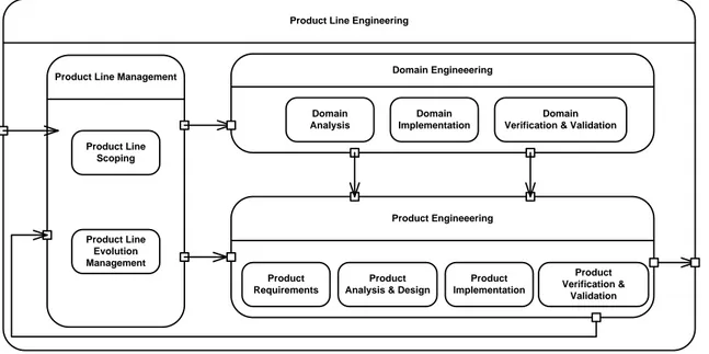
Figure 1: Product Line Engineering (PLE) activities

2.1

Product Line Engineering

Product Line Engineering (PLE) is a systematic reuse strategy that promotes domain specific, intra-organizational reuse based development with reduction in cost and improvement in quality [46]. It exploits commonalities among similar products while managing variability efficiently. It is built on top of a foundation of software architecture [7] and improves reuse by deploying tailored processes. An overview of PLE processes and process activities is depicted in Figure 1. A PLE framework typically involves three processes: 1) Product Line Management, 2) Domain Engineering, and 3) Product Engineering. An overview of these processes is given below.

Knowledge Monitor Execute Analyze Plan Sensor Effector Effector Managed Element Sensor

(a) Autonomic Element: MAPE-K Loop

Reflection Model Reflecive

Computation

1..* Reasons about and acts upon

Monitor Analyze Plan Execute

Reflective Subsystem 1..* 1..* Autonomic Element 0..* adapts Subsystem 0..* monitors

(b) FORMS primitives for an Autonomic Element

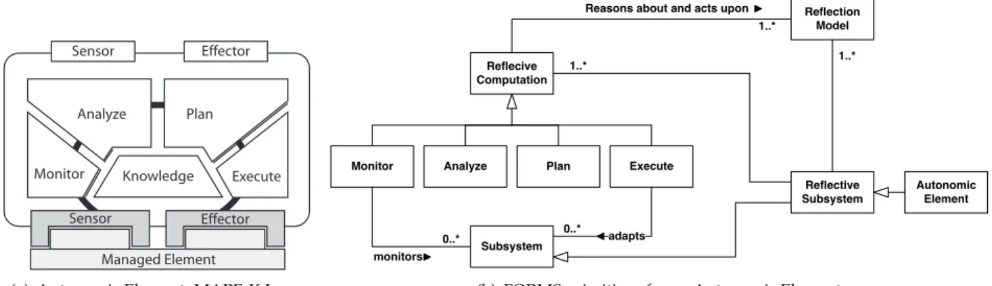
Figure 2: Basic structure of an Autonomic Element

Product Line Management (PLM) process is responsible for managing a product line’s scope and evolution. It uses data from two primary sources, 1) market and 2) product engineering projects, to control and manage evolution. Based on changes in a market, the PLM initiate domain engineering activities such as adding support for new market requirements. The PLM also monitors product engineering projects and uses the monitored data to control product line scope. For instance, in product engineering projects, product-specific requirements may result in product-specific variants and sometimes new features. Some of these variants may be candidates for inclusion in a product line. The PLM process decides on these matters and triggers domain engineering activities that refactor product-specific components for inclusion in a product line.

Domain Engineering process defines and realizes commonalities and variabilities of a product-line [50]. Its principal responsibility is to establish and maintain a set of application domain specific platform of reusable artifacts. Moreover, the domain engineering process provides support for product engineering activities, for instance, a lookup service to find reusable artifacts. The reusable artifacts produced as a result of the domain engineering range from domain requirements, design, and implementations to domain tests. These artifacts are designed to be flexible and customizable to support reuse across several products or applications in a domain. The flexibility of software artifacts and systems composed of these artifacts is known as software variability [50], see Section 2.3 for details about the software variability.

Product Engineering also known as application engineering produces individual software applications or products with reuse from the platform established by the domain engineering process [50]. The product engineering process is triggered by the PLM and is driven by product-specific requirements. As shown in the Figure 1, the product engineering process involves traditional software development process activities such as requirements engineering, analysis and design and implementation. However, it differs from traditional software processes in a way that it builds upon reusable artifacts offered by the domain engineering instead of developing them from scratch. The ultimate objective of the product engineering and all other product line engineering processes is to maximize the reuse as much as feasible.

2.2

Autonomic Computing

Autonomic computing (AC) is a computing model envisioned by IBM [37] to design and develop self-managing systems. A primary goal of the AC is to develop autonomic systems that are capable of adapting themselves independently with no or minimal external control and intervention. Managing large and complex inter-connected software systems manually through human administrators is a difficult, time consuming and error-prone task. Due to limited capabilities, human administrators are unable to adapt software systems in real time. Moreover, the uncertain human behavior causes uncertainties in manual system maintenance. The autonomic computing was proposed as a solution to deal with the complexity and difficulty of managing large and complex software systems.

An autonomic system is composed of several autonomic elements (AEs). Figure 2(a) depicts the basic structure of an AE. The AE implements a MAPE-K feedback loop [13] to monitor and manage one or more managed elements. The managed element may be hardware such as a printer, router, or software such as word processors, web browser. The AE itself may be a managed element monitored and managed by another AE, for instance, to design large and complex software systems.

The MAPE-K feedback loop is composed of five components: Monitor, Analyze, Plan, Execute, and Knowledge. These components together form a control flow to maintain specified properties of a system (managed element).

Brief introduction of the MAPE-K components is given below.

Monitor component enables an AE to observe one or more managed elements and their operating environments. It collects, aggregate, and report monitored data to the knowledge component.

Analyze component processes and analyzes data reported by the monitor component. The fundamental objective of the analysis is to determine whether the monitored managed element is satisfying its goals and requirements or not? If the managed element is not meeting the desired goals and needs, the analyze component calls plan component to prepare an adaptation plan.

Plan component prepares an adaptation plan on the basis of analysis results. The adaptation plan is an ordered set of actions that need to be performed on a managed element to ensure that the managed element fulfills its goals and requirements.

Execute component is responsible for performing adaptation actions on the managed element.

Knowledge component serves as a central knowledge base to share data and coordinate activities among monitor, analyze, plan and execute components. It stores data collected by the monitor, analysis reports prepared by analyze component and adaptation plans formed by the plan component. Moreover, it may contain additional data such as architectural models, goal models, policies, and change plans to support functions of the analysis and plan components [1].

The AE, in its structure and behavior, models a reflective system [5] that reflects adaptation actions on a managed system. To understand the AE architecture as a reflective system, we use primitives of FORMS, the FOrmal Reference Model for Self-adaptive systems [65]. Figure 2(b) depicts an AE in terms of the FORMS primitives. According to the FORMS primitives, an autonomic element is a specialization of a reflective subsystem. The reflective subsystem is an instance of a managed subsystem and is composed of two essential elements: reflective computation and reflection model. The reflective computation element monitors and adapts a managed subsystem with the help of monitor, analyze, plan, execute and reflection model (knowledge). The reflection model represents knowledge needed by reflective computation elements to analyze, reason about and plan actions to adapt the managed subsystem. This knowledge includes information about managed subsystem’s structure, environment, desired properties, goals, and objectives.

2.3

Software Variability

Software variability is the ability of a software system to be efficiently extended, customized or configured for (re)use in a specific context [61]. Variability of a software system or a product line is often modeled by defining variation points and variants in a system architecture. A variation point represents an open design decision that can be reconsidered. It models an insertion point where several variants of a system component can be bound and rebound. We distinguish two types of variation points: 1) open variation point and 2) closed variation point. An open variation point has no fixed variants associated with it, and new variants can be bound and rebound dynamically at runtime. Contrarily, a closed variation point is bound to a fixed variant at design or compile time, and the binding cannot be changed at runtime.

A variant is an alternatives realization of a feature. A feature is a distinct end-user visible characteristic of a system(s) [35], for instance, editing and formatting features of a word processor. In product line engineering, functional and quality requirements of a product line are often abstracted in terms of features [11]. Different products in a product line differ in their requirements of a feature; for instance, one product may require merge-sort algorithm based feature to sort the text, whereas other products may require bubble-sort or some other algorithm for the sorting feature. Such differences among products in a product line are referred as product line variability.

Product Line Architecture (PLA) plays a central role in product line engineering to define, model and manage a product line’s variability. To support reuse in a product line, the PLA is required to capture commonality and manage variability efficiently and effectively [41]. The PLA captures commonality by defining a set of core architectural components and handles variability by modeling a set of variation points and variants. Once the PLA is defined, it can be (re)used to derive several individual product architectures. To derive a product architecture, product designers are required to make design decisions for binding variants to variation points.

Figure 3 depicts a cause-effect diagram that illustrates a design decision for a variation point as a function of PLA, system goals, and system context. The system context here abstracts operating environments and inter-connected systems that affect the system behavior. The goals and context are decisive factors for design decisions where software designers or architects decides variants to be bound at a variation point.

Design Decision VP

Context Goals

Figure 3: Design decisions — causes and effect

Refined Design Decision VP

PLA

Goals Changed context

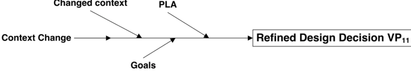
Figure 4: Reconsidering Design Decisions — Primary and Secondary Causes and Effects.

What is not illustrated in the Figure 3 is complex semantics where most decisions have dependencies to other decisions. For instance, the current context may impose restrictions on the variant set and the currently bound variant restricts what is reified as context. Such dependencies among factors controlling design decisions lead to challenges in decision making. Another problem is that neither the product line architecture nor the goals and context are fix-points. A product line evolves due to goal evolution, new variants are added, old ones are removed, products grow and context changes at runtime.

This calls software product lines to have new, more flexible and adaptable types of variability handling mecha-nisms that can adapt to and manage changes autonomously [4]. To that end, we introduce ASPL, a dynamic software product line engineering approach with a novel variability mechanism to manage variations at runtime. Autonomic computing, described below, provides foundations for the ASPL.

3

Towards Autonomic Software Product Lines

In Section 2.3, we described architectural design decisions as a cause-effect relationship where designers, based on their knowledge about context, goals, and product line architecture, decide which variants to bind to specific variation points. A factor we did not consider there is change, neither the product line architecture nor the goals and context are fixed points. A software product line evolves over time. New products and product variants with different features, goals and operating environments are introduced. Changes in a product line’s features, i.e., PLA, goals, and context may invalidate decisions made in product engineering. Consequently, the decisions made at product engineering or deployment time may have to be reconsidered at runtime to adapt the product line in response to the changes. In Figure 4, this is illustrated by a context change that invalidates a design decision for the variation point VP11. The context change triggers a reconsideration of the decision, the selected feature variants are

unbound, and new, better-suited variants are bound.

There exist few other non-trivial scenarios that require reconsideration of design decisions. One such scenario emerges when a self-optimizing web service application wants a change in its quality of service level. In a simple case, the quality model changes but not its input, i.e., the component properties contributing to the overall quality. In such cases, the optimization goal function is a black box that needs to be replaced. The old and the new optimization goal both conform to the same signature and are stateless functions. Hence, substitution is done smoothly using standard means.

In a more complex scenario, the relevant component properties may change as well, i.e., the new optimization goal is expressed on new properties of the component variants. For instance, memory consumption suddenly plays a role in the optimization where it has not even been monitored before. We still need to change the black box representing the optimization goal function. However, in this case, both the implementation and signature of the

optimization goal function may have changed. Additionally, a new infrastructure might have to be deployed to assess the new component properties. The exchange of the optimization goal is still possible but more advanced variability mechanisms, such as computational reflections [43], are needed to find the new signature of the quality goal function, derive a dynamic invocation based on new sensor results (which have to be installed dynamically and monitored as well), and invoke it.

An interesting observation from the above scenario is that the infrastructure that supports variability handling mechanisms must support the variability itself. For instance, it should support different variants of a goal function that may get bound and unbound according to changes in an optimization goal. Moreover, it should maintain different variants of the monitor, analyze, plan and execute functions to support a wide range of changes in systems’ context and goals. To manage variability in these and similar scenarios, we envision an Autonomic Software Product Lines (ASPL) approach. An overview of the ASPL approach is given below.

3.1

ASPL Overview

The ASPL is our vision to establish a dynamic software product line engineering approach that results in a product line of self-adaptive software systems. A self-managing or self-adaptive software system is capable of adapting itself in response to changes in its requirements, business goals, environment and the system itself [19]. Kephart et al. [37] enumerated four self-management properties as key characteristics of self-managing software systems: 1) self-configuration, 2) self-optimization, 3) self-healing and 4) self-protection. The ASPL currently targets only the first two self-management properties, self-configuration, and self-optimization. The self-configuration property requires that a software system is capable of reconfiguring itself either in response to a change or to assist in achieving some other system properties. The self-optimization property requires that a software system is capable of measuring and optimizing its performance.

Hallsteinsen et al. [33] specified a set of essential and optional properties of a dynamic SPL. A fundamental property of a dynamic SPL is a dynamic variability handling mechanism that enables a product line to deal with unexpected changes in functional or quality requirements and operating environment at runtime. The optional properties include context-awareness and automatic decision making. We envision the ASPL approach to provide traditional SPLs with a context-aware dynamic variability handling mechanism. The ASPL variability handling mechanism, described as follows, is a first step to realize the ASPL vision.

3.2

ASPL Variability Handling Mechanism

The ASPL variability handling mechanism enables traditional software product lines to adapt themselves at runtime in response to changes in their context, requirements and business goals. It is an extension of our profile-guided composition model [6] developed to improve the design and reuse of libraries of algorithms and data structures. The profile guided composition model forms a basic variability handling mechanism that composes a system by selecting best-fit component variants. The selection of best-fit variants is made based on a static knowledge base that is prepared offline (before runtime) by precomputing best component variants for certain call contexts. The static knowledge base suffers from variations at runtime and may lead to suboptimal compositions. To that end, the ASPL variability handling mechanism extends the profile guided composition model with an online learning activity that keeps the knowledge base updated.

The ASPL variability handling mechanism is composed of three core activities: 1) profiling, 2) context-aware composition, and 3) online learning. These activities are modeled and implemented as autonomic elements [37, 18]. The basic structure of an AE has been described in Section 2.2. The three activities together form a simple yet powerful mechanism to handle product line evolution and variations at runtime. Each of these activities is described as follows.

3.2.1 Context-Profiling

Context-profiling is a training activity performed offline to precompute best-fit components and component variants for certain call contexts. The activity goal is to prepare a knowledge base used by the context-aware composition activity to instantiate or adapt a reconfigurable product by selecting best-fit components.

To perform the context profiling activity, we need to know the target product-line architecture, including its components and component variants. Additionally, for all the component variants, it requires a description of likely contexts at runtime. This information about variants and their expected contexts is used to derive a context profile. Once a product line architecture is known, and all the context profiles are identified, we need to partially order (>) all the component variants of a system for their mutual invocations. A context C may invoke a variant V iff C is

statically bound to a component interface I and V implements I. We define>: C bound to I∧V implemenmts I ⇒C>V

Note that context C is itself contained in a variant V0(denoted V0 >C). The>relation represents a call graph, a directed graph with nodes representing contexts and component variants, and edges representing contains and may-call relations. Obviously, >is a partial order, and the call graph is acyclic iff the system does not contain recursive calls. For systems with recursive calls, we need to partition the contexts w.r.t. the context attributes values and define an acyclic call graph with these partitions as nodes (which is always possible if the recursion terminates with base cases).

As described above, context profiling is an offline training activity where context-profiles simulate artificial call context. The training is performed in the above specified (partial) order, i.e., we first train the smallest variants not containing any calls in their direct call contexts and so forth. It calls each of a component’s variants in all the distinguished contexts and monitors variants performance for the optimization goals. If there are too many distinct contexts, e.g., the problem size may range from minint to maxint, we may do sampling, i.e., select only specific contexts. We assume, however, that the context property has a totally ordered domain and that the variants do not behave chaotically between the sample points. Note that training in the right order>is pivotal for variant pruning: a context C inside a variant V0is already trained, thus, equipped with its respective best-fit target variants V. Using dynamic programming, we do not need to vary over all these target variants when assessing the basic properties of V0.

As a result of context-profiling, a dispatch table is created for the context-aware composition. The dispatch table is a representation of the knowledge base. It captures the best-fit variants for each distinguished context, i.e., a tuple of distinct context attribute values.

Considering the traditional product line engineering processes depicted in Figure 1, the context-profiling activity can be performed either as a part of domain engineering or product engineering. However, the context-profiling is likely to be more precise as a part of product engineering. This is because the context scope is better known for individual products in product engineering than in domain engineering.

3.2.2 Context-aware Composition

The context-aware composition is a product engineering activity that either derives a new product or adapts an existing product by selecting best-fit components. The best-fit components are selected from a platform of reusable components defined by the domain engineering process. The selection is guided by a dispatch table, the knowledge base established as a result of the context-profiling. The dispatch-table indexes best-suited component variants for a given call context. Behaving as a dynamic dispatch mechanism, the context-aware composition identifies a product’s call context and dispatches (binds or rebinds) best-fit component variants for the given call context.

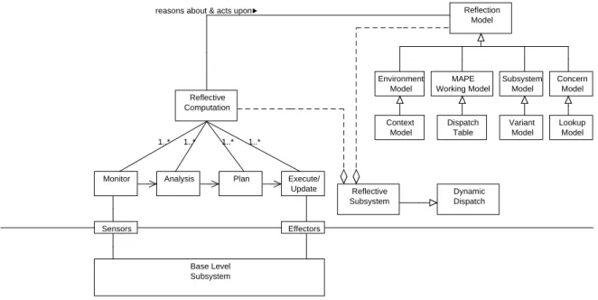
The context-aware composition in principle is a reflective subsystem. It reflects on the behavior and structure of a managed product line (base level subsystem) by selecting best-fit components based on varying context attributes. We use FORMS primitives [65] to describe the context-aware composition as a reflective subsystem. As shown in Figure 5, the context-aware composition reflective subsystem is compose of two basic elements: reflective computation and reflection model. The reflection model element represents knowledge needed by the reflective computation elements to analyze, reason about and plan actions to adapt the managed subsystem. The reflective computation element monitors and adapts a managed subsystem with the help of monitor, analyze, plan and execute components.

A monitor component of the context-aware composition AE monitors a base level system (product line) for context attributes and other system properties. The monitoring is performed using sensors provided by the base level subsystem. The monitor component and sensors correspond to probes and gauges in rainbow framework [27]. The monitored data is forwarded to the analysis component. The analysis component analyzes patterns and structures of the monitored data, performs additional measurements, if needed, and derives a proposal for adaptations. The recommendations (analysis results) are forwarded to the plan component. The analysis and plan components work in close cooperation with each other to prepare an adaptation plan to adapt or manage the underlying base level subsystem. The plan devised by the analysis and plan component consists of recommendations for selecting best-fit components from the dispatch table. Once a plan is ready, it is forwarded to the execute component. The execute component then uses effector(s) provided by the underlying subsystem to run the plan. The plan is executed by binding or rebinding best-fit component variants to compose a new product or adapt an existing product, respectively. The binding and rebinding decisions (plan) made by the plan component often have a greater impact on the base level subsystem and may require further changes, for instance, component reconfigurations and changes in data representations. Such changes may need additional behavior to be planned for, calling the analyze and plan

Reflective Computation Concern Model Subsystem Model Environment Model MAPE Working Model Reflection Model reasons about & acts upon

Reflective Subsystem Dispatch Table 1..* 1..* 1..* 1..* Sensors Effectors Base Level Subsystem Dynamic Dispatch Execute/ Update Plan Analysis Monitor Variant Model Lookup Model Context Model

Figure 5: Conceptual View of Context-aware Composition with FORMS Primitives.

components to further analyze the dependencies and change impact and derive a plan that mitigates possible risks, if any.

Maintaining a self-representation is vital for a reflective subsystem [43] to reason about and act upon the system itself. Being a reflective subsystem, the context-aware composition uses reflection models to maintain a representation of a managed product line (base level subsystem), its environment and properties of interest. The reflection models are causally connected to the product line and are used by the MAPE components (reflective computations) to reason about and act upon the product line, i.e., manage runtime variations and evolution in the product line. The causal connection between two entities implies that a change in one of the two entities leads to a corresponding change or effect upon the other.

As shown in Figure 5, the context-aware composition activity maintains and uses four reflection models: 1) context model, 2) dispatch table model, 3) variant mode and 4) lookup model. The Context Model, a subtype of environment model, maintains a representation of a product line context, i.e., operating environment in which the products are deployed. The Dispatch Table model is a specialized form of a MAPE working model. It contains indexes of the product line’s best-fit components and component variants for a set of distinguished call contexts. The Variant Model maintains a representation of all the managed product line components and component variants. The context-aware composition looks up the best-fit component variants and dynamically binds and invokes them based on the product line’s goals and contexts. The lookup process is controlled by and modeled in the Lookup Model.

3.2.3 Online Learning

The online learning activity is an implementation of a machine learning algorithm that operates at runtime to optimize the dispatch table used by the context-aware composition activity. The knowledge in the dispatch table comes from the offline training activity. The offline training is likely to be imperfect and may lead to errors or suboptimal information in the dispatch table. The errors are caused by factors such as faulty training data and measurements. Moreover, a product line may evolve in its core assets, variants, and context. Such evolution in a product line may invalidate dispatch table and other reflection models used by the context-aware composition. Using an invalid dispatch table, the context-aware composition is likely to result in invalid or suboptimal products that fail to adapt and keep with the evolution in a product line. To that end, the ASPL variability handling mechanism introduces the online learning activity.

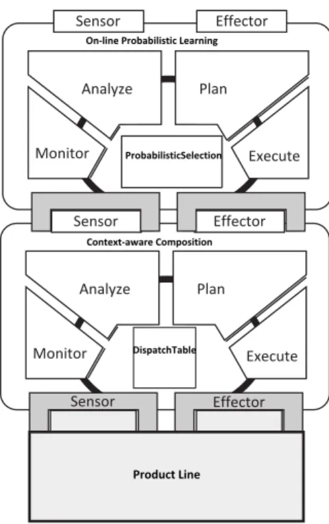
As shown in Figure 6, the online learning is implemented as an autonomic element and operates on top of the context-aware composition. The online learning AE adapts the knowledge base used by the context-aware composition AE by providing new knowledge to the aware composition’s knowledge base. The context-aware composition AE further adjusts behavior and structure of the underlying product line.

Monitor Execute Analyze Plan Sensor Effector Effector Sensor Monitor Execute Analyze Plan Sensor Effector Context-aware Composition On-line Probabilistic Learning

ProbabilisticSelection

DispatchTable

Product Line

Figure 6: On-line learning and Context-aware composition

The online learning AE operates in three phases: 1) instrumentation, 2) monitored execution and 3) learning. The instrumentation phase is initiated when an instrumentation monitor senses that the context-aware composition is activated. The online learning AE preempts the context-aware composition AE and takes control of the context-aware composition. The instrumentation monitor calls instrumentation analysis to investigates which components the composition activity should compose. The analysis results are used by the instrumentation plan component to derive a plan to reflect on the context-aware composition AE. The plan is derived based on a learning strategy or algorithm implemented by the online learning AE. The current implementation of the ASPL variability handling mechanism implements a probabilistic learning strategy. The probabilistic learning strategy operates by intercepting the context-aware composition and replacing optimal variants with suboptimal variants. The replacement is made based on a probability function that invokes suboptimal variants, instead of the best-fit variants from the dispatch table.

The plan made by the instrumentation plan component is forwarded to the instrumentation execute component. The instrumentation execute component runs the plan by deriving a product composed of suboptimal components. The online learning then enters into monitored execution phase. In this phase, a monitor component records the learning goal dependent properties of the suboptimal variants that got selected in place of the optimal variants. After monitoring the performance of the suboptimal variants and recording all properties of interest, the online learning AE moves into the third phase, the learning. In the learning phase, a learning analysis component analyzes monitored properties. The monitored properties, such as execution time, of suboptimal variants, are compared with the earlier known best-fit or optimal variants. If a suboptimal variant outperforms the earlier known so-called best-fit component variant, the learning plan component derives a plan to replace the earlier known best-fit variant with the newly found best-fit variant. The online learning AE executes the plan and replaces the earlier known best-fit variant(s) with the newly found best-fit variant(s). The plan is executed with the help of an effector provided by the context-aware composition AE.

4

Evaluation

To evaluate the ASPL variability handling mechanism, we conducted three experiments described as follows. The experiments were performed with variability across three dimensions, context variability, model variability (variations in dispatch mechanism), and environment variability. The context variability was modeled by varying context attribute values. We define context attribute as a property attached to a composition context (relevant for some qualities of the composed system). A context attribute and its value together form an attribute-value pair, for instance, size=10, 000,

here size is a context attribute and 10,000 is a value of the context attribute size.

The model variability was realized by varying knowledge representations and dispatch mechanisms used in the context-aware composition activity to compose a product. For the environment variability, we did not explicitly model any change in a product line’s environment. We rather tested an online learning mechanism that enables a product line to learn and adapt itself when a product line’s environment changes or diverges, at runtime, from the environment specified at design time.

4.1

Experiment 1: Context Variations

The first experiment was conducted to demonstrate and evaluate the ASPL variability handling mechanism under context variations. We implemented three example product lines for the experiment: 1) Matrix Multiplication, 2) Sorting and 3) Graph algorithms. Following is a detailed description of these example product lines and how we used them to evaluate the ASPL variability handling mechanism under context variations.

4.1.1 Matrix-Multiplication Product Line

Matrix-Multiplication (MM), as the name indicates, is a product line of matrix multiplication applications. Each product in the MM product line takes two square matrices of size N and returns their product matrix as a result. The MM product line is composed of a single core component with four variants. The core component is a generic matrix multiplication algorithm, and the four variants are four different algorithm implementations: 1) Inline, 2) Baseline, 3 Recursive and 4) Strassen. Details about these algorithms are beyond scope here and can be found in the relevant literature.

We used the MM product line to evaluate the ASPL variability handling mechanism under context variability. The context variability was modeled by varying values of three context attributes of the input matrices. The three context attributes were: size, density and data structure representation. The context attribute size was varied with values ranging from 1 to 1024, with a stride of 16. The context attribute density was varied with two distinct variations: sparse and dense. The density of a matrix is a ratio of non-zero elements to total elements of the matrix. The sparse matrices used in the experiment had O(N)non-zero entries, whereas dense matrices had O(N2)non-zero entries, here N is the size of a matrix. The third context attributed data structure representation was varied with two distinct data structure representations.

Following the ASPL variability handling mechanism, the experiment started with an offline training activity. We identified a set of distinguished call contexts and component variants. The variations in three context attributes, size, density and data structure representation, for the two input matrices altogether resulted in 1024/16× (22) × (22) = 1024 distinguished call contexts. The four component variants (matrix multiplication algorithms) with 4 possible matrix data structure conversions (convert m1 to the alternative representation, convert m2 to the alternative

representation, convert both or none) resulted in 4∗4=16 variants. Each of the 16 variants was invoked against a set of 1024 distinguished contexts. Execution for all the 16 variants was monitored and analyzed for an optimization goal, and the variant with best results for the optimization goal was tagged in the dispatch table with its corresponding best data structure conversion. The optimization goal was performance optimization and performance was measured in terms of execution time taken by a variant to multiply the two input matrices.

After offline training, we tested the context-aware composition part of the ASPL variability handling mechanism. For this, we triggered product engineering process of the MM product line under variable context attributes (matrix size, data density, and data structure). The context-aware composition AE probed each call context with the help of a monitor component, analyzed the context attributes and composed a matrix-multiplication product with a best-fit variant for the given context. The best-fit variants for the given call contexts were determined from the dispatch table prepared as a result of the offline training. The product composed as a result of the context-aware composition was named SPLProduct. For each call context, we monitored the execution time taken by the SPLProduct to multiply the two input matrices.

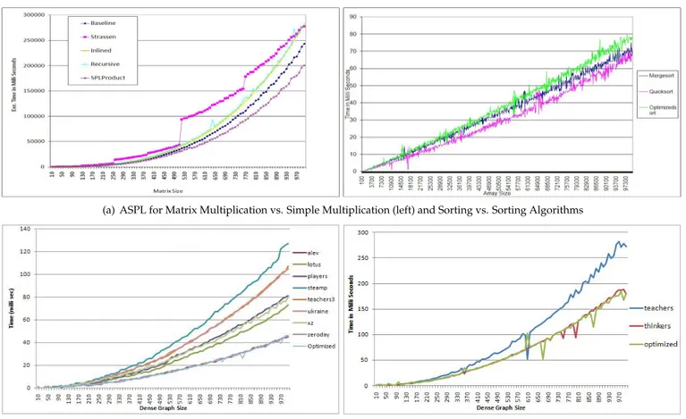
To evaluate the performance of the ASPL variability handling mechanism for the performance optimization goal, we compared the execution time taken by the SPLProduct with four other products that did not use the ASPL variability handling mechanism. Each of the other four products is derived by selecting one of the four variants (Inline, Baseline, Recursive and Strassen) and is named based on the chosen variant. Figure 7(a) depicts execution time taken by the SPLProduct in comparison with the four other products. The x-axis in the figure represents the size of the square matrices and the y-axis marks execution time taken by different products. As shown in the figure, the ‘SPLProduct’ composed using the ASPL variability handling mechanism, outperforms all other products. This indicates that the ASPL variability handling mechanism does not only enable a product line to manage context

variations but also results in a self-optimizing product that outperforms products derived without using the ASPL variability handling mechanism.

(a) ASPL for Matrix Multiplication vs. Simple Multiplication (left) and Sorting vs. Sorting Algorithms

(b) ASPL for DFS vs Different DFS Algorithms (left) and Transitive Closure with Optimized SCC ASPL Product

Figure 7: Evaluating the ASPL variability handling mechanism for context variations

4.1.2 Sorting

Sorting is the second product line developed to evaluate the ASPL variability handling mechanism under context variability. Each product in the sorting product line reads an array of integers and returns a sorted array as a result. The core component of the sorting product line is a sorting algorithm with two variants, Mergesort and Quicksort. The variants are the implementation of the data sort algorithms mergesort and quicksort, respectively. Details about these algorithms are beyond scope here and can be found in the relevant literature.

Following the ASPL variability handling mechanism, the product line was first trained in offline mode. For offline training, the context variability was realized by varying values of the context attribute array-size. The array-size was varied with values ranging from 100 to 10,000 with a stride of 100. Both the mergesort and quicksort variants were invoked against each distinguished array size (call context). The performance of each variant was monitored and analyzed for an optimization goal, and the variant with the best performance was tagged in a dispatch table. For the sorting product line, we considered only one goal, performance optimization. The performance of each variant was measured in terms of execution time required to sort the input array.

With the completion of the offline training, the context-aware composition AE of the ASPL variability handling mechanism was ready for product instantiations. To test and evaluate it under context variability, we provided it with variable contexts attributes. For each call context, the context-aware composition AE probed the context attributes with the help of a monitor component, analyzed the context attributes and composed an array sorting product with a best-fit variant.The best-fit variants for the given call contexts were found from the dispatch table prepared as a result of the offline training. The product composed as a result of the context-aware composition was named ‘Optimizedsort’.

To evaluate the ASPL variability handling mechanism for performance, we compared the execution time taken by the Optimizedsort product with two other products, namely Mergesort and Quicksort. The mergesort and quicksort products use the mergesort and quicksort algorithms, respectively. Moreover, these products are derived using

traditional product line engineering approach and did not use the ASPL variability handling mechanism. As shown by a graph on the right side of the Figure 7(a), the overhead of probing the context attributes and lookup for best-fit variant allowed the mergesort and quicksort products to outperform the Optimizedsort product. Based on results from this experiment, we conclude that in performance critical systems, the ASPL variability handling mechanism may suffer from delays in context monitoring, analysis, and knowledge lookup operations. Thus, more optimized and efficient means are needed to improve the performance of the ASPL variability handling mechanism.

4.1.3 Graph Algorithms

Graph Algorithms (GA) was the third example product line developed to evaluate the ASPL variability handling mechanism under context variability. The GA was, in-fact, a product line of five product lines of graph algorithms. The five product lines were implementations of five graph algorithms, namely Depth First Search (DFS), Breadth First Search (BFS), Connected Components (CC), Strongly Connected Components (SCC) and Transitive Closure (TC). Details about the graph algorithms are out of scope and can be found in the relevant literature.

The core component of each of the GA product line was a graph algorithm with eight variants. The variants were different implementations of the graph algorithm and were contributed by student groups from a two years master program in software engineering. For instance, a core component of the DFS product line was a generic depth first search graph algorithm, and the eight variants were the eight different implementations from the student groups.

All the example product lines in the GA product line were developed to evaluate the ASPL variability handling mechanism under context variability. For each product line, context variability was modeled by varying two graph attributes, graph size (number of graph nodes) and density. The graph size was changed from 1 to 1024, with a stride of 16. The context attribute graph density was varied with two distinct variations, sparse and dense.

To begin the evaluation, we started with the Depth First Search product line and performed offline training. A set of distinguished call contexts and component variants for the DFS product line were determined. The variations in the graph size and density resulted in 1024/16×2=128 distinguished call contexts. Each of the eight variants of the DFS product line was invoked against each differentiated call context. The performance of each variant was monitored and analyzed for an optimization goal, and the variant with the best performance was tagged in a dispatch table. For the DFS product line, we considered only one goal, performance optimization. The performance was measured in terms of execution time taken by a DFS variant to traverse the input graph.

After offline training, we tested context-aware composition part of the ASPL variability handling mechanism. For this, we triggered product engineering process of the DFS product line under variable context attributes (graph size and density). The context-aware composition AE probed the given context attributes with the help of a monitor component, analyzed them and composed a DFS product with best-fit variants for given call contexts. The best-fit variants were determined from the dispatch table prepared as a result of the offline training. The product composed as a result of the context-aware composition was named ‘Optimized’.

To evaluate the ASPL variability handling mechanism for the performance optimization goal, we compared the execution time taken by the Optimized product with eight other products that did not use the ASPL variability handling mechanism. Each of the other eight products was derived by selecting one of the eight variants of the DFS algorithm produced by the student groups and were named accordingly. A graph on the left side of the Figure 7(b) depicts execution time taken by the Optimized product in comparison with the eight other products. The x-axis of the graph represents dense graph size, whereas the y-axis marks execution time to traverse the dense graphs. As shown in the figure, the ‘Optimized’ product composed using the ASPL variability handling mechanism, outperformed all other products. This indicates that the ASPL variability handling mechanism does not only enable a product line to manage context variations but also results in a self-optimizing product that outperforms products derived without using the ASPL variability handling mechanism.

The Optimized DSF product was then used in the Strongly Connected Components (SCC) product line. The SCC product line was a product line of graph algorithms to compute strongly connected components in a directed graph. For the SCC product line, we performed offline training and context-aware composition using the same experimental setup as used in the DFS product line. An ‘Optimized’ SCC product was derived as a result of the context-aware composition activity. The optimized SCC product was used by yet another product line, the Transitive Closure (TC) product line.

The TC product line was a product line of graph algorithms to compute transitive closure of given graphs. The core components of the TC product line was a generic transitive closure algorithm with two variants, namely ‘teachers’ and ‘thinkers’. The variants were different implementations of the transitive closure graph algorithm, contributed by student groups from a two years master program in software engineering. We applied the ASPL variability handling mechanism to the TC product line to evaluate its performance. The offline training and context-aware composition activities of the ASPL variability mechanism were performed with same experimental setup, goal and

Figure 8: Evaluating the ASPL variability handling mechanism for model variations

context variability as used in the DFS product line. An ‘Optimized’ TC product was produced as a result of the context-aware composition activity of the ASPL variability handling mechanism.

To evaluate the performance of the ASPL variability handling mechanism, we compared the execution time taken by the Optimized TC product with two other products. The other products were derived by selecting one of the two variants of the TC core component and were named accordingly as ‘teachers’ and ‘thinkers’. Moreover, the teachers and thinkers products were derived using traditional product line engineering approach and did not use the ASPL variability handling mechanism. As shown by a graph on the right side of the Figure 7(b), the Optimized product composed using the ASPL variability handling mechanism, outperforms the two other products. This shows that the ASPL variability handling mechanism does not only enable a product line to manage context variations but also results in a self-optimizing product that outperforms products derived without using the ASPL variability handling mechanism.

Based on combined results from the three example product lines, we conclude that the ASPL variability handling mechanism enables traditional software product lines to manage context variations at runtime. Moreover, the ASPL approach (the ASPL variability handling mechanism) results in context-aware self-configuring and self-optimizing products that are capable of monitoring their contexts and adapting themselves in response to changes in their context attributes.

4.2

Experiment 2: Model Variations

The second experiment was performed to demonstrate the working of the ASPL variability handling mechanism with variations in the models used to represent the knowledge base. Three model variants, 1) dispatch table, 2) support vector machine (SVM) and 3) probabilistic dispatch, were used to model knowledge and realize dynamic dispatch mechanism for the context-aware composition of products. The three model variants resulted in three variants of the ASPL variability handling mechanism.

The dispatch table model was defined as a result of offline training. It uses a table to index best-fit variants of a product line against a finite set of distinguished contexts. A dispatch function then maps a given call context to the closest context captured in the table to retrieve best-fit variant(s) for the given system context.

The SVM model was realized by adopting Support Vector Machine (SVM) classifier method to learn optimal variants for given call contexts. A finite set of distinguished call contexts and best-fit variants for these call contexts were fed into an SVM machine learner. The learned SVM classifier was then used to retrieve best-fit component variants for any runtime call context.

The probabilistic dispatch model was defined on the basis of a probability table. For each product line component and component variant, probabilities of getting selected in a product configuration were recorded in a probability table. The probabilities were computed, during offline training, based on the components and variants performance for a particular goal. The variants with better performance were assigned higher probabilities and vice versa. The probability table was then used by the context-aware composition part of the ASPL variability mechanism to select variants for product configuration. Unlike the simple dispatch table model that always returned best-fit variants, the probabilistic dispatch model chose variants probabilistically based on probabilities recorded in the probability table.

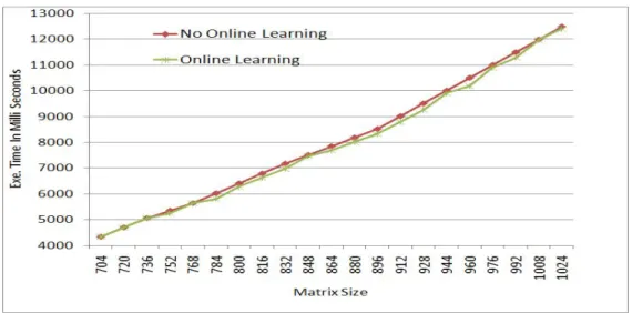
Figure 9: Evaluating the ASPL variability handling mechanism for environment variations

We tested the use of the above-described model variants. The tests were conducted using the matrix-multiplication product line, described in Section 4.1.1, with dense matrices of varying sizes and dense representation. The figure 8 shows performance results for all the three model variants. As shown in the figure, the SVM model based ASPL variability handling mechanism performed best. The Dispatch Table based ASPL variability handling mechanism was not far behind from the SVM based variant. Both the SVM and dispatch table based variants clearly outperformed the probabilistic dispatch model based variant. This came as no surprise because the probabilistic dispatch model selects and binds variants probabilistically and keeps on selecting non-optimal variants now and then.

4.3

Experiment 3: Environment Variations

The third experiment was performed to demonstrate and evaluate the ASPL variability handling mechanism under environment variability. For this, we did not model any explicit change in environment. Instead, we implemented a probabilistic online learning strategy that enables a product line to learn and adapt itself to variations in the product line environment. A runtime change in a product line environment may invalidate the knowledge base used by the ASPL variability handling mechanism to compose context (environment) aware product. The online learning manages such environment variations by optimizing the knowledge base with the removal of obsolete information and addition of new knowledge.

To perform this experiment, we reused the matrix-multiplication example product line from experiment one. The offline training for the matrix-multiplication was already conducted in experiment one. Thus, we just reused the already prepared dispatch table. Continuing with the context-aware composition activity, we derived two products. The first product was derived with no online learning activity whereas the second product was derived with the online learning activity. As described in Section 3.2.3, online learning activity was realized as an autonomic element that operates on top of the context-aware composition. The online learning AE wad defined by implementing a probabilistic online learning strategy. Instead of selecting a best-fit variant, the probabilistic online learning strategy chose the second best variant. The selection of second best variants was guided by the probabilistic dispatch model used in Experiment two.

To evaluate online learning part of the ASPL variability handling mechanism, we recorded and compared the performance of the product derived using online learning activity with the product that was derived with no online learning. As shown in Figure 9, The product composed with online learning has a slight advantage over the product composed without online learning. The difference between the two products is, however, marginal. This endorses credibility of our simple offline training activity that is a first and foundational step of the ASPL variability handling mechanism. Based on results of this experiment, we conclude that the online learning part of the ASPL variability handling mechanism enables traditional SPLs to improve quality of their products by optimizing their performance at runtime. Moreover, it also empowers traditional SPLs to manage runtime changes in the environment and other context attributes by optimizing the knowledge base.

5

Related Work

Dynamic software product lines (DSPL) [15, 31, 33, 60, 39, 22], variability management [61, 56, 10, 39], context-aware computing [51, 28, 36, 34, 25] and machine learning [16, 49, 57, 42, 24, 23, 32, 55, 38] are the key research communities related to the ASPL approach and the ASPL variability handling mechanism. We introduce and discuss some of the major contributions from each of the related research community.

Dynamic Software Product Lines (DSPL)The DSPL community aims to design and develop dynamic software product lines (DSPLs) whose products can adapt themselves to changes in user needs and operating environments [33, 15]. Hallsteinsen et al. [33] motivated the need for developing DSPLs and identified a set of essential and optional properties of dynamic software product lines. The essential properties include dynamic variability, (re-)configuration and ability to deal with unexpected changes. The optional properties include context-awareness, autonomic or self-adaptation, and automatic decision making. The ASPL approach satisfies almost all the required and optional properties of DSPLs. The ASPL variability mechanism supports context-awareness and results in dynamically reconfigurable products with self-managing characteristics to manage variations in user needs and operating environments.

Cetina et al. [14] proposed a mixed DSPL approach to develop autonomic self-managing software systems. The mixed DSPL approach is a combination of connected and disconnected DSPLs. The distinction between connected and disconnected DSPLs is made on the basis of who triggers and controls product line adaptations. In a connected DSPL, it is a product line that triggers and controls adaptations, whereas, in disconnected DSPLs, the products themselves trigger and control their adaptations. The mixed DSPL approach produces scenario-aware configurable products, and depending on a scenario may switch from connected to disconnected DSPL approach. The ASPL approach is identical to the mixed DSPL because it involves both connected and disconnected scenarios. The ASPL products may have internal (disconnected) adaptations as well as external (connected) adaptations. In an internal adaptation, the ASPL products themselves adapt to changes, independent of the ASPL variability handling. Whereas, the external adaptations are triggered and controlled by the ASPL variability handling mechanism.

There exist several feature models based approaches to design and develop DSPLs [39, 60]. Lee and Kang [39] presented a feature-oriented approach to manage variations in a product line. The presented approach analyzes a product line in terms of features and features’ bindings. The feature binding analysis serves as a key design driver to identify and manage variation points. Dynamically reconfigurable core assets are developed based on the feature binding analysis. A dynamic re-configurator manages reconfiguration activities including when to reconfigure, what to reconfigure and how to reconfigure. A major issue with the presented approach is that it does not specify any mechanism to deal with unexpected changes in product line’s context, requirements and to incorporate new features into a product line. In the ASPL approach, we simply model product features as variants, and let the ASPL variability mechanism to bind variants dynamically. We plan to use and take advantages of the feature binding analysis work in future. We also plan to investigate how the feature binding analysis and the online learning mechanism of the ASPL approach can be combined to take care of unexpected changes and new features.

Trinidad et al. [60] proposed another feature-oriented model to design and develop dynamic software product lines. The model comprises four steps: 1) define a core architecture by identifying core (essential) product line features, 2) transform the core architecture into a dynamic architecture with non-core variable features, 3) develop a configurator, and 4) derive a product by selecting core and non-core features (variants). The configurator component developed in step three provides dynamic behavior for a product line, similar to the re-configurator component in the Lee and Kang’s approach [39]. It dynamically receives feature activation/deactivation requests, validates them and activates or deactivates features accordingly. In the ASPL approach, the context-aware composition works as a dynamic configurator to activate and deactivate components and their variants.

Gomaa and Hussein [31] described a reconfiguration patterns based approach to design and develop DSPLs. The approach named Reconfigurable Evolutionary Product Family Life Cycle (REPFLC) consist of three major activities: 1) product family engineering, 2) target system configuration and 3) target system reconfiguration. The three activities are described on the abstract level and lack detail description needed for implementation. Moreover, the REPFLC approach lacks in autonomic mechanism to trigger adaptation or reconfiguration of products. It requires a user to specify changes in product configurations to reconfigure a product at runtime. The ASPL approach comes with a detailed description of the variability handling mechanism that forms a built-in mechanism to trigger and control product reconfigurations.

Context-Modeling and Context-Aware Computing Context information is one of the leading factors that control design decisions to design and develop self-adaptive software systems. The current computing environments require software systems to be context-oriented and adaptable to changing context and situations. Context-Oriented Programming (COP) is a novel programming approach aimed to facilitate the development of context-oriented software systems. It allows developing software systems with gaps or open-terms that are later filled by selecting

pieces of code from a repository of candidate code components. The selection of candidate code components is guided by execution context and product goals [36]. The primary objective is to fill the gaps with best-fit code variants. This is what the ASPL does by dynamically dispatching best-fit variants to the variation points.

One of the challenges to develop context-aware systems is how to model and represent context information [25]. To address the challenge, a number of context modeling and reasoning techniques [8, 12, 17, 20, 29, 30, 63, 44, 53] have been proposed over the years. Bettini et al. [9] discussed the problem of uncertainty in context information and described several widely used techniques to model and represent context information. In the ASPL approach, at present, we use a simple key-value model [53] to represent the context information. But in future, we plan to investigate and use other context modeling and reasoning methods.

The context-aware composition activity of the ASPL variability handling mechanism combines software composi-tion with software optimizacomposi-tion. Both software composicomposi-tion and optimizacomposi-tion are currently being explored almost in isolation in two different scientific communities. Software composition is being treated as a general-purpose comput-ing problem that can be addressed in a number of ways such as meta and generative programmcomput-ing, configuration, and (self-)adaptation, software architecture, and component systems. Whereas, optimization is usually considered as a problem of high-performance computing and compiler construction. The system or program optimization problem is commonly addressed by techniques such as auto-tuning, scheduling, parallelization, just-in-time compilation, runtime optimizations, and performance prediction.

Automatic program specialization has been a great concern in the composition community for many years; the cost of generality is sometimes too big to be acceptable. Hence the interest is in efficient specialization for specific applications. For object-oriented languages, the work of Schultz et al. [54] demonstrates how advice from developers may be used to specialize applications automatically.

Domain-specific library generators achieve adaptive optimizations by using profile data. The profile data is collected during offline training processes to tune key parameters, such as loop blocking factors to adapt to, e.g., cache sizes. This technique is used for both generators that target sequential and parallel libraries, for instance, ATLAS [66] for linear algebra computations, and SPIRAL [45] and FFTW [26] for Fast Fourier Transforms (FFT) and signal processing computations. With its concept of composition plans computed at runtime, FFTW also supports optimized composition for recursive components. SPIRAL is a generator for library implementations of linear transformations in signal processing. Given a high-level formal specification of the transformation algorithm and a description of the target architecture, SPIRAL explores a design space of alternative implementations by combining and varying loop constructs, and produces a sequential, vectorized or parallel implementation combining fastest versions for the target platform.

Li et al. [40] implemented a library generator that uses dynamic tuning to adapt a library to a target machine. They used several machine parameters (such as cache size, the size of the input and the distribution of the input) as input to a machine learning algorithm. The machine learning algorithm is trained to pick the best algorithm for any considered scenario. In contrast to the domain-specific auto-tuning systems, the ASPL approach is general-purpose, and its optimization scope is not limited to libraries, but can also be applied to complete applications and arbitrary optimization goals.

Machine Learning Learning is one of the key activities of the ASPL variability handling mechanism. Machine learning is viewed as one of the best options to achieve intelligent computing systems. A large number of machine learning methods [16, 3, 49, 57, 42, 24, 23, 32, 55, 38] have been proposed to support self-managing and self-adaptive software systems. At present, the ASPL approach uses a simple probabilistic learning method to realize its online learning activity. In future, we plan to investigate other learning methods, particularly the methods described below.

Reinforcement learning (RL) is a widely used [24, 57, 42, 59, 58, 52, 62] and well acknowledged learning approach in autonomic computing. In its simple form, it involves a single agent that learns to optimize a system’s interactions in an uncertain environment. The learning agent receives feedback or reward from the system (environment) that guides the learning mechanism in the right direction. MAPE-K [37] is one of the most widely used approaches to design and develop self-adaptive software systems. The MAPE-K implements a feedback loop driven by reflective models and computations that move a system from current state to the desired state. This makes RL to be a potential candidate to implement a MAPE-K loop by learning an adaptation policy.

Tesauro et al. [58] reported two significant advantages of RL approach to realize self-managing system. First, it does not require an explicit model of the computing system being managed. Second, it recognizes a possibility that a current decision may have delayed consequences for both future rewards and future observed states. However, the RL in its pure form suffers from scalability and poor online training performance.

An alternative approach to RL is hybrid reinforcement learning. Introduced by Tesauro et al. [58], the hybrid reinforcement learning combines strengths of the RL and queuing models to improve the performance of the simple reinforcement learning method. Dowling et al. [24] presented another alternative approach, collaborative reinforcement learning (CRL). The CRL is a multi-agent, decentralized extension of the RL method to support online learning. The

CRL method aims to learn an online coordination model that behaves autonomically in a decentralized setting. It uses multiple learning agents that collaborate to share information with their neighbors. The participating agents dynamically leave, join and establish connections with their neighbors. Through the collaboration of multiple agents, the CRL method models a decentralized and robust multi-agent learning mechanism that can work in highly dynamic and uncertain environments.

6

Conclusions and Future Work

This report describes a work in progress to develop an Autonomic Software Product Lines (ASPL) approach. The ASPL is a dynamic software product line engineering approach[33] to design and develop families of self-adaptive software systems.

A key characteristic of the ASPL approach is a dynamic variability handling mechanism that enables traditional software product lines to reason about their contexts and dynamically reconfigure their products at runtime. The ASPL variability handling mechanism is composed of three core activities: 1) context-profiling, 2) context-aware composition, and 3) online learning. Context-profiling is a design time activity performed offline to prepare a knowledge base. The knowledge base maps a finite set of call contexts to best-fit components or component variants. The context-aware composition is a product engineering activity performed to derive a new product or to adapt a product in execution. It monitors a product’s call context and uses the knowledge base, prepared by context-profiling, to configure or reconfigure a product with best-fit variants. The knowledge base used by the context-aware composition is likely to become obsolete due to changes in goals and context evolution. The online learning activity optimizes the knowledge base by implementing a machine learning method at runtime.

The ASPL variability handling activities are modeled and implemented as autonomic elements (AEs) [37]. The AE models a reflective system [5] that reflects adaptation actions on a managed system. The three activities implemented as autonomic elements together form a simple yet powerful mechanism to manage changes in a product line’s requirements, business goals, and environment.

We performed three experiments to evaluate the ASPL variability handling mechanism. The experiments were aimed to demonstrate the feasibility of the approach. Based on combined results from these experiments, we conclude that the ASPL variability handling mechanism forms a promising approach that enables traditional software product lines to manage variations in their context.

The ASPL is yet on initial stage, far from being complete with several intriguing challenges ahead. We plan to investigate further how to improve the three activities of the ASPL variability handling mechanism, including context prediction and sensing, training setup, online sensing and reasoning. Besides, we will continue to further verify the ASPL approach and the online learning activity of the ASPL variability handling mechanism. We plan to intentionally seed errors in the knowledge base and test the online learning activity to optimize the knowledge base gradually by detecting and removing these errors. These experiments aim at verifying the robustness of the ASPL variability handling mechanism. The future work also includes improved development support, for instance defining a process for offline training, for the ASPL variability handling mechanism.

References

[1] An Architectural Blueprint for Autonomic Computing, White Paper, 2006.

[2] N. Abbas, J. Andersson, and W. L ¨owe. Autonomic Software Product Lines (ASPL). In Proceedings of the Fourth European Conference on Software Architecture: Companion Volume, pages 324–331. ACM, 2010.

[3] M. Amoui, M. Salehie, S. Mirarab, and L. Tahvildari. Adaptive Action Selection in Autonomic Software Using Reinforcement Learning. In Proceedings of the Fourth International Conference on Autonomic and Autonomous Systems, pages 175–181. IEEE Computer Society, 2008.

[4] J. Andersson and J. Bosch. Development and use of dynamic product-line architectures. IEE Proceedings Software, 152(1):15–28, February 2005.

[5] J. Andersson, R. de Lemos, S. Malek, and D. Weyns. Reflecting on self-adaptive software systems. In Software Engineering for Adaptive and Self-Managing Systems, 2009. SEAMS ’09. ICSE Workshop on, pages 38 –47, may 2009. [6] J. Andersson, M. Ericsson, C. Kessler, and W. L ¨owe. Profile-Guided Composition. In Proceedings of the 7th