i
Faculty of Engineering
Department of Industrial Management and Logistics Division of Production Management
Determination of Batch-Sizes
A case-study in the process industry.
Master Thesis in Production Management – MIOM01
Spring 2018
Authors
Simon Gottfridsson
Viktor Farbäck
Supervisors
Johan Marklund, LTH
Fredrik Johansson, The Company
Examiner
ii
Acknowledgements
We would like to thank everyone that have in any way been a part of this thesis. Special thanks are extended to Johan Marklund, our professor and supervisor at Lund University for all his time and valuable inputs and to Fredrik Johansson, our supervisor at the company who have been a constant support.
Our gratitude is also extended to all lecturers and students that have made our time at the mechanical engineering program, and in turn the supply chain management program at LTH, to valuable experiences.
iii
Abstract
Title
Optimization of batch sizes, A case-study in the process industry.
Course
Degree Project in Production Management – MIOM01
Authors
Simon Gottfridsson and Viktor Farbäck
Supervisor
Johan Marklund, LTH & Fredrik Johansson, the company.
Background and Research question
The company have a complex product portfolio and production facility. Currently, the batch sizes in production are based on experience and is not based on any cost analysis. The central organization have recently put more emphasis on the batch sizes, especially in a context of increasing the efficiency of the packaging lines. The company wishes to investigate the batch sizes and analyze the consequences of implementing a method to calculate batch sizes from a cost perspective.
Methodology
The chosen research method is a balanced approach which incorporates both qualitative- and quantitative research. Interviews and archive analysis was used to develop an
understanding of the problem and obtaining data for a quantitative analysis. The research took place at the company and the data was collected from the company’s IT systems.
Theoretical Framework
Theory relevant to the problem at hand was first studied and is presented in the report. This theory is well-established in operations research and is used as both a foundation to analyze the current situation as well as a base for suggestions of how to solve the company’s
problems.
Conclusion
The EOQ model was chosen as a suitable theoretical model for the company. During the analysis, several findings were made regarding the current approach of determining costs and managing the inventory. The current approach of determining batch sizes encourages a reactionary way of thinking for operational planners where the most important SKUs are shown most regard due to pressure from top management. The current way of calculating safety stock have also been shown to greatly discourage an increase in batch sizes, even though an increase could both be cost-effective and increase efficiency in production. Hence, a new theoretically sound method to calculate safety stock s suggested.
The report presents an approach that takes cost, the perishability of products and operational constraints into account and provides the company with an Excel based decision making tool.
Keywords
iv
Content
Acknowledgements ... ii Abstract ... iii 1 Introduction ... 1 1.1 Background ... 1 1.2 Problem Description ... 1 1.3 Purpose ... 2 1.4 Delimitations... 2 2 Methodology ... 3 2.1 Research purpose ... 3 2.2 Research Design ... 32.2.1 Company case study ... 3
2.2.2 Modelling ... 3 2.3 Research Techniques ... 4 2.4 Problem Description ... 4 2.4.1 Interviews ... 4 2.4.2 Observations ... 5 2.4.3 Archive analysis ... 5 2.5 Research Approach ... 6 2.6 Research Strategy... 6 2.7 Quality Assurance ... 7 2.7.1 Reliability ... 7 2.7.2 Validity ... 7 2.7.3 Representativeness... 7 2.8 Chosen methodology ... 7 2.8.1 Used Methodology ... 7 2.9 Working procedure ... 9 3 Theoretical Framework ...11
3.1 Strategic levels of organisations ...11
3.2 Sales and Operations Planning ...11
3.3 Enterprise Resource Planning ...12
3.4 Lot Sizing ...13
3.4.1 The Economic Order Quantity ...13
3.4.2 Wagner-Whitin ...15
3.4.3 Silver-Meal ...15
v
3.5.1 Holding Cost ...16
3.5.2 Activity Based Costing ...17
3.5.3 Changeover Cost ...17
3.5.4 Shortage Cost ...17
3.6 (R, Q) Policy ...17
3.7 Service Levels and Safety Stocks ...18
3.8 Yield loss ...19
3.9 Statistical Theory ...19
3.9.1 Linear combinations of stochastic variables ...19
3.9.2 Statistical fitting ...20 3.9.3 𝜒2-test ...20 3.9.4 Kolmogorov-Smirnov test ...21 4 Empirical Context ...23 4.1 Supply chain...23 4.2 Processing ...24 4.3 Packaging ...24 4.3.1 Production Fulfilment ...25 4.3.2 Changeover Process ...25 4.3.3 Line Efficiency ...26 4.4 Warehouse ...27 4.5 Information systems ...28 4.5.1 SAP ...28
4.5.2 Production follow-up tool ...28
4.5.3 MES ...28
4.5.4 Warehouse Management System (WMS) ...29
4.5.5 Business Intelligence software (BI) ...29
4.6 Inventory Control ...29
4.6.1 Batch Size ...29
4.6.2 Service Level...29
4.6.3 Safety stock ...30
4.7 Activities in the Planning Department ...31
4.7.1 Operative planning process ...31
4.7.2 Stock building ...32
4.7.3 Cycle planning of SKUs ...33
4.7.4 Sales and Operations Planning at the Company ...33
vi
5.1 Mathematical Lot sizing ...37
5.1.1 EOQ ...37 5.1.2 Wagner-Whitin ...38 5.1.3 Silver Meal ...38 5.1.4 Chosen Model ...38 5.2 Changeover Cost ...39 5.2.1 Changeover Times ...39
5.2.2 Fixed changeover cost ...40
5.2.3 Variable Changeover Cost ...40
5.2.4 Total changeover cost ...40
5.2.5 Outcome ...41
5.3 Holding cost ...41
5.3.1 Holding cost in today’s operations ...42
5.3.2 Holding cost for an extended internal warehouse ...43
5.4 Demand ...43
5.5 Constraints in Processing ...44
5.6 Statistical analysis related to Perished Goods ...45
5.6.1 Maximum Batch Size ...45
5.6.2 Expected volume of perished goods ...47
5.6.3 Discussion of approaches ...48
5.7 Resulting batch sizes from the model ...48
5.8 Safety Stock ...51
5.8.1 Implication of current setup ...51
5.8.2 A new suggestion ...53
5.9 Effects on finished goods inventory ...56
5.10 Effects on production ...57
5.11 Cycle planning ...59
5.12 Summary ...60
6 Model Outline ...63
6.1 Application of the Model ...63
6.2 Model procedure ...63
6.3 Model procedure to evaluate effects. ...65
6.4 Input Data ...65
7 Discussion ...67
7.1 Sensitivity analysis ...67
vii
7.3 Areas for future improvement ...68
8 Summary and Conclusions ...69
9 Recommendations ...71
viii
List of Figures
Figure 1: The balanced approach to research strategy (Kotzab & Westhaus, 2005, p.20) ... 6
Figure 2: The MRP2 hierarchy (Hopp & Spearman, 2001, p.136). ...12
Figure 3: Level of stock in the system as assumed in EOQ-model (Axäter, 2006) ...13
Figure 4: Example of the wagner-whitin algorithm at work (Axäter, 2006, p.65). ...15
Figure 5. (R,Q) Policy (Axäter, 2006, p.50) ...18
Figure 6: The company’s supply chain in Sweden ...23
Figure 7: Activity distribution for the open time of line X. ...27
Figure 8 stock on hand at the warehouses dated back to January 1, 2017. ...28
Figure 9 The operative planning process ...31
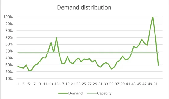
Figure 10: Demand of SKUs produced by line Y throughout the year, and the capacity of the line. ...32
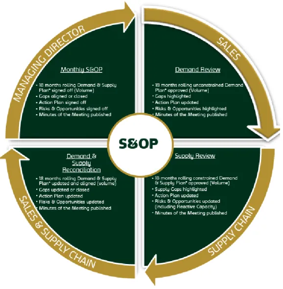
Figure 11: The S&OP process at the company. ...34
Figure 12. Demand for the SKUs on the four lines throughout the year. ...44
Figure 13 Histogram of FE for a SKU. ...45
Figure 14 illustration of risk for perished goods...46
Figure 15. Average batch size per recipe-group. ...49
Figure 16 Average batch sizes on the four studied lines. ...50
Figure 17 cost analysis when deviating from optimum batch size ...51
Figure 18: Histogram of yield loss in percent for Line Y, a negative yield loss means the produced quantity was larger than the planned. ...54
Figure 19: Safety stock for new suggestion and Current setup ...56
Figure 20 Contributions of average stock on hand from the studied lines. ...57
Figure 21: Changes is production time and changeover times at the lines. ...59
Figure 22: Tiers of suggested model ...63
Figure 23: Flowchart of working model procedure. ...64
Figure 24. Illustration of selection of possible batch sizes. ...65
ix
List of Tables
Table 1: Opening hours in production during a week. ...24
Table 2: Average production fulfillment during the last 4 years for the four studied production lines. ...25
Table 3: Average change over times of different recipe groups on one line during 2017 in minutes...39
Table 4: Average changeover times of different SKUs in a recipe group during 2017 in minutes...40
Table 5: The Changeover cost for all recipes in SEK. Each cell in the columns represent one of the recipes of the line. ...41
Table 6: Consequence of constraints on batch size ...44
Table 7 results of MAXQ and expected perishable goods for a selection of SKUs. ...47
Table 8. Average batch sizes for a selection of SKUs...49
Table 9: Last six months service level for the 10 SKUs with highest sales volume, as observed, and the target “stock service level”. ...52
Table 10: Mean and standard deviation of yield losses for the lines in this study, note that it is displayed in units of percent. ...55
Table 11. Calculated parameters for the selection of articles ...58
Table 12. Production time per week ...58
Table 13: The Cycle-planning helper. ...60
Table 14. Data aggregated to evaluate effects on production and finished goods inventory for a selection of SKUs across the 4 lines included in the report. ...65
1
1 Introduction
During the introduction the reader will be introduced to the company and their current situation. The problem will be described, a clear purpose of this thesis, and its delimitations, will be stated.
1.1 Background
The beverage industry has ancient roots. For example, the procedure of refining water, malt, hops and yeast into beer, called Brewing is a complicated process that have been developed by humans for more than 7000 years. (Nelson, 2005)
The project was performed at the request of a company that manufactures beverages, at their production facility in Sweden. The facility produces a multitude of different beverages and packages them to be sold. The company possesses a vast array of brand that are both internationally and locally known. The company wishes to remain anonymous, and shall in this thesis be referred to as “The company”. The names of the production lines and the articles have also been altered in this thesis.
This thesis concerns the manufacturing unit in Sweden which produce drinks for the Swedish market. In total, around 400 unique products are produced in the facility at this time.
1.2 Problem Description
The company currently experience difficulties in the decision-making process regarding ordering quantities along their supply chain. The planning department is responsible for determining the produced batch sizes, but the decisions affect the various departments throughout the supply chain in different ways depending on which KPIs (Key Performance Indicators) the department is evaluated upon. Therefore, the batch sizes in the production are a topic of much interest for the entities in the supply chain and various opinions related to them exist.
Several problematic areas that might be affected by the batch sizes exist. The warehouse management team brings attention to the fact that 40-60% of the company’s finished goods inventory is stored at expensive external warehouses, to which inventory must be
transported. In turn, the production management highlights the low equipment efficiency shown on the production lines and the resulting cost of sourcing goods that cannot be produced on site due to lack of capacity. Sourcing of finished goods and the cost of external warehouses are considered by the departments to be major unnecessary cost drivers.
The planning department currently have an ambition to decrease the total stock and to create good conditions for the production team, to increase their equipment efficiency by reducing the number of change overs. They think this can be done by enhancing the procedure of determining batch sizes in production, an effort that is complicated by the complexity of the company’s large product portfolio and constraints in their production process, as well as the
2
perishability of the finished goods. The planning team is currently guided by SAP to handle the production scheduling of the production lines. SAP suggests a preliminary production schedule with batches that aim to satisfy the demand from the customers, but does not take the costs driven by the batches, into account.
To support the planning team in the batch size determination, as well as in negotiations with the different functions, a model that quantifies the costs associated with the batch sizes have been requested. To increase the understanding of the impacts of decisions, the model is requested to be capable of evaluating the effect of changes to the finished goods inventory and the production
1.3 Purpose
The purpose of this project is to create a quantitative model that takes relevant costs and variables into account when determining the production batch sizes. The objective is also to evaluate the impact the model would have on finished goods inventory and the production capacity.
1.4 Delimitations
To be able to perform the project in the limited time frame, the scope is narrowed down. Firstly, only one of the company’s production facilities is included. Therefore, the scope of the project has been limited to the supply chain and the operations related to this production unit. The ambition to create a model which can be used in the planning process for most products have because of the limited time frame been tested on four of the production lines.
3
2 Methodology
Appropriate research methodology is crucial to clarify how the project will be carried out and for the quality assurance. However, the purpose of the methodology is not to dictate how the work will be executed but rather guide the process of acquiring knowledge from the problem formulation. (Höst, et al., 2006). In this chapter, several key aspects of the methodology will be presented. Motivations are given for the chosen methodology and how quality is assured.
2.1 Research purpose
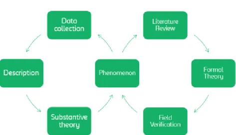
A methodology can have different purposes depending on the goals and characteristics of the project (Höst, et al., 2006). Four different types of purposes are presented by Runesson and Höst (2009), namely exploratory, descriptive, explanatory and improving. The research purpose depends on the knowledge of the studied phenomenon. Exploratory research aims to explore and develop an understanding of the phenomenon. With greater knowledge of the phenomenon, a descriptive research purpose aspires to describe what is happening.
Explanatory research intends to explain the phenomenon. An improving research purpose develop a solution which solves a problem. Thus, the different purposes represent the level of understanding of the problem which increases from little knowledge in an exploratory research purpose to profound knowledge in an improving research purpose (Runesson & Höst, 2009).
2.2 Research Design
A suitable research design must be aligned with the research purpose. Examples of ways to design a research study are through case studies and modelling (Höst, et al., 2006). Kotzab and Westhaus (2005) use the phrase research strategy and outline case studies and
modelling from a supply chain perspective. Christer Karlsson (2016) also explains these strategies from an operations management perspective.
2.2.1 Company case study
Projects which are set out to solve a problem experienced in a manufacturing industry are by its nature a study of a particular case and thus the design of the methods are considered flexible. (Höst, et al., 2006) In this context, flexible means that the questions asked, and the alignment of the study can be altered during the project itself. These studies can include both quantitative and qualitative evidence. They also benefit from multiple sources for these evidence, as well as from a previously set theoretical framework. (Yin, 2014)
2.2.2 Modelling
A model is an abstraction of the reality where un-relevant aspects of the phenomenon are disregarded (Höst, et al., 2006). Modelling of supply chains can relate to quantitative methods such as systems dynamics, agent-based simulation, object-oriented modelling, discrete event simulation, stochastic modelling, optimization problems and queuing networks (Kotzab & Westhaus, 2005). These methods are applied to study how uncertainty and inventory quantities affect the performance of the supply chain (Kotzab & Westhaus, 2005).
4
2.3 Research Techniques
There are several different techniques that can be used for collecting data when studying a particular case. Höst, Regnell and Runesson (2006) especially mention three common techniques, which can be conducted in several ways. These are Interviews, Observations and Archive analysis.
2.4 Problem Description
The company currently experience difficulties in the decision-making process regarding order quantities along their supply chain. The planning department is responsible for determining the batch sizes used in production, but the decisions affect the various departments
throughout the supply chain in different ways depending on which KPIs (Key Performance Indicators) the department is evaluated upon. Therefore, the batch sizes in the production facility is a topic of much interest for all the different entities in the supply chain.
Several problematic areas that might be affected by the batch sizes exist. The warehouse management team brings attention to the fact that 40-60% of the company’s finished goods inventory is stored at expensive external warehouses, to which inventory must be
transported. In turn, the production management highlights the low equipment efficiency seen in some of the production lines and the resulting cost of sourcing goods that cannot be produced on site due to lack of capacity. Sourcing of finished goods and the cost of external warehouses are considered by the departments to be major “unnecessary” cost drivers. The planning department currently have an ambition to decrease the total stock and to create good conditions for the production team, to increase their equipment efficiency by reducing the number of change overs. They think this can be done by enhancing the procedure of determining batch sizes in production, an effort that is complicated by the complexity of the company’s large product portfolio and constraints in their production process, as well as the perishability of the finished goods. The planning team is currently guided by SAP to handle the production scheduling of the production lines. SAP suggests a preliminary production schedule with batches that aim to satisfy the demand from the customers, but does not take the costs driven by the batches, into account.
To support the planning team in the batch size determination, as well as in negotiations with the different functions, a model that quantifies the costs associated with the batch sizes have been requested. To increase the understanding of the impacts of decisions, the model is requested to be capable of evaluating the effect of changes to the finished goods inventory and the production.
2.4.1 Interviews
Interviews can be a powerful tool to gain a person’s knowledge from the current setup and configuration of the system. An interview can be conducted in several ways, the number of which is different in various literature. Cohen, Manion and Morrison (2000) specifies four distinct types of interviews, each with their strengths and weaknesses.
5
An Informal conversational interview is similar to a natural conversation between the participating parties and follows no beforehand set agenda. The strength of this is that it is flexible in its nature and the topic emerges and evolves as the interview progresses. On the other hand, it has the weakness of being unreliable as the chance for unbiased answers and leading questions increase.
Interviews conducted with a guided approach or with standardized questions are both more systematically done and makes the data collection more efficient and robust. It is also easier to review the plan of the interviews. The negative side of these approaches are that take a lot of resources to conduct. The guide approach is presented by Yin (2013) as a semi structured
interview.
Lastly, closed quantitative interviews are essentially questionnaires with fixed answers, suitable for quick interviews and analysis. The primary weakness is that the interviewer is essentially forcing the participant to provide the “least wrong” alternative.
2.4.2 Observations
Cohen, Manion and Morrison (2000) argue that observations are conducted on a continuous spectrum ranging from a highly structured to a semi-structured ending in an unstructured
approach. Simplified, a structured approach is based on a hypothesis and uses the
observation to either reject or confirm it while an unstructured approach aims to be exploratory (Cohen, et al., 2000).
2.4.3 Archive analysis
Archive analysis is the activity of examining historical data gathered for other purposes than those in the actual project (Höst, et al., 2006). Historical research is also introduced by Cohen, Manion and Morrison (2000), saying that “Historical research has been defined as the systematic and objective location, evaluation and synthesis of evidence in order to establish facts and draw conclusions about past events”, originally stated by Borg (1963). The definition of Archive analysis from Höst, Regnell and Runesson (2006) is closely in line with what in research commonly is called secondary data. In contrast to secondary data, primary data is information collected for the specific research project and its defined purpose (Bryman & Bell, 2011). As a result primary data is generally resistant to uncontrollable bias. As with the other research methods, historical data has strengths and weaknesses. The main strength is that current problems can be solved by using data from former events that have already been recorded (Cohen, et al., 2000).
Cohen, Manion and Morrison (2000) argue that the weakness of using historical data is the vulnerability to vague problem descriptions. It is important to define the problem precisely and to avoid using broad descriptions. As support to this statement they use a quote from Best (1970) saying that “The experienced historian realizes that research must be a
penetrating analysis of a limited problem, rather than the superficial examination of a broad area. The weapon of research is the rifle not the shotgun”. The conclusion is that for relevant analysis of historical data, the starting point or the problem description must be explicit and precise.
6
Related to this project, data from former events have been obtained from the company’s IT-systems.
2.5 Research Approach
Deductive research and inductive research represent two perspectives of how the research are conducted (Bryman & Bell, 2011). The deductive perspective sees the relationship between theory and research praxis as testing of ideas developed from theory. The inductive perspective is the other way around, where theory is generated from the research praxis. A third way to conduct research is called the abductive approach which suggests an iterative process between deductive and inductive research (Freytag & Young, 2018).
2.6 Research Strategy
Traditionally in a business context, there has been a distinction between qualitative- and quantitative research. The most obvious difference is the associations between qualitative research and words, and the association between quantitative research and numbers (Bryman & Bell, 2011). Quantitative research puts effort into analysing procedures and descriptions of the studied phenomenon. Questionnaires, interviews and or documents are common ways to conduct qualitative research. Quantitative research use mathematical or statistical methods to analyse the gathered data. Field studies associated with quantitative research include surveys or experiments (Bryman & Bell, 2011).
Kotzab & Westhaus (2005) point out that historically, research in the context of logistics and supply chain management mainly has been deductive and typically been using quantitative methods. Therefore, the need for inductive research, especially the need for qualitative methods is identified in this environment. A suggested strategy to solve this is the balanced approach which incorporates both qualitative and quantitative research in an iterative way. The strategy is illustrated in Figure 1 below.
7
Kotzab and Westhaus (2005) explain that the applicability of the balanced approach depends on the initial understanding of the problem. If the level of understanding is low, the suggested approach is to start with qualitative methods and further on use the established knowledge to develop relevant quantitative approaches. If a well-known phenomenon is studied, the
suggested approach is to start with the quantitative approach to gain a deeper understanding of the more complex aspects of the problem, from where a qualitative approach could be used to explain it.
2.7 Quality Assurance
Several components need to be accounted for to achieve a trustworthy quality assurance of a thesis. Höst, Regnell and Runesson (2006) accounts for three categories:
2.7.1 Reliability
Reliability can in quantitative research be said to be equivalent to consistency and
reproducibility over time, over instruments and over groups of correspondents. (Cohen, et al., 2000) Three different types of reliability are stability, equivalence and internal consistency.
2.7.2 Validity
Cohen, Manion and Morrison (2000) state that validity should not be absolute but rather as “a matter of degree”. Thus, perfection in validity is not achievable but aiming for a high degree of validity in a thesis is important. Höst, Regnell and Runesson (2006) further comments that validity is a matter of how well the data gathered is connected to what is intended to be measured.
2.7.3 Representativeness
Representativeness refers to the possibility to generalize the research material. Höst, Regnell and Runesson argue that strictly speaking, case studies are not generalizable in a broader context but can with the help of coinciding parameters of different cases be applicable in similar studies. Therefore, a pronounced description of the situation for the investigated case can increase the representativeness of the thesis. (Höst, et al., 2006)
2.8 Chosen methodology
This section summarises the chapter by presenting the chosen methodology and arguing for its quality.
2.8.1 Used Methodology
As previously mentioned, different types of research purposes are associated with different levels of understanding of the problem. Therefore, the purpose of the earlier stages of the project are exploratory while the purpose of the later stages are descriptive, explanatory and even in some respects improving since the purpose is to create a model to guide future decisions. To enable such outcome, one first need to understand the problem, which is the purpose of explanatory research. The purpose of developing a model which represent the
8
reality is closely in line with descriptive and explanatory research. Since the project’s purpose is to develop a quantitative model which evaluates effects of changes, the most heavily emphasised research purpose is explanatory and improving.
The project take place in a business environment. Therefore, one used research design in the project is a study of a particular case. Every organisation operates under its specific conditions which limits the general representativeness. By presenting the specific conditions in this study, the representativeness is improved and argued to be high for organisations with similar circumstances.
The other used design is modelling, since one of the main tasks in the project is to develop a quantitative model. The process of developing the model is described in the next section, working procedure.
The chosen strategy is the balanced approach which incorporates both qualitative- and quantitative research strategies. The project starts with qualitative methods such as informal and formal interviews, to develop a deeper understanding of the problem. The knowledge is then extended by quantitative research. In this way the validity of the quantitative research is argued to be high, since the qualitative interviews and observations have pointed out
relevant data to use. In the balanced approach both inductive and deductive research
approaches are used. For that reason, an abductive research approach is taken where ideas are developed and tested in an iterative way.
Suitable research techniques to gather data and information for this project include
Interviews, Observations and Archive analysis. These are used to build a solid understanding of the problem, as well as for validation, which is especially important in a complex
environment where a holistic view is needed. Both informal conversations and guided interviews have been conducted. The informal interviews are used to gather relevant information to understand the nature of the problem, without affecting the interviewee with formal questions. The guided interviews are used to test and validate the information. Also, data from the company’s IT-systems are used to test and validate the information, by confirming or contradicting the given information. To rely on established methods improves the validity in the study. The data from the archive analysis is argued to be of high validity since relevant and accurate data are obtained from the company’s IT-systems. The data in the IT-systems have not been modified and are thus considered to be unbiased data with high reliability and validity.
As the work is made in an ever-changing organisation, consistent results cannot be
guaranteed after time have passed. This is partly circumvented in the data gathering part of the thesis by delimiting data recorded prior to major changes in the company’s operation. For example, a substantial change in the process of a line will result in the removal of the data from before that change in the analysis.
9
2.9 Working procedure
Hillier and Lieberman (2010) suggest a working procedure that can be divided into the six steps presented below.
1. Defining the Problem and Gathering Data 2. Formulating a Mathematical Model 3. Deriving Solutions from the Model 4. Testing the Model
5. Preparing to Apply the Model 6. Implementation
The procedure has been modified to fit this project and broken down to sub-steps to further guide the work. Because of the time-limitation
s of the project, the mathematical model is less comprehensive than those mentioned in Hillier and Liebermann (2010). Therefore step 2, 3 and 4 are merged into one step: step 2. Developing a quantitative model. The model is continuously built, validated and tested which suggest an iterative process of the three sub-steps. Giving the time constraints for this project no implementation of the results and little effort will be put into preparing the model for continuous use for the employees. The updated procedure is structured according to the steps below.
1. Defining the Problem and Gathering Data 1.1. Mapping the supply chain.
1.2. Evaluate and validate the process map.
1.3. Identify crucial variables to include in the model. 1.4. Identify data required to build framework of the model 1.5. Collect, clean and validate data.
2. Formulating a mathematical model
2.1. Developing the model and deriving solutions 2.2. Validate the model and its solutions
11
3 Theoretical Framework
To provide a sufficient base of knowledge for the reader to follow the later chapters in the report, this chapter is dedicated to present relevant theory.
The chapter starts by presenting theory related to management of business and business processes to provide knowledge for the context of the problem. Thereafter, the theory used to develop the quantitative model is presented.
3.1 Strategic levels of organisations
Literature often refer to three strategic levels of a business plan, namely strategic, tactical and operational which represent different hierarchical levels in the organisation (Johnson, et al., 2015). The strategic level is the long-range business plan which include questions such as what we do and who we do it for. A tactical plan includes actions for how a specific department contributes to the strategic plan. An operational plan ties to the tactical plan by converting the plan to activities in the department (Johnson, et al., 2015). Hill and Hill (2009) use the terminology Corporate-level, Business unit-level and Functional-level to describe levels of strategy. They highlight the importance of the linkage between functional strategies and business unit strategy. The authors emphasise that the functional strategies should be developed together towards the same goals defined by the business unit strategy (Hill & Hill, 2009). They further explain that for many businesses the strategic collaboration between the marketing department and production is especially troublesome. A marketing department’s purpose is to provide high customer service for criterions such as customization of products, volume and lead times since it generates sales. While performing high on these parameters is equivalent with costs for the operations which therefore has a conflicting attitude to such decisions. The discussion is shaped by strategic decisions such as investments in resources and priority of future revenues of growth (Hill & Hill, 2009).
3.2 Sales and Operations Planning
Sales and operations planning (S&OP) is a tactical business process which links the corporate strategy with the daily operative processes by balancing the supply with the demand (Grimson & Pyke, 2007). The S&OP process is typically based around the five steps; Data Gathering, Demand Planning, Supply Planning, Preparation-meting, Executive Meeting (Wallace & Stahl, 2008).
Essential for the result is the cross-functional collaboration between the departments. To reach a balance, it is necessary to coordinate the functions’ activities (Grimson & Pyke, 2007). To do so, functional silos must be broken down and managers must work towards a common goal (Grimson & Pyke, 2007).
Grimson and Pyke (2007) pointed out that so far, the development of the S&OP-method are shaped by the industry rather than the academia, although academia are constantly working to fill the gap. Noroozi and Wikner (2017) have pointed out that particularly the
implementation of S&OP in the process industry has not received much attention in the literature, compared to the discrete manufacturing industry. Grimson and Pyke (2007)
12
addressed the gab by providing a framework to determine the maturity level of the S&OP-process in the company.
3.3 Enterprise Resource Planning
Enterprise Resource Planning (ERP) is the current embodiment of the material requirements planning (MRP) system that was introduced in the 1960s and then popularized 1972 when the American Production and Inventory Control Society launched their “MRP Crusade” campaign (Hopp & Spearman, 2001). The basic function of MRP is to plan material requirements by coordinating orders within the plant with orders outside the plant (Hopp & Spearman, 2001). MRP’s main task is therefore to schedule jobs and purchase orders to satisfy material requirements downstream, generated by an external demand. Manufacturing resource planning (MRP II) is an extension of MRP that include demand management, forecasting, capacity planning, master production scheduling, rough-cut capacity planning, capacity requirements planning, dispatching, and input/output control. The functions are explained in a hierarchy illustrated in Figure 2 below.
Figure 2: The MRP2 hierarchy (Hopp & Spearman, 2001, p.136).
The long-range production planning has a time range from around six months to, two to four years and the aggregated production planning are typically made for part families. (Hopp & Spearman, 2001)
13
At the intermediate-range planning, the master production scheduler takes the demand and the available capacity into account to create an anticipated production schedule at the highest level of planning detail. The material requirement planning coordinates the requirements of material for the orders to create a job pool from where jobs could be released into production in the short-term control (Hopp & Spearman, 2001).
3.4 Lot Sizing
Lot sizing is a major driver for both costs and customer service in a supply chain and the topic have been extensively studied during the last century. (Hosang, et al., 2007) The problem has been found to be difficult to solve and Arkin et al (1989) showed that the problem is NP-hard for a general network topology which makes it especially complex to solve for larger supply-chains.
This have made researchers move away from trying to solve the lot sizing problem generally and instead much focus is being put on restricted models as well as heuristic methods. (Hosang, et al., 2007)
This section will present some of these models and heuristics (showing assumptions and limitations) for analysis in later chapters.
3.4.1 The Economic Order Quantity
As one of the earliest and most well-known approaches to inventory management, the economic order quantity (EOQ) is one of the simplest way to determine a cost minimum for operations. (Harris, 1913) (Hopp & Spearman, 2001)
The EOQ model rest on assumptions that concern most parts of the supply chain. The production rate is assumed to be instantaneous, delivery is immediate and demand is assumed to be deterministic and constant over time demand. A changeover induces a fixed cost and keeping inventory in stock brings a constant holding cost. (Hopp & Spearman, 2001)
A consequence of these assumptions is that the average stock is the maximum stock Q divided by two. This implies, as visualised in Figure 3, that the average stock level is 𝑄
2.
14
Following Axsäter (2006, page 52) a quick derivation of the EOQ-formula is presented below. For a more extensive derivation, deeper understanding and proof of convexity we refer to Hopp & Spearman (2001, page 49).
Using the following notations:
C = Cost per time unit
h = holding cost per unit and time unit, A = ordering or changeover cost, d = demand per time unit,
Q = batch quantity
The relevant costs related to the ordering cost are the holding cost and the changeover costs. The average holding cost per time unit is approximated to the average stock times the holding cost per unit. The average changeover cost per time unit is simply the number of changeovers per time unit, times the fixed cost of changeover. This gives:
𝐶 =𝑄 2∗ ℎ +
𝑑
𝑄∗ 𝐴 (1)
To find the optimal batch quantity, the cost function is differentiated with regards to Q and set equal 0. 𝑑𝐶 𝑑𝑄= ℎ 2− 𝑑 𝑄2∗ 𝐴 = 0 (2)
Solving for Q the optimal order quantity is obtained.
𝑄∗ = √2 ∗ 𝐴 ∗ 𝑑
ℎ (3)
Inserting the optimal order quantity in the cost function the following results are obtained:
𝐶∗= √𝐴𝑑ℎ
2 + √ 𝐴𝑑ℎ
2 = √2𝐴𝑑ℎ (4)
Combining equation 1 and 4 we obtain 𝐶 𝐶∗= 𝑄 2√ ℎ 2𝐴𝑑+ 1 2𝑄√ 2𝐴𝑑 ℎ = 1 2( 𝑄 𝑄∗+ 𝑄∗ 𝑄) (5)
From (5), Axsäter (2006) concludes that a 50% increase or decrease from the optimal order quantity only increase the cost by about 8%. Axsäter (2006) also notes that the cost
parameters are even less sensitive. Using an ordering cost 50% higher than the real cost only impacts the final cost with 2%.
15
3.4.2 Wagner-Whitin
Another, more complicated, way to incorporate the time-varying demand in the calculation is the usage of the Wagner-Whitin algorithm. Again, time is not modelled as continuous and infinite but rather as a finite number of discrete time periods. The holding cost and
changeover cost is still constant over time. The same notations as Axsäter (2006) is used. 𝑇 = 𝑁𝑢𝑚𝑏𝑒𝑟 𝑜𝑓 𝑝𝑒𝑟𝑖𝑜𝑑𝑠
𝑑𝑖 = 𝐷𝑒𝑚𝑎𝑛𝑑 𝑖𝑛 𝑝𝑒𝑟𝑖𝑜𝑑 𝑖
𝐴 = 𝑂𝑟𝑑𝑒𝑟𝑖𝑛𝑔 𝑐𝑜𝑠𝑡
ℎ = ℎ𝑜𝑙𝑑𝑖𝑛𝑔 𝑐𝑜𝑠𝑡 𝑝𝑒𝑟 𝑡𝑖𝑚𝑒 𝑢𝑛𝑖𝑡
Wagner-Whitins optimal solution hold two properties, as presented by Axsäter (2006, page 63):
1. A replenishment must always cover the demand in an integer number of consecutive periods.
2. The holding costs for a period demand should never exceed the ordering cost. The objective of the algorithm is to minimize the total cost of the ordering cost and holding cost for all periods T. Since the demand is no longer constant during all periods neither is the optimal ordering quantity. Axsäter (2006) give an example, shown in Figure 4, of how this computation is made for A = 300 and h = 1 per unit of time with a timeframe of 10 periods.
Figure 4: Example of the wagner-whitin algorithm at work (Axäter, 2006, p.65).
As shown, every feasible solution, following the two optimal solution properties have been computed for each time period. The algorithm then selects the solution with the least total cost as the optimal solution.
3.4.3 Silver-Meal
A well-known method is to use the Silver-Meal heuristic. (Silver & Meal, 1973). In this heuristic, a new delivery is chosen the time period where the average cost per period increase for the first time. Using the same example as before, Axäters (2006, 66) explain how the heuristic work. Below the period cost for deliveries that cover 2, 3… periods are presented.
2 periods (300+60)/2 = 180 < 300,
16
4 periods (300 + 60 + 2 • 90 + 3 * 70)/4 = 187.5 > 180, which means a new delivery in period 4.
For a full through explanation of the heuristic we refer to Axäter (2006, 66).
3.5 Critical Variables
The above models are all subject to limitations, and all require calculation of input
parameters A (changeover cost), h (holding cost for period t) and d (demand over period t). Vital to observe when using the holding cost and changeover cost to calculate an optimal ordering quantity is to only include costs that are directly affected by the ordering quantity decision. (Axäter, 2006)
3.5.1 Holding Cost
The holding cost, h, is the cost for keeping one unit in stock, one unit of time. According to Berling (2005), the holding cost can be divided in four main cost components.
• Capital cost
• Inventory service cost • Storage space cost • Inventory risk cost
The capital cost is essentially tied up to the expectations of the company’s stakeholders. While the capital is tied up in inventory, the chance is high that it will not grow in value at the same rate as if it were invested elsewhere. Stakeholders often accept lower return on invested capital when the risk is low and consequently require a higher return of high risks investments. Berling (2005) compare this to the stock market where it is commonly accepted that high return stocks carry higher risks, while for example index funds generally generate lower returns while also carrying a reduced risk.
The Inventory service cost, the Storage space cost and the Inventory risk cost can often be consolidated and are then referred to as out-of-pocket costs. (Berling, 2005). Particularly when outsourcing storage to a third-party firm. Observe that the inventory risk cost is the cost associated to physical risk of keeping the goods in stock and not the financial risk of doing so.
In short, the out-of-pocket holding cost consists of costs connected to the physical storing of the units such as rent and transportation, tax and insurance together with the cost of risk (i.e. the risk that the goods cannot be sold at full price due to circumstances connected to the time stored).
17
3.5.2 Activity Based Costing
The method of Activity Based Costing originated from price calculations for products, based on the cost of producing them (Skärvad & Olsson, 2005). Costs related to the price are of both direct- and indirect nature. One example of a direct costs are material cost to produce the product. Examples of indirect cost are cost such as planning the production (Skärvad & Olsson, 2005).
The essential in the ABC-method is how the indirect costs are allocated to certain activities. The costs related to the activity are allocated based on specific cost drivers. Berling (2005) concludes that the holding cost can be derived from the used amount of the resource which is derived from the cost driver 𝜆𝑘, and the activity cost 𝜅 which is the marginal increase of the
average cost with respect to the mean output level.
ℎ𝑘= 𝜆𝑘∗ 𝜅 (6)
3.5.3 Changeover Cost
The changeover cost (A), also consist of different elements. According to Berling (2005) these often include personnel and equipment costs, as well as the reduction in capacity associated with smaller batches. It can be concluded that the changeover cost is dependent on several company and machinery specific factors that will be further discussed later in the report.
Changeover costs can increase significantly if an expensive, capacity constrained, machine needs to pause during the setup. (Axäter, 2006)
3.5.4 Shortage Cost
The shortage cost is the cost associated with not being able to meet the demand from a customer in the supply chain on time. A customer can be the end-customer but also for example another step in the production process.
Shortage costs can in the short range be easily quantified, as an incoming customer order that is rejected is a direct loss in sales. In the long run however, a dissatisfied customer might bring their business elsewhere or affect other customers, leading to lost future sales, this is harder to quantify (Berling, 2005).
3.6 (R, Q) Policy
Simple inventory policies to control the inventory have been developed to decide when and how much to order. One of the most widely used policies is the (R, Q) Policy. Inventory systems can be designed so that the inventory position is continuously monitored, denoted
continuous review. They can also be reviewed at certain times, denoted periodic review
(Axäter, 2006). Crucial variables are: 𝐿 = 𝐿𝑒𝑎𝑑 𝑡𝑖𝑚𝑒
18
The decision of when and how much to order should be based on the stock situation, demand and cost parameters (Axäter, 2006). Notations used by Axäter (2006) are:
• outstanding orders, defined as orders made that have not yet arrived
• backorders, defined as units that have been demanded but not yet delivered 𝑖𝑛𝑣𝑒𝑛𝑡𝑜𝑟𝑦 𝑝𝑜𝑠𝑖𝑡𝑖𝑜𝑛 = 𝑠𝑡𝑜𝑐𝑘 𝑜𝑛 ℎ𝑎𝑛𝑑 + 𝑜𝑢𝑡𝑠𝑡𝑎𝑛𝑑𝑖𝑛𝑔 𝑜𝑟𝑑𝑒𝑟𝑠 − 𝑏𝑎𝑐𝑘𝑜𝑟𝑑𝑒𝑟𝑠
𝑖𝑛𝑣𝑒𝑛𝑡𝑜𝑟𝑦 𝑙𝑒𝑣𝑒𝑙 = 𝑠𝑡𝑜𝑐𝑘 𝑜𝑛 ℎ𝑎𝑛𝑑 − 𝑏𝑎𝑐𝑘𝑜𝑟𝑑𝑒𝑟𝑠
In an (R,Q) Policy, an order of Q units will be triggered when the inventory position declines to R or below. The maximum inventory position for this system are thus R+Q (Axäter, 2006). How a periodically reviewed (R,Q) policy operates are presented below in Figure 5.
Figure 5. (R,Q) Policy (Axäter, 2006, p.50)
3.7 Service Levels and Safety Stocks
In a (R, Q) system, a common procedure to determine the required safety stock is to base it on achieving a predefined service level. Axäter (2006) present three definitions of service levels:
𝑆1 = probability of no stockout per order cycle,
𝑆2= "fill rate" − fraction of demand that can be satisfied immediately from stock on hand.
𝑆3= "ready rate" − fraction of time with positive stock on hand.
Worth noticing is that if the demand is continuous, S2 and S3 are equivalent (Axäter, 2006). S1 is usually used in combination with continuous review models and continuous demand. A disadvantage with using S1 for inventory control is that it does not take the batch size (Q) into account. In a (R, Q) policy the problem of determining S1 is about choosing R, such that there is a certain specified probability S1 for the demand during the lead time to be lower than R. With the assumption that the demand during the lead time is normally distributed with average mean 𝜇′ and standard deviation 𝜎′, the problem can be formulated as:
19 𝑆1= 𝑃(𝐷(𝐿) ≤ 𝑅) = 𝜙 ( 𝑅 − 𝜇′ 𝜎′ ) = 𝜙 ( 𝑆𝑆 𝜎′) , (7)
where the safety stock SS is defined as R-𝜇′ and 𝜙 is the cumulative distribution for the normal distribution (Axäter, 2006).
For a (R, Q) policy and continuous normally distributed demand S2 and S3 is the probability of positive stock, which can be obtained from (8) below (Axäter, 2006).
𝑆2= 𝑆3= 1 − 𝐹(0) = 1 − 𝜎′ 𝑄 ∗ [𝐺 ( 𝑆𝑆 𝜎′) − 𝐺 ( 𝑆𝑆 + 𝑄 𝜎′ )] (8)
Where G is defined as:
𝐺(𝑥) = ∫ (𝑣 − 𝑥)𝜑(𝑣)𝑑𝑣 = 𝜑(𝑥) − 𝑥(1 − 𝜙(𝑥))
∞ 𝑥
(9)
Note that 𝐺′(𝑣) = 1 − 𝜙(𝑣).
In a situation where safety stock is used, the average stock on hand presented in section 3.4.1 (Economic Order Quantity) can be approximated as: (Axäter, 2006)
𝑎𝑣𝑒𝑟𝑎𝑔𝑒 𝑠𝑡𝑜𝑐𝑘 𝑜𝑛 ℎ𝑎𝑛𝑑 = 𝑆𝑆 +𝑄
2
This is evident, since the average stock without the safety stock is Q/2 and the average variation of the demand is 0 due to the normality of the demand.
3.8 Yield loss
Yield loss in production is volume lost due to unplanned events in the process. These events include everything from machine malfunction to lack of raw material.
Yield loss in production can be modeled, for example, using a stochastic proportional yield model where a certain quotient of the planned volume Y, 𝑍 ∈ [0,1] is produced such as the resulting output is the product of the planned volume Y and the quotient Z. The stochastic quotient Z belongs to some arbitrary distribution. (Sonntag, 2017)
3.9 Statistical Theory
This section provides the reader with the basic statistics theory used in the analysis section.
3.9.1 Linear combinations of stochastic variables
The normal distribution has the property that the sum of independent normally distributed stochastic variables is normally distributed. This has the following effect if X and Y are two normally distributed stochastic variables (Blom, et al., 2005)
20 𝑌 ∈ 𝑁(𝜇𝑌, 𝜎𝑌)
𝑋 + 𝑌 ∈ 𝑁(𝜇𝑋+ 𝜇𝑌, √𝜎𝑋2+ 𝜎𝑌2)
3.9.2 Statistical fitting
Processes are rarely deterministic. A standard procedure for statistical distribution fitting can be described as follows (Laguna & Marklund, 2013):
Phase 1. Identify appropriate distribution family by graphically presenting the data. Phase 2. Estimate distribution parameters based on the distribution family to develop a
hypothesis for a specific distribution.
Phase 3. Perform a statistical goodness-of-fit test to investigate if the hypothesis may be rejected. These phases continue until a hypothesis for a distribution cannot be rejected. If no well-known distribution family is appropriate, an empirical distribution may be used.
To manually perform this analysis may be very time-consuming for large data-sets, but Software tools are available to perform this analysis (Laguna & Marklund, 2013). Two commonly types of goodness-of –fit tests are the 𝜒2-test and the Kolmogorov-
Smirnov-test.
3.9.3
𝜒
2-test
The 𝜒2-test can be used to the the hypothesis that the data belong to a specific distribution.
The hypothesis is described by (Blom, et al., 2005):
𝐻0: 𝑃(𝐴1) = 𝑝1, 𝑃(𝐴2) = 𝑝2, … . . , 𝑃(𝐴𝑟) = 𝑝𝑟(𝜃), 𝑓𝑜𝑟 𝑎𝑛𝑦 𝜃 (𝑑𝑖𝑠𝑡𝑟𝑖𝑏𝑢𝑡𝑖𝑜𝑛 𝑝𝑎𝑟𝑎𝑚𝑒𝑡𝑒𝑟)
Blom et Al (2005) explain that a common procedure is to use the maximum-likelihood method based on the observations to estimate the distribution parameters. T is then calculated as: 𝑇 = ∑(𝑥𝑗− 𝑛𝑝𝑗 ∗)2 𝑛𝑝𝑗∗ 𝑟 𝑗=1 (10) 𝑥𝑗 = 𝑎𝑐𝑡𝑢𝑎𝑙 𝑓𝑟𝑒𝑞𝑢𝑒𝑛𝑐𝑦 𝑓𝑜𝑟 𝑡ℎ𝑒 𝑟𝑒𝑠𝑢𝑙𝑡 𝑛 = 𝑡𝑜𝑡𝑎𝑙 𝑑𝑎𝑡𝑎 𝑝𝑜𝑖𝑛𝑡𝑠 𝑝𝑗∗= 𝑝𝑗(𝜃𝑜𝑏𝑠∗ )
To be tested and compared to the tabulated value for 𝜒2 (r-k-1), where k is the number of
estimated parameters. The hypothesis 𝐻0 can be rejected on the significance level α if
𝑇 > 𝜒𝛼2(𝑟 − 𝑘 − 1). It is important to point out if 𝑇 ≤ 𝜒𝛼2(𝑟 − 𝑘 − 1) it does not mean that the
data follows the specific distribution, but rather that the hypothesis that the data follows the distribution, cannot be rejected (Blom, et al., 2005).
21
3.9.4 Kolmogorov-Smirnov test
The test compares the empirical distribution function with the cumulative probability function of the tested distribution. The empirical distribution function has the following form (Laguna & Marklund, 2013):
𝐹𝑛(𝑥) =
𝑁𝑢𝑚𝑏𝑒𝑟 𝑜𝑓 𝑥𝑖 < 𝑥
𝑛 (11)
Where 𝑥𝑖,.., 𝑥𝑛 are the values of the sampled data. The test measures the largest deviation
between the theoretical and empirical cumulative probability distribution functions, for every given value of x. Laguna and Marklund (2013) explains the procedure for the test.
1. Order the sampled data from the smallest to largest value
2. Compute D+ and D- using the theoretical cumulative distribution function 𝐹̂(𝑥):
𝐷+= max 1≤𝑖≤𝑛[ 𝑖 𝑛− 𝐹̂(𝑥𝑖)] (12) 𝐷−= max 1≤𝑖≤𝑛[𝐹̂(𝑥𝑖) − 𝑖 − 1 𝑛 ] (13) 3. Calculate D=max (𝐷−, 𝐷+).
4. Find the KS value for the specified level of significance and the sample size n.
5. If the critical KS value is greater than or equal to D, the hypothesis that the field data come from the theoretical distribution cannot be rejected.
23
4 Empirical Context
This chapter describes relevant information about the company. The supply chain is
depicted, and relevant processes and activities are explained. The purpose of this chapter is to build a foundation for the analysis, identifying current parameters and situations while also introducing the reader to how the company currently operates.
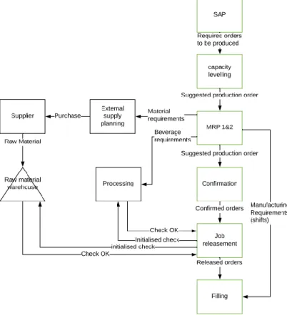
4.1 Supply chain
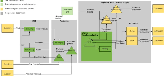
The company uses a make-to-stock policy to provide goods to its customers. The company’s supply chain in Sweden is illustrated with the high level flow chart, provided in Figure 6 below. The colour coding explained in Figure 6 illustrate which department is responsible for each operation.
Figure 6: The company’s supply chain in Sweden
Starting from the suppliers at the left side of Figure 6, the raw material is received at the processing facility. Packaging materials such as glass bottles and labels are received at the warehouse facility. These raw materials are purchased from a multitude of suppliers, from Sweden, Europe and other parts of the world. After the beverage is produced it is sent to be tapped and packaged in an operation called packaging, in which there are several different productions lines.
From the packaging department pallets are sent to the finished goods warehouse where the majority of the stock is kept. Apart from this main warehouse at the production site, the company also rent warehousing space and services from a third-party logistics service provider, when the capacity of the main warehouse is insufficient. Most of sales need to be shipped from the company’s warehouse, and stock moved to external warehouses most often need to be brought back to the main warehouse before being shipped. At the X-docs, see Figure 6, goods are consolidated for transports to its end customers.
24
If SKUs are needed at a certain time when it cannot be produced because of limitations and complexity in the production, SKUs and liquids can be sourced from other manufacturing units.
4.2 Processing
This section presents the relevant aspects of the operations under the department responsible for producing the beverage.
The beverage is produced using raw material delivered to the incoming warehouse and then stored in pressurised bulk tanks. Various production constraints for various products should be considered in this step. For some articles, extra constraints exist for the size of the batch due to raw material packaging that must be consumed immediately after it is opened. In this instance the batch size must correspond to a multiple of raw material packages. For other articles, constraints exist for the size of the batch due to the tank sizes. There is a minimal production volume affiliated with all products.
4.3 Packaging
The products are packaged at the packing lines in the manufacturing unit. The packaging facility contains seven packaging lines which use several types of bottles and cans in different volumes and with different production rates.
The packaging lines are open for production in accordance to the shift applied to that line, see Table 1. The time that employees are present at the lines is called the lines “opening hours”. This should not to be confused with the production hours of the line, which is the time of actual production. Other activities that are done during the opening hours are cleaning, training of personnel and maintenance. Table 1 shows the opening hours for each of the shifts used.
Table 1: Opening hours in production during a week.
The first activity at the line is to fill a package with its product. After that the packages are consolidated into larger selling units called pieces. The last activity at the line is to put the pieces on a pallet. The activity with the lowest throughput, the “bottleneck” of the machine, is the actual filling of the package.
All products manufactured by the company is associated to a specific “recipe group”. A recipe group is a range of products, defined by the company that shares the same
characteristics. Each recipe group, and consequently all products included in it, can only be packaged on one line.
Shifts Hours 1-shift 40 2-shift 76 3-shift 114 4-shift 138 5-shift 168
25
4.3.1 Production Fulfilment
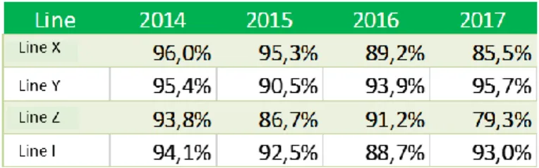
The production fulfilment of the packaging lines states how much of the planned volume per week that was produced. The planned amount is the amount set for production the Sunday before the production week, which is measured against the actual output the Sunday at the end of the week. This amount can vary greatly, and the resulting volume for a week can both be higher and lower compared to the planned volume. Reasons for lower output than
planned include machine breakdowns, issues that result in a lower production speed or a problem in material supply. Reasonings for a higher than planned output most notably includes a higher production speed than planned for and consequently an increase from the plan for lines starving for capacity. This puts extra strain on suppliers and purchasing department to make sure there are material in stock in case of extra production.
As can be seen in Table 2 below, the mean of the production fulfilment is generally below 100%. A production fulfilment below 100% signifies a yield loss, while a production fulfilment of above 100% signifies a yield gain. Later in the report both shall be named yield loss, where a negative yield loss signifies a yield gain.
Table 2: Average production fulfillment during the last 4 years for the four studied production lines.
4.3.2 Changeover Process
The company use several production lines to produce their SKUs. Since the number of production lines are considerably less than the number of SKUs, and the machine need to be adjusted for different kind of SKUs, all lines are subject to changeovers.
The changeover requires different operations depending on which combination of SKUs is in succession of each other, signifying that the time for changeover is sequence dependent. For example, a change from a 12-pack to a 6-pack of the same beverage is fast while a change from a fruity beverage to a clear carbonated water will require additional operations.
The characteristics of the changeover, and the times and costs associated with it, vary from line and type of product. For weeks close to current time, where the production sequencing is known, a matrix is used to determine the planned changeover time in the production. For long-term planning, the sequencing is not known, and estimation must be used.
Two different definitions of the changeover time in the production exist in the company. The packaging operations define the changeover as tap-to-tap. This means the time from where the last package was filled of the old batch to the time where the first package is filled from the new batch. The planning department on the other hand define the changeover time as what is referred to as pallet-to-pallet. This is the time from where the last full pallet was
26
retrieved of the old batch by the forklifts to the time where the first full pallet of the new batch is retrieved.
The taping is the bottleneck on all lines in the packaging department.
Each changeover carries a cost of cleaning materials and a start-up waste in beverage. The time spent on changeover is also costing the company employee-time not spent producing. The lines are subject to fixed costs of depreciation, maintenance, utilities etc. The time spent doing changeover also result in more volume that need to be sourced, inducing more costs. Since determining these costs have not been a goal of the thesis, and the gathering of this data have been deemed to extensive for this project, these costs will be taken at face-value from the production controllers of the company.
Three different suggestions to approximate the changeover cost have been considered. First, all changeovers taking place on a line could be said to carry the same cost. Secondly,
approximating on a recipe group level results in that only similar products carrying the same changeover cost. Lastly, an estimation on a SKU level could be done, resulting in all SKUs having their individual changeover cost. The chosen approach for this thesis is the recipe group level and the reasoning for this will be explained in chapter 5.
After the packaging operation is done and the pallets of produced SKUs are finished they are picked up by LGVs (Laser Guided Vehicles) and transported to the warehouse.
4.3.3 Line Efficiency
One of the major KPIs the packaging department is measured on is their output compared to the maximul theoretical output of the machines. One-hundred percent efficiency is defined as the line running full speed all the available time (opening hours), i.e., the entire time
operators are scheduled to work. The efficiency is then the ratio of actual time run with the actual speed and the available time there are operators available running on maximum speed.
In a perfect world the difference from the actual efficiency and the maximum efficiency would be due only to change-over downtimes. However, the lines do not always run on maximum capacity when online, and they are subject to breakdowns and other stops reducing
efficiency further.
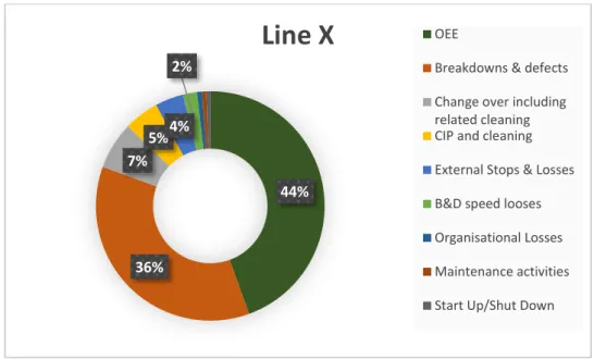
Figure 7 below shows an example of how the opening hours is allocated on one of the lines. OEE (Overall Equipment Effectiveness) is the fraction of time the machine is running on full speed.
27
Figure 7: Activity distribution for the open time of line X.
The relationship between changeover time and efficiency is clear, the efficiency loss is simply the changeover time divided by the total time. The relationship between breakdown and efficiency is also clear, breakdown results in an efficiency of zero for the disrupted time. The deviation from maximum line speed when it is running can be explained by several different factors. These include different mechanical problems, retrieval problems in the warehouse and ramp-up issues.
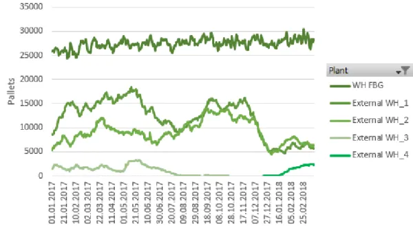
4.4 Warehouse
The company uses several warehouse facilities. Beside the main warehouse, the company have throughout 2017 rented spaces in four external warehouses. The inventories are transported between the locations by an external truck company. When the company ship inventory between the warehouses, they have the option to purchase a transport with goods one way (single transportation) or transportation of goods back and forth to a warehouse (double transportation). There is no special dedication of the articles to specific locations in the warehouses.
It is the planning department that decides what to transport between the warehouses and when. The decision is then communicated to the warehouse department which handles the administrative process of booking transportations and preparation of goods to be
transported. The planning department receive a suggestion from SAP of what goods that should be transported and when, although what the planner chose to ship often deviate from SAP’s suggestion.
How the finished goods are distributed among the warehouse is presented in figure 8 below.
44% 36% 7% 5%4% 2%
Line X
OEEBreakdowns & defects Change over including related cleaning CIP and cleaning External Stops & Losses B&D speed looses Organisational Losses Maintenance activities Start Up/Shut Down
28
Figure 8 stock on hand at the warehouses dated back to January 1, 2017.
Figure 8 illustrate that the external warehouses are always used. The number of stored pallets at the external warehouses are varying throughout of the year while the main
warehouse inventory are kept at around 27 000 pallets which corresponds to a utilization of 75%. This utilization is expressed as a target utilization in the main warehouse. The
variations of inventory levels are an effect of seasonality and variations in demand which will be more thoroughly explained in the analysis.
4.5 Information systems
The company utilize several different IT systems to align and streamline daily operations and strategic decisions. This chapter will provide a brief overview of these systems.
4.5.1 SAP
SAP is the ERP (enterprise resource planning) system used by the company. It integrates and consolidates information form the whole enterprise, serving as the working platform for several functions of the company. This report will mainly focus on SAP functions tied to the planning of production and warehousing operations.
4.5.2 Production follow-up tool
As a graphical feedback tool from the production, the company uses a self-developed software. From this application the user can quickly and easily get a good grasp of how the production is performing. The information in the follow-up tool is available for all departments.
4.5.3 MES
The company’s manufacturing execution system (MES), serves as the interface between the rest of the information architecture and the production floor. The MES measures, controls
29
and serves as the interactive software for the operators to enter or retrieve information to SAP.
The MES collect real-time data and transfer it both to the production follow-up tool and SAP, allowing the planning department to act in time to avoid or lessen the consequence of complications.
4.5.4 Warehouse Management System (WMS)
While SAP keep track of the high-level inventory management, the WMS have low level, more exact, information of the flow in the warehouse. As an example, SAP only have information of which SKUs that are kept in a warehouse and in which quantities, while the WMS can point to the exact location in the warehouse. The WMS is also used for planning and keeping track of ingoing and outgoing shipments
4.5.5 Business Intelligence software (BI)
The company uses a business intelligence service to retrieve data from SAP in manageable report formats which can also be converted to excel format. The service is flexible, and users have the ability to create new reports by using preset templates which can then be shared with other employees, creating a standardized report format which can be used for analysis. As all the systems are connected to SAP, and the BI retrieves and presents the data from SAP, the BI can present data originating from the MES or WMS. This gives full insight in these systems from the BI.
4.6 Inventory Control
This section presents the relevant aspect of how the company is controlling their inventory and how their results are measured.
4.6.1 Batch Size
Currently the company does not use any theoretical model to determine the batch size in their production. SAP uses a batch quantity when scheduling the production that is based on either a fix quantity or the demand of a set number of weeks. These amounts are set when the product is accepted in the portfolio based on similar products and is iteratively updated if major failures are recognized.
4.6.2 Service Level
When a new customer order is received, the stock is immediately checked to verify that the full volume of the order can be satisfied from stock on the specified shipping date. The volume that is accepted is classified as ATP (Available to promise) and is confirmed to the customer. The fraction of the volume that cannot be satisfied from stock is classified as PO2-volume and is rejected. HL is an abbreviation for hectolitres.