2005:27 DECOVALEX III/BENCHPAR PROJECTS Approaches to Upscaling Thermal-Hydro- Mechanical Processes in a Fractured Rock Mass and its Significance for Large-Scale Repository Performance Assessment

SKI Report 2005:27

Research

DECOVALEX III/BENCHPAR PROJECTS

Approaches to Upscaling

Thermal-Hydro-Mechanical Processes in a Fractured Rock

Mass and its Significance for Large-Scale

Repository Performance Assessment

Summary of Findings

Report of BMT2/WP3

Compiled by:

Johan Andersson

Isabelle Staub

Les Knight

February 2005

SKI Report 2005:27

Research

DECOVALEX III/BENCHPAR PROJECTS

Approaches to Upscaling

Thermal-Hydro-Mechanical Processes in a Fractured Rock

Mass and its Significance for Large-Scale

Repository Performance Assessment

Summary of Findings

Report of BMT2/WP3

¹JA Streamflow AB, Älvsjö, Sweden

²Golder Associates AB, Stockholm, Sweden ³Nirex UK Ltd, Oxon, United Kingdom February 2005

This report concerns a study which has been conducted for the DECOVALEX III/ BENCHPAR Projects. The conclusions and viewpoints presented in the report are those of the author/authors and do not

Foreword

DECOVALEX is an international consortium of governmental agencies associated with the disposal of high-level nuclear waste in a number of countries. The

consortium’s mission is the DEvelopment of COupled models and their VALidation against EXperiments. Hence theacronym/name DECOVALEX. Currently, agencies from Canada, Finland, France, Germany, Japan, Spain, Switzerland, Sweden, United Kingdom, and the United States are in DECOVALEX. Emplacement of nuclear waste in a repository in geologic media causes a number of physical processes to be

intensified in the surrounding rock mass due to the decay heat from the waste. The four main processes of concern are thermal, hydrological, mechanical and chemical.

Interactions or coupling between these heat-driven processes must be taken into account in modeling the performance of the repository for such modeling to be meaningful and reliable.

The first DECOVALEX project, begun in 1992 and completed in 1996 was aimed at modeling benchmark problems and validation by laboratory experiments.

DECOVALEX II, started in 1996, built on the experience gained in DECOVALEX I by modeling larger tests conducted in the field. DECOVALEX III, started in 1999

following the completion of DECOVALEX II, is organized around four tasks. The FEBEX (Full-scale Engineered Barriers EXperiment) in situ experiment being

conducted at the Grimsel site in Switzerland is to be simulated and analyzed in Task 1. Task 2, centered around the Drift Scale Test (DST) at Yucca Mountain in Nevada, USA, has several sub-tasks (Task 2A, Task 2B, Task 2C and Task 2D) to investigate a number of the coupled processes in the DST. Task 3 studies three benchmark problems: a) the effects of thermal-hydrologic-mechanical (THM) coupling on the performance of the near-field of a nuclear waste repository (BMT1); b) the effect of upscaling THM processes on the results of performance assessment (BMT2); and c) the effect of glaciation on rock mass behavior (BMT3). Task 4 is on the direct application of THM coupled process modeling in the performance assessment of nuclear waste repositories in geologic media.

On September 25, 2000 the European Commission (EC) signed a contract of FIKW-CT2000-00066 "BENCHPAR" project with a group of European members of the DECOVALEX III project. The BENCHPAR project stands for ´Benchmark Tests and Guidance on Coupled Processes for Performance Assessment of Nuclear Waste Repositories´ and is aimed at improving the understanding to the impact of the thermo-hydro-mechanical (THM) coupled processes on the radioactive waste repository performance and safety assessment. The project has eight principal contractors, all members of the DECOVALEX III project, and four assistant contractors from

universities and research organisations.The project is designed to advance the state-of-the-art via five Work Packages (WP). In WP 1 is establishing a technical auditing methodology for overseeing the modeling work. WP´s 2-4 are identical with the three bench-mark tests (BMT1 - BMT3) in DECOVALEX III project. A guidance document outlining how to include the THM processes in performance assessment (PA) studies will be developed in WP 5 that explains the issues and the technical methodology, presents the three demonstration PA modeling studies, and provides guidance for inclusion of the THM components in PA modeling.

This report is the final report of the BMT2 of DECOVALEX III and its counterparts in BENCHPAR, WP2, with studies performed for establishing approaches for upscaling the hydro-mechanical properties of the fractured rocks and their impacts on far-field performance of potential radioactive waste repositories.

L. Jing F. Kautsky J.-C. Mayor O. Stephansson C.-F. Tsang January 2005 Stockholm, Sweden

Summary

The Benchmark Test 2 of DECOVALEX III and Work Package 3 of BENCHPAR concerns the upscaling THM processes in a fractured rock mass and its significance for large-scale repository performance assessment. The work is primarily concerned with the extent to which various thermo-hydro-mechanical couplings in a fractured rock mass adjacent to a repository are significant in terms of solute transport typically calculated in large-scale repository performance assessments. Since the presence of even quite small fractures may control the hydraulic, mechanical and coupled hydro-mechanical behaviour of the rock mass, a key of the work has been to explore the extent to which these can be upscaled and represented by ‘equivalent’ continuum properties appropriate PA calculations. From these general aims the BMT was set-up as a numerical study of a large scale reference problem. Analysing this reference problem should:

‰ help explore how different means of simplifying the geometrical detail of a site,

with its implications on model parameters, (“upscaling”) impacts model predictions of relevance to repository performance,

‰ explore to what extent the THM-coupling needs to be considered in relation to

PA-measures,

‰ compare the uncertainties in upscaling (both to uncertainty on how to upscale or

uncertainty that arises due to the upscaling processes) and consideration of THM couplings with the inherrent uncertainty and spatial variability of the site

specific data.

Furthermore, it has been an essential component of the work that individual teams not only produce numerical results but are forced to make their own judgements and to provide the proper justification for their conclusions based on their analysis. It should also be understood that conclusions drawn will partly be specific to the problem analysed, in particular as it mainly concerns a 2D application. This means that specific conclusions may have limited applicability to real problems in 3D. Still the

methodology used and developed within the BMT should be useful for analysing yet more complicated problems.

Several conclusions can be drawn from the individual team analyses as well as from the interaction discussions held during Workshops and Task Force meetings:

‰ Interpretation of given data constitutes a major source of uncertainty. During the

course of the project it was certainly felt that these interpretation uncertainties could have a large impact on the overall modelling uncertainty.

‰ Differences between teams in estimated effective permeability appear to depend

essentially on whether the team used given apertures as input - and then calculated fracture transmissivity using the cubic law – or if the hydraulic test data were used to calibrate the fracture transmissivity distribution. Furthermore, the assumptions used as regards fracture size versus aperture (or permeability) are not fully proven. Different assumptions on this would, although not really tested in the Task, lead to large differences in upscaled properties.

‰ The calculated effective rock mass deformation modulus differs between teams

but all teams include the “given” value of the test case. It appears that this problem is relatively “well behaved”.

‰ If modelling uses relaxed initial apertures as input the HM coupling is essential

for capturing realistic permeabilities at depth. However, this does not necessarily imply that the HM couplings need to be considered. The fact that the aperture versus stress relation reaches a threshold value indicates that the more normal practice of fitting hydraulic properties to results of hydraulic tests is warranted! A key process, where there still is uncertainty is the relation between hydraulic residual aperture and maximum mechanical aperture, Rb. Evidently this has a strong influence on the impact of the HM coupling. Related to this is the indication found on the significance of the increase of differential stress results in increasing the permeability (when applying the non-linear stiffness model for fractures) and in channelling of flow path (potentially caused by fracture

dilation).

Despite the relatively limited amount of large scale analyses conducted within the Task, some general remarks seem possible. It is suggested the stress is so high at the depth of the repository that fractures are almost completely compressed mechanically and the permeability is approaching its residual value. Therefore further stress increase due to thermal stresses would not significantly reduce the permeability. Also the TH effects, due to buoyancy, are relatively limited and would add an uncertainty in the order of a factor of 2 or so.

These observations support the conclusion that it is the uspcaling of hydraulic

properties rather than the added complication of T and M couplings, which are the main sources of uncertainty in a problem of this nature. The added disturbance, in relation to in-site stress, is small in the far-field of a deep repository. Yet, understanding the

stress/permeability relation is important for understanding the nature of the permeability field.

It can also be noted that most conclusions to be drawn from the large scale analyses could already be drawn from studying the intermediate performance measures such as permeability, deformation modulus and k versus stress relations.

Sammanfattning

Denna rapport sammanfattar resultaten från beräkningsfallet BMT2 inom projektet DECOVALEX III (motsvarar WP3 inom projektet BENCHPAR). Inom detta

beräkningsfall analyseras i vilken utsträckning olika termo-hydro-mekaniska (THM) kopplade processer har betydelse for masstransporten i större skala från ett slutförvar i sprickigt berg.

Eftersom även små sprickor kan tänkas påverka grundvattenströmning och

bergmekanik har arbetet fokuserat på hur inverkan av små sprickor kan ”skalas upp” till ekvivalenta egenskaper för bergmassan. Beräkningsfallet har därför lagts upp som en numerisk studie av ett referensproblem. Studien har haft följande mål:

‰ undersöka hur olika sätt att förenkla den geometriska detaljerna i

bergbeskrivningen ”uppskalning” inverkar på modellprediktioner av betydelse för funktionen hos ett geologiskt djupförvar

‰ undersöka i vilken utsträckning, i relation tilll förvarsfunktionen,

THM-kopplingar därvid behöver tas med

‰ jämföra osäkerheterna i uppskalningen och THM-processerna med den

ofrånkomliga osäkerheten och rumsliga variationen i platsdata.

En viktig del av arbetet har dessutom varit att de olika deltagande grupperna inte bara genomför numeriska beräkningar, men tvingats göra egna bedömningar och underbygga slutsatserna från deras analyser.

Flera olika slutsatser kan dras från arbetet:

‰ Tolkning av data utgör en stor källa till osäkerhet.

‰ Skillnaden mellan olika gruppers uppskattade effektiva permeabilitet verkar bero

på om man använt (uppskattade) sprickaperturer eller resultatet av faktiska hydrauliska tester som indata.

‰ Relationen mellan spänning och sprickapertur är osäker – och har stor betydelse

för resultatet av kopplade beräkningar. En tillhörande fråga är den

aperturförändring som uppstår vid skjuvdeformationer. Denna kan vara klart större en påverkan från normalspänningen och kan dessutom ge permanenta effekter.

‰ Om beräkningarna utgår från obelastade sprickaperturer är det synnerligen

väsentligt att ta hänsyn till den hydromekaniska kopplingen för att beskriva permeabilitet och grundvattenströmning på stort djup. Men det betyder inte att denna koppling måste tas med vid all modellering. Om beräkningarna istället baseras på faktiska uppmätta hydrauliska egenskaper vid aktuella djup har denna koppling redan tagits om hand i fältdata. Då är kopplade beräkningar inte

nödvändiga. För det aktuella fallet gäller speciellt att spänningarna på djupet är så höga att sprickaperturerna redan nått sitt residualvärde. Ytterligare

spänningsökningar kommer därvid inte att påverka permeabiliteten nämnvärt.

‰ Uppskattad effektiv elasticitetsmodul för bergmassan varierar mellan grupperna,

men inom ett begränsat intervall.

De gjorda observationerna ger därvid stöd till slutsatsen att det är uppskalningen av de hydrauliska egenskaperna, snarare än T och M kopplingen, som är den dominerande osäkerheten i denna typ av problem. Störningen från ett förvar är begränsad i

fjärrområdet. Det hindrar inte att relationen mellan spänning och permeabilitet är viktig för att förstå karaktären av permeabilitetsfältet.

Contents

1.1 Objectives and setup pf the task 1

1.2 Participating teams 2

2 The reference problem 3

2.1 Problem to be analysed 3

2.2 Input data 3

2.3 Performance measures 7

3 Approaches to upscaling 9

3.1 Overall approach 9

3.2 Small scale analyses 9

3.3 Large scale analyses 11

4 Upscaling from detailed data into effective parameters 13

4.1 Fracture statistics 13

4.2 Hydraulic upscaling 21

4.3 Mechanical upscaling 26

4.4 Hydro-mechanical analyses 27

5 Large scale analysis 32

5.1 Impact of heat source on T, H and M properties 32

5.2 Particle tracking – the overall performance measures 36

5.3 Discussion 39

6 Conclusions 41

6.1 Interpretation of the discrete fracture network data 41

6.2 Effective permeability 41

6.3 Upscaling the mechanics 42

6.4 Need for coupled analyses in the far-field? 42

References 43

1 Introduction

This report concerns the upscaling of thermo-hydro-mechanical (THM) processes in a fractured rock mass and its significance for large-scale repository performance

assessment as studied in the BMT2 Test Case in the international DECOVALEX III project and in WP3 of the EU-funded BENCHPAR project. Different research teams have conducted the work and the details of analysis are reported separately by each team. This report focuses on the lessons learnt.

1.1 Objectives and setup of the task

BMT2 of DECOVALEX and WP3 of BENCHPAR are primarily concerned with the extent to which various thermo-hydro-mechanical couplings in a fractured rock mass adjacent to a repository are significant in terms of radionuclide solute transport typically calculated in large-scale repository performance assessments (PA). Since the presence of even quite small fractures may control the hydraulic, mechanical and coupled hydro-mechanical behaviour of the rock mass, a key aspect of the work has been to explore the extent to which these can be upscaled and represented by ‘equivalent’ continuum

properties appropriate for PA calculations.

It must be understood that this task, even when simplified to two dimensions, is both intellectually and mathematically extremely challenging and at the limit of current computer hardware and software capability. For this reason the objectives have not been framed in absolutist terms of ‘how to upscale’ but rather to investigate how the

uncertainties inherent in the upscaling process impact on the derived PA-relevant parameters.

Given this, the task has two, closely integrated aims:

To understand how an explicit acknowledgement of the need for upscaling of coupled processes alters the approach to performance assessment modelling and the analysis of the model results;

To understand the uncertainty and bias inherent in the outputs from performance assessment models in which the upscaling of THM parameters is either implicit or explicit.

From these general aims the task was set-up as a numerical study of a realistic large-scale reference problem, see Chapter 2 below. Analysing this reference problem should:

help explore how different means of simplifying the geometrical detail of a site, with its implications on model parameters, (“upscaling”) impacts model predictions of relevance to repository performance.

explore to what extent the THM-coupling needs to be considered in relation to PA-measures.

compare the uncertainties in upscaling (both to uncertainty on how to upscale and uncertainty that arises due to the upscaling processes) and consideration of THM couplings with the inherrent uncertainty and spatial variability of the site specific data.

Furthermore, it has been an essential component of the work that individual teams not only produce numerical results but are forced to make their own judgements and to provide the proper justification for their conclusions based on their analysis.

Finally it should be understood that conclusions drawn will partly be specific to the problem analysed, in particular as it mainly concerns a 2D application. This means that specific conclusions may have limited applicability to other problems in 3D. Still the methodology used and developed within the Task should be useful for analysing yet more complicated problems.

1.2 Participating

teams

In total eight different teams analysed the Task either as part of DECOVALEX III (five teams) or as parts of BENCHPAR (three teams). Table 1-1 provides the name of the teams as well as full reference to the individual team report.

Table 1-1. Teams and references to the team reports

Team Acronym used in this report

Part of Reference to team report

INERIS/ANDRA,

France Ineris BENCHPAR Progress report 1

st _{of April 2002}

Final report .1st _{of October 2003}

Kyoto University/ JNC, Japan

JNC DECOVALEX Kobayashi et al. (2003)

KTH/SKI, Sweden KTH BENCHPAR Last provided progress report (January 2003)

DOE/LBNL,

U.S.A. LBNL DECOVALEX First draft final report from DOE/LBNL, June 2002 AECL/OPG,

Canada OPG DECOVALEX Draft final report prepared by AECL for OPG (Chan et al. October 2003), Guvanasen and Chan (2004)

Uppsala

University/STUK, Finland

STUK DECOVALEX Last progress report (may 2003), some data from PR 5.5.2001

Univ. of

Birmingham/Nirex UK

UoB/NIREX DECOVALEX Progress Report 2002, Draft version 2.0

PhD thesis (October 2003) (Blum, 2003)

UPV/ENRESA, Spain

UPV BENCHPAR Gómez-Hernández, and Cassiraga

2

The Reference Problem

The problem addressed concerns a hypothetical heat producing repository placed at depth in a hypothetical fractured rock. However, in order to get realistically complex and spatially varying geologic data, the hydrogeologic and hydromechanical input data were loosely based on the basement geology around Sellafield, United Kingdom, and on the site characterisation data acquired by Nirex. However, it must be emphasized that the geometry analysed is purely fictional and does not represent the actual conditions at Sellafield.

A key characteristic of the rock mass considered is that the fracture density and fracture size both show fractal behaviour. This is not unusual for such rock types, but implies that there may not be a scale at which equivalent continuum behaviour exists. Further, it might be predicted a priori that spatial scales at which continuum behaviour is shown might differ for thermal, mechanical and hydrological properties, as for many individual couples.

2.1 Problem to be analysed

The reference problem concerns the far-field groundwater flow and solute transport for a situation where a heat producing repository is placed in a fractured rock medium. Radionuclides potentially released from the repository may migrate with the

groundwater flow and thus reach the biosphere. Specific issues at stake are:

how to assess the far-field hydraulic and transport properties when most data stem from small scale (borehole) tests,

what is the impact of potential mechanical and hydraulic couplings, and if MH or HM couplings are significant how would they affect the upscaling? The reference problem geometry is shown in Figure 2-1. It is assumed that the HLW (heat source) is encased within resaturated bentonite within a repository drift shown as a simple horizontal body. (NB no attempt is made to represent repository detail such as deposition holes etc.). The repository sits within a low permeability fractured rock unit which is overlain by a second low permeability fractured rock unit that extends to ground surface. A vertical fracture zone cuts both rock units but lies beyond the end of the repository tunnel.

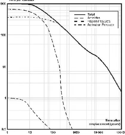
The repository is assumed to comprise of 60 uniformly distributed canisters of HLW embedded in compacted and resaturated bentonite, with a canister density of 6·10-3

canisters/m2 (or 60 canisters per 100 m x 100 m). Figure 2-2 shows the heat evolution versus time for each canister.

2.2 Input

Data

The relevant data for the rock formations and fault are based on Sellafield site characterisation data acquired by Nirex. The data are in the form of statistical

distributions of properties. Typically, most of the data concern measurements on a small scale, whereas the problem to be studied mainly concerns the large scale.

Not to Scale 5 km 1km Detailed model area Formation type 1 Formation type 2 Repository block 5m 100m 10m 100m 50m 500m Vertical fault zone 100m Sea

Figure 2-1: Reference problem geometry

2.2.1 Fracture

statistics

2.2.1.1 Fracture orientation

The orientation data were extracted from Nirex (1997a). The orientation data and the dispersion are set-dependent and are presented for the two formations and the fault zone in

Table 2-1, Table 2-2 and Table 2-3, respectively.

2.2.1.2 Fracture lengths

Fracture length data was obtained from analysis of 1-dimensional scan-line data at outcrop, 2-dimensional outcrop trace maps and 2-dimensional aerial photography lineaments [Nirex 1997e, page 46]. Combined data sets obtained from the above sources, for all fracture orientations, show a power law distribution of fracture (trace) lengths such that the number of fractures per km2 of length greater than L(m) is given by:

D

CL

N ₌ − _(2.1)

where N is the number of fracture (traces) per km2 of length L(m), C= 4 106 and D=2.2 [+/- 0.2] [for a 2-dimensional fracture network], respectively.

Figure 2-2: Heat source – each canister

Table 2-1. Fracture orientation for Formation 1

Mean dip (º) Dip direction (º) Fisher Kw

Set 1 08 145 5.9

Set 2 88 148 9

Set 3 76 021 10

Set 4 69 087 10

Table 2-2. Fracture orientation for Formation 2

Mean dip (º) Dip direction (º) Fisher Kw

Set 1 25 028 7.2

Set 2 81 156 9.4

Set 3 72 020 11

Set 4 68 090 8.1

Table 2-3. Fracture orientation for the Fault Zone

Mean dip (º) Dip direction (º) Fisher Kw

Set 1 08 021 6.8

Set 2 76 150 11

Set 3 72 021 13

These data sets did not include fractures of very small trace length. For consistency it is recommended that the above relationship should not be extrapolated to fractures with trace lengths less than 0.5 m.

2.2.1.3 Fracture frequency and fracture density

Linear fracture frequency is expressed by means of mean and maximal vertical spacing for each fracture set in each Formation (Table 2-4, Table 2-5 and Table 2-6) [Nirex, 1997a]. The spacing is obtained from measurements done in vertical and inclined boreholes and that have been corrected using a Terzaghi correction to estimate true spacings measured perpendicular to the fracture sets.

Table 2-4. Vertical spacing data for Formation 1

Max spacing vertical (m) Mean spacing vertical (m)

Set 1 5.35 0.29

Set 2 2.21 0.26

Set 3 2.01 0.28

Set 4 3.54 0.31

Table 2-5. Vertical spacing data for Formation 2

Max spacing vertical (m) Mean spacing vertical (m)

Set 1 4.29 0.51

Set 2 2.5 0.35

Set 3 3.83 0.28

Set 4 2.26 0.41

Table 2-6. Vertical spacing data for the Fault Zone

Max spacing vertical (m) Mean spacing vertical (m)

Set 1 1.43 0.18

Set 2 1.41 0.18

Set 3 1.06 0.19

Set 4 1.32 0.22

Fracture density has been shown to be a function of sampling technique, in particular the lower cut-off in the smallest fracture size included in the fracture sample is directly related to fracture density. Compilation of outcrop, borehole, aerial photography and structural maps suggests that the relationship for 2-dimensional surfaces is of the form [Nirex 1997f]:

1

( ) 2.4 E( 2.4 / )

density m− _{= ⋅}x− ₌ x _(2-2)

where x is the cut off (m) and E is a power law exponent = 1.

A 2-dimensional fracture density can be derived for any specified fracture cut-off length. The same relationship should be taken as representative of both Formations and the Fault Zone. As noted in the previous section it is recommended that a lower cut-off in fracture length used in modelling should be set at 0.5 m.

2.3 Performance

measures

The study concerns the impact on calculated performance of coupled processes and associated upscaling strategies – not what is a ‘strictly correct’ means of upscaling. The significance of different assumptions and methods used in the upscaling should thus be compared through specified measures relevant to the performance being explored (far-field flow and solute migration). Furthermore, some intermediate measures, i.e. resulting upscaled parameter values are worthwhile to comparing.

2.3.1 Overall

performance

measures

Ultimately, the performance measure for a repository PA would be doses or risk, however, in order not to introduce too many assumptions about the waste, release mechanisms or the retention properties of different solute species the general performance measures studied here were restricted to the groundwater specific contribution to retention. The research teams were thus asked to predict performance measures using the following strategy.

In several different publications Cvetkociv et al. (1999) showed that the breakthrough along a single streamline essentially depends upon two different parameters:

1 ( )v s ds

τ =

_∫

2

1 ( ( ) ( ))v s b s ds 1Q s ds( )

β =

_∫

_∫

where v(s) is the fluid velocity along the streamline, b(s) the fracture aperture and Q2(s)

(m2/s) the specific flow rate. (The total flow rate in fracture Q is given by ∫Q2(w)dw

integrated perpendicular to the streamlines in the fracture). Interpretation of the

parameters in equations (2-3) and (2-4) are that the τ is the transit time (distribution) for a particle(s) in the flowing water and β describes the retardation capacity of the rock matrix. The parameter β is called the “transport resistance”.

In practice it turns out that β is by far the most important parameter of the two since it relates to the possibilities for interaction between the flowing water and the rock matrix. In the safety assessments carried out in Sweden and Finland, it is this retention

(diffusion into the matrix combined with sorption inside the matrix), which has effect on reducing releases. It can be shown that β is equal to the product awtw used to in the

far-field migration code used in SKB SR 97 (SKB, 1999), WL/Q used in safety

assessments in Finland (see e.g. Vieno and Nordman, 1999) or arL/q used in SKI

SITE-94 (SKI, 1996).

Consequently teams were asked to provide both “transit time (τ) distributions” and "transport resistance (β) distributions" at two output surfaces:

a perimeter surface at 50m outwards from the boundary (wall/floor/roof) of the repository.

2.3.2 Intermediate

performance

measures

It turns out that most upscaling techniques lead to the formulation of effective permeability, effective rock mass deformation modulus or effective porosity to be used in large scale numerical models. Consequently, it is usually possible to directly compare two different upscaling approaches by comparing the resulting effective parameters. In fact, during the course of work, such intermediate parameters comparisons have been a more practical, and quicker tool, than the ultimate comparison of the overall

3 Approaches

to

upscaling

This chapter discusses the different approaches to upscaling and subsequent problem analysis used by the different teams.

3.1 Overall

approach

At a simplistic level the analysis may be considered to comprise a number of steps: 1. Analyse the rock mass fracture, hydraulic, thermal and mechanical, data provided by

Nirex and abstract appropriate parameters. Derive appropriate conceptual and mathematical models.

2. Derive a description at the small scale using discrete fracture network approaches (2D or 3D) or by continuum analyses.

3. Derive upscaled equivalent hydraulic, mechanical and coupled hydro-mechanical properties for the small scale description. This involves analysis at a range of scales to ensure that appropriate representative upscaled equivalent continuum parameters are derived (the REV). This is a non-trivial exercise since there is no guarantee that there is such a scale, it may vary between properties and existing software places limits on the number of fractures that can be considered so that some form of

simplification may be necessary. Clearly some uncertainty may be introduced in this step

4. Parameterise a large-scale continuum model with values obtained from step 3 and analyse the importance of the various couples in the rock mass surrounding a deep repository to determine their importance on solute transport properties at a PA scale. These steps are further outlined in the following sections.

3.2 Small scale analyses

In general the teams have applied three different approaches to analysing the small scale data: crack tensor theory, discrete fracture network simulations and continuum approaches.

3.2.1 Crack

tensor theory approach

Two teams (OPG and JNC) applied the crack tensor theory (Oda, 1986) for deriving effective permeability and rock mass mechanical properties, but the JNC team later discarded this approach.

The OPG approach was based on Oda’s Crack tensor theory, extended to include thermohydromechanical parameters (Guvanasen and Chan 2004). Two types of

aperture, mechanical and hydraulic, are used in the extended theory. Parameters based on the extended Crack Tensor Theory – bulk elastic properties, permeability, porosity are dependent on effective stress. The extended Crack Tensor Theory has been implemented in the FRACTUP code. An approximation of the FRACTUP upscaling

calculation has been incorporated into AECL’s MOTIF finite-element code for THM modelling.

3.2.2 Discrete

fracture network approaches

Several teams tried to describe the fractures statistically by a Discrete Fracture Network (DFN) model and then use the DFN-model as input to hydraulic and mechanical analyses to derive effective permeability and rock mass mechanical properties at different block sizes.

Ineris generated DFN simulations in 3D with the RESOBLOK computer code, and determined equivalent parameters in different size models. The 3D DFN models were used as input for H- and HM computations in 3DEC. Due to software and hardware limitations, upscaling was limited to at most 5 m cube scale, and most often only at 2 m cube scale, depending on the parameter. No REV could be reached.

JNC applied a numerical Pixel methods for the examination of the scale effect. JNC generated 3D fracture network in 60 m cube, and then extracted data for 2D fracture density, length and intensity on the model plane. A vertical 2D plane located at the centre of the model was defined and divided into 20 cm pixels. Sub-regions of different scales were randomly produced from this plane (from 5*5 to 30*30 m sizes), the size of the pixel was the same for all sub-regions. The pixel method is based on evaluation of hydraulic and mechanical processes on the 60 m plane and its sub-regions. The number of fractures existing in each pixel was counted and the permeability was assumed proportional to the number of fractures in each pixel. The model was calibrated by assigning permeability for each pixel in the different model sizes according to fracture information, and the effective permeability for the sub-regions at different scales was then calculated.

KTH generated fracture networks in 2D and the 2D models were then used as input to UDEC for hydraulic and mechanical calculations. The determination of

equivalent properties for a REV was based on stochastic realisations of the DFN at different scales (from 0.25 m to 10 m square). The DFN models were generated within 300*300 m boxes to avoid boundary effects.

STUK split the problem into a hydrological part (H) and a thermo-mechanical part (TM). The hydrological approach was based on 3D DFN models (FracMan-Mafic) with multiple stochastic realisations to determine the directional hydraulic

conductivity versus angle plots that allow examination of the validity of the

continuum approximation at a 7.5 m scale. Fracture transmissivity was derived from the hydraulic borehole data. Hydraulic aperture for fractures was calculated from the transmissivity by the cubic law, under an assumption of parallel plates. Particle tracking at the same scale was also performed using hydraulic apertures. M and TM analyses were performed with a separate large model using UDEC (2D) to explore the effect of excavation, backfilling and heating on fracture apertures at various locations and for different main fracture orientations. These results were transferred to the hydrological small scale model as a sensitivity study.

UoB/NIREX generated 2D fracture networks, with power-law fracture length distributions as input in UDEC for THM analysis. The limitations of UDEC in flow calculations and representativity of a DFN model greater than 10 m x 10 m were overcome by developing the fracture flow code FRAC2D. H analyses were

performed with constant hydraulic aperture in order to determine effective hydraulic permeability tensors. HM-analysis was performed by linking UDEC-BB with

FRAC2D and then estimating the modified effective permeability tensors. Some TM- and TH-analyses would be possible with UDEC and could be conducted on modified apertures due to thermal processes.

3.2.3 Continuum

approaches

Two teams applied continuum approaches:

LBNL applied an upscaling method based on a Heterogeneous Porous medium model and Fractal Levy-stable distribution at the 1.56 m scale chosen to make use of a series of short interval hydraulic tests. Upscaling was performed by numerical experiments and stochastic simulations. The stochastic simulations are based on a fractal Levy distribution for permeability at the support scale (1.56 m) up to the grid block scale (up to 50 m). A stress-permeability relationship was added to the

analysis. Particle tracking was conducted on each numerical gridblock in order to fit a gridblock scale dispersivity distribution.

UPV applied Laplacian upscaling to 50 m blocks for average flow reproduction. Upscaled K is the ratio of total flow to head gradient.

3.3 Large scale analyses

The general approach to the large scale analysis has been rather similar between the teams, although different software has been used. It appears that differences in results (see next chapter) depend generally on differences in input parameters rather than in different codes used.

The teams have used the following approaches:

Ineris compared T, TH, TM and THM computation using an equivalent medium code (FLAC3D). The equivalent properties derived from the upscaling.

JNC evaluated the large scale problem with scaling rules obtained from Crack Tensor theory, but used the mean values provided in the Task.

KTH applied the equivalent parameters from small scale analysis in THM coupled FEM code (ROCMAS) based on continuum media. At first stage non coupled hydraulic, mechanic and thermal analysis were done based on the protocol’s definition and parameters.

LBNL employed multiple realizations of subsurface heterogeneity to determine the mean flow and transport processes and the associated uncertainties. T2R3D (Wu et al., 1996) was used to simulated coupled TH and tracer transport processes - with and without heat. A sensitivity study on the influence of fracture porosity was conducted.

OPG incorporated an approximation of the FRACTUP upscaling algorithm developed for small-scale analysis into the THM simulator MOTIF. MOTIF was applied to examine the macro-scale impact of TH(HT) HM(MH) and THM processes on the migration of radionuclides. Three sets of large-scale simulations were undertaken:

1. Nirex rock mass parameters given in the Problem Definition and Description were directly input into MOTIF for H only, TH (HT), HM (MH) and THM analyses.

2. HM (MH) and THM simulations were performed with effective rock mass permeability, porosities and deformation moduli calculated at each time step for every element in the large-scale model. All fractures were considered to

contribute to the rock mass properties.

3. As in 2) above except that only 1/3 of all fractures were assumed to be active. STUK applied TOUGH2 to solve the head and flux field, with upscaled parameters of effective conductivity and correlation structures for the 7.5 m scale that are obtained from the DFN modelling. Transport was modelled by particle tracking, using the conductivity, head and flux fields from the hydraulic simulations and distributions of transit time and transport resistance at the 7.5 m scale from the DFN modelling. Multiple realisations, only concerning H and transport, have been

conducted but TM effects were studied as sensitivity analysis based on input permeability distributions.

UoB/NIREX: Upscaled HM-modified, effective hydraulic conductivity tensors (keff)

were evaluated at REV scale (10 m × 10 m), which could be used in the regional continuum model. The continuum flow and transport code FAT3D was used for the far-field studies.

UPV solved the full problem using a detailed description of the hydraulic conductivity field and by using an upscaled description. The results were then compared.

4

Upscaling from detailed data into

effective parameters

This chapter discusses the results from the upscaling of the detailed scale data into parameters amenable for large scale numerical analysis, i.e. into effective permeability and deformation (tensors).

4.1 Fracture statistics

Many upscaling approaches were built on the fracture statistics. However, as the fracture data were given as observations and not as prescribed fracture statistical distributions, different teams made different interpretations of the data.

4.1.1 Fracture

orientation

Fracture orientations were provided for each fracture set in the input data description and are presented in section 2.2.1. The way the different teams treated and applied the discontinuity orientations data is reviewed briefly below. The approaches are

summarised in Table 4-1.

Table 4-1. Approaches on fracture orientation

Team Source for orientation Application

Ineris Orientations as given in Task 3D generation (Resoblok) JNC Orientation as given in Task 3D generation

KTH Orientation as given in Task 2D DFN model

LBNL Not used -

OPG Orientation as given in Task 3D

STUK Orientation as given in Task 3D DFN generation (FracMan)

UoB/Nirex Orientation as given in Task 2D fracture generation (FracFrac) using a constant fracture set orientation

UPV Not used

INERIS: The fracture orientation was treated in 3D and the values are taken from the

protocol. Fisher dispersion was taken into account.

JNC: The fracture orientation was generated in 3D according to the orientation

distribution given in the Task input definition. 2D vertical planes were extracted from these 3D models for further analyses.

KTH: The KTH team generated the fractures in 3D on the basis of dip and dip direction of each fracture set as given in Table 2-1 to Table 2-3, and their Fisher coefficient. Then orientations of generated fractures were converted from 3D data into 2D using the following formula:

θ α

β tan cos

tan = (4-1) with β=Apparent dip angle, α=True dip angle, θ=Angle between the model plane

(159°/90°) and the dip direction of the fracture sets. All four sets were modelled in KTH team analysis since the density of all four fracture sets were considered to be the same.

OPG: The fracture orientation was treated in 3D using data given for all four fracture sets in the Task definition. Fisher dispersion was taken into account.

STUK: For hydraulic analyses the STUK team used the Task defined orientations (Table 2-1 to Table 2-3) in 3D and generated 3D DFN models. For the 2D mechanical analysis the 3D orientations of the 3 sets were rotated in the perpendicular direction to the model plane while the dip remained unchanged.

UoB/NIREX: The UoB/Nirex team transformed the 3D orientation data given in the Task definition into 2D by projecting the 3D mean dip angles onto the 2D-model plane adopted. The conversion was done using equation (4-1).

The statistics of transformed fracture orientation were then used to generate 2D DFN models. The 4th fracture set was neglected in the 2D models because it showed almost the same strike and dip as the model plane. Two options were developed in the Fracture Network Generator to account for dispersion of fracture orientation (expressed by the Fisher coefficient in Table 2-1 to Table 2-3): i) no account was made for dispersion and only the mean apparent dip angle was used for each fracture set; ii) dispersion was considered and the Fischer coefficients were used to generate the apparent dip angles for each fracture set.

The coefficients defined in Table 2-1, Table 2-2 and Table 2-3 illustrate a fairly high dispersion of fractures in each fracture set. Nevertheless visual comparisons of DFN generated with the Fisher distribution and the trace maps clearly indicate that a high dispersion of orientation does not produce synthetic networks that are comparable to those observed. It is apparent that fracture orientation dispersion is length dependent with low dispersion of longer fractures and higher dispersion of shorter fractures.

Remarks: Essentially, the teams have used the orientation distribution as given in the test case definition. However, there is room for interpretation on how to use these distributions, which are given in 3D, for the 2D applications followed by some teams.

4.1.2 Fracture

size

According to the Task input definition the fracture length distribution can be described by a Power Law function, see equation 2-1. Most of the teams used the equation with a transformation of length units, i.e.:

2 . 2 4 ) (_{L = L}− N (4-2) where N(L) is the cumulative number of fractures per m2 of length greater than L(m). The mean fracture length, µL, derived from this equation is expressed as:

min 1 L D L D µ = − (4-3)

where Lmin is the cut-off min applied for the fracture length distribution. The way the

different teams interpreted and applied the fracture length distribution law is briefly described below and the approaches are summarized in Table 4-2.

Table 4-2. Approaches on fracture size estimation

Team Distribution C D Cut-off length min Cut-off lengt h max Mean trace length Comment

Task data Power law 4 2.2 0.5 -

Ineris Power law 4 D1=1.2

D2=0.7 D3=1.1 D4=1.1 0.5 - - D values for each set, formation 1 JNC Power law 4 2.2 0.5 250 m 0.92 KTH Power law 4 2.2 0.5 250 m 0.92 2D

OPG Power law 4 2.2 0.5 -

STUK, all

fractures Power law 4 3 0.5 >200 - 2D cut-off, 3D D parameter STUK,

conductive fractures

Power law 4 3 0.83 >200 - 2D cut-off, 3D D parameter UoB/Nirex Power law 4 2.2 0.5 0.92 Task data, 2D

(Max)

3.23 2.08 0.5 0.96 Mean

1.2 2.2 0.5 0.92 Low

LBNL Not used - - - -

STUK: The 3D fracture length distribution used by the STUK team is based on the 2D power law relationship that uses an exponent and a cut-off radius (equation 4-2). The 3D fractal exponent D was simply extrapolated by adding 1 to the fractal dimension of the 2D length distribution given in the Task problem definition. The fractal exponent D is given to be 2.2 [±0.2]. However, because of software limitations the Power Law exponent was stated as 3. The off diameter in 3D was extrapolated from the 2D cut-off trace length by a factor 1.6. The cut-cut-off radius was then half the cut cut-off diameter extrapolated from the given value in the Task problem definition.

Considering all fractures (conductive and non conductive), min off and max cut-off length of 0.5 and 250 m were used, which means that the equivalent 3D min radius cut-off is 0.4 m (=0.25*1.6).

From an ‘OSNES analysis’ the proportion of conductive fractures was estimated to be 40% of all fractures. The removed non-conductive fractures are predominantly short fractures and the adjustment of the fracture length distribution for conductive fractures was made by increasing the cut-off radius in the model. The new cut-off can be

calculated from the primitive of equation 4-2 expressed as:

1.2

4 ( )

1.2

N L = − ⋅L− (4-4)

By considering the standard cut-off values, N(L) was expressed by (N(250)-N(0.5)) distribution. Taking away 60% of the non-conductive fractures towards the small fractures N(L) was expressed as 0.6*(N(250)-N(Lmin,cond)) distribution. By

combining this expression to equation 4-4 the 2D length cut-off is 0.83 m. The fracture trace length distribution was then based on equation 4-2, but using a min length cut-off of 0.83 m and a max length cut-off of 250 m. The corresponding 3D min radius cut-off being used was 0.65 m, while the maximum radius was never used, since the side length of the cubic DFN realizations was only 20 m.

KTH: The 2D fracture trace length distribution used by the KTH team is based on the Power-law distribution (equation 4-2) with fractal coefficient D of 2.2 and constant C of 4 as given in the Task definition. A max and min length cut-off of 0.5m and 250m were used for the generation of the size distribution. Fracture length was generated in the model from the inverse form of the cumulative distribution function derived from equation 4-2 and the expression is:

(

)

(

)

2.2 2.2 2.2 2.2

min min max

L= cut− −F cut− −cut− − (4-5)

where L is the fracture length and F is a random number.

The mean trace length was calculated on the basis of equation 4-3 and is 0.92m.

INERIS: The Ineris team used the fracture size distribution defined by a Power law function (equation 4-2). A min cut off of 0.5 m is used. The coefficient C is 4 as defined in the Task. The fractal dimension D was specified for each fracture set. D for sets 2, 3 and 4 were based on information given in the Task and extracted from Nirex, 1997e. D for set 1 of all formations was estimated (no values are provided). Fracture networks with threshold length at 0.25, 0.5 and 1 m were also generated for sensitivity analyses.

UoB/NIREX: In its first evaluation the UoB/Nirex team used the Power-law function as defined in the Task (equation 4-2) with C=4, D=2.2. Based on equation 4-3,

µL=0.92m. The Power law parameters provided are defined on a combination of data

sets. However the further investigations showed that these mean data are only appropriate if the data set of the trace map is not considered. The team decided to conduct sensitivity analysis on C and D that can be inferred from the data sets, and that give low, middle and upper values for the function parameters, and as such new

equations for fracture length and values for the mean fracture length: lower case: n(L)=1.2⋅L-2.2_{; µ} L=0.92m mean case: n(L)=3.23⋅L-2.08_{; µ} L=0.96m higher case: n(L)=4⋅L-2.2_{; µ} L=0.92m

The fractures were generated in the 2D DFN models according to these Power Law equations, and two options were available: 1) cut-off min (0.5 m) and no cut-off max; 2) cut-off min (0.5 m) and cut-off max (250 m).

JNC: The JNC team used a fracture length distribution based on the power law function (equation 4-2). The length of fractures was truncated at 0.5 m and 250 m. The mean fracture length was calculated from equation 4-3 and is 0.92 m. The length of fractures was generated from the following equation:

( )

(

)

OPG: OPG obtained a 2D surficial fracture trace length distribution using the BMT2-defined power law with exponent equal to 2.2 and a cutoff length of 0.5 m. The 2D fracture length distribution (chord of a circular disc) was translated into diameter distribution for respective circular fractures.

In summary, and as is evident from Table 4-2 the given data could lend itself to different interpretations. To some extent, but not only, this is due to whether the

subsequent analysis was made in 2D or 3D. Of particular interest are assumptions made on correlation between size and hydraulic properties as (at least implicitly) assumed by e.g. the STUK team. Clearly, the Task input data set was ambiguous with regard to this – and the resulting differences in interpretation may be seen as a reflection of this uncertainty.

4.1.3 Fracture

density and intensity

There are various ways of describing fracture density or fracture intensity. A useful notation1 was introduced by Dershowitz (1985) and later developed in the manual to the DFN-code FracMan (e.g. Dershowitz et al., 1995):

P10= number of fractures per length (number of fractures/m), (“fracture frequency”),

also called P11 by INERIS.

P20=number of fractures per area, (number of fractures /m2),

P21=total trace length per area, (m/m2), also P22 (INERIS)

P30=number of fractures per volume (number of fractures /m3), (“fracture density”),

equivalent to P31 defined by INERIS.

P32=total fracture surface per volume (m2/m3) (“fracture intensity”)

Evidently, P10, P20 and P21 all depend on the direction of the observation line or plane

(and of the fracture orientation distribution). Furthermore, Dershowitz (1985) shows that there is a linear relation between e.g. P10 and P21 and between P21 and P32, whereas

the relation between P30 (“fracture density”) and P10 (“fracture frequency”) strongly

depends on the fracture size distribution.

The fracture frequency in 2D (P20, number of fractures/m2) can be calculated from

equation 4-2 and taking into account the cut-off min and cut-off max. The following expression is then used:

(

)

estimation of the number of fractures of all sets.

The fracture density in 2D, P21, can be derived from this expression:

20

21 P

P =µ_L (4-8) with µL mean fracture length as defined in equation 4-3. The approach undertaken by

the different teams is presented below and the summary is illustrated in Table 4-2

INERIS: The Ineris team obtained the linear fracture frequency P10 (P11 in the Ineris

team notation) from vertical borehole analysis extrapolated from diagrams provided in the Task specification The min cut-off is 0.5 m. P10 for all fracture sets in formation 1 is

1.97 m-1. The linear fracture frequency was also estimated (from the same aforementioned figure) for models generated with threshold at 0.25 and 1 m.

1 _{The FracMan modelling team has unfortunately not been fully consistent in their use of this notation. In}

P21 (called P22 by the team) was obtained from measurements on horizontal 2D map

analysis and estimated from equation 2-2 for Lmin=0.5m to: P21,m=5 m/m2.

The input required in the 3D fracture generator is the 3D fracture frequency, P30

(called P31 by the team). The value of P30 was chosen by calibration on simulation

results in order to fit the measured values of P10 and the estimated value of P21. For the

first run the value of P30 has been set equal to P10 (P30=2 /m3). Then sampling on several

horizontal cross-sections was done to check the correspondence of the simulated P30 to

P21. The back-calculated values from simulations of P21 and P30 were consistent with

measured data of P21. P21 was estimated from simulations to 4.39 and 5.01 m/m2 for

cubes of respectively 3 and 4m side sizes, and P32 to 4.74-5.39 m2/m3 for the same cube

sizes. The fracture intensity P32 was determined from the RESOBLOCK simulations.

KTH: The team calculated the fracture frequency in 2D, P20, on the basis of equation

4-7. The resulting P20 was18.38 fractures/m2 applying Lmin=0.5 m and Lmax=250 m.

Assuming an equal frequency of fractures in each fracture set P20 per fracture set is

equal to 4.6 fractures/m2. The team used the same equation (4-8) to calculate the 1D fracture frequency and the 2D fracture density. P21=P10= P20*µL = 16.91 m-1. The value

of P10 can be compared to the estimated value from the vertical mean spacing (given in

the protocol), P10=14.1/m for formation 1.

STUK: The input parameter required by FracMan is P32, which is unknown but can

be calibrated against mean vertical spacing using to the following expression:

10 3 3 32 C P S C P _p f p = (4-9)

Using the mean vertical spacing values listed in Task protocol P32 was calibrated with

Cp3 of 0.843 with an r2 value of 0.999. P32 is defined for each fracture set by best fit

estimation from several realisations of the 3D fracture model, and by sampling: 1) perpendicular mean fracture spacing, 2) 2D fracture intensity (sampling on horizontal trace planes) and 3) mean vertical spacing. The references are P21=4.8 m-1, P10=5.53

fractures/m and mean vertical spacing as given in the protocol. P21 is the mean value

estimated from equation 2-2 for a min cut-off of 0.5 m. P10 is the vertical fracture

frequency for all sets in one formation.

The fracture intensity P32 for conductive fractures was estimated by reducing the P32

for all fractures by the amount of non-conductive fractures according to the following relationship.

10 32 21 10 32 21

2.25 5.53

cond cond cond

P P P

P = = P = P (4-10)

UPV: Fracture information was used to define the ranges of the variograms used to generated the spatial distribution of heterogeneous conductivities. After several tests and the recommendation by the steering committee hydraulic conductivities were generated using a variogram with vertical anisotropy and ranges of 20 m in the vertical direction and 10 m in the horizontal.

UoB/Nirex: The fracture density in 2D, P21, was estimated using two approaches.

In the first approach the fracture density was derived from the Power Law distribution by applying equations 4-7 and 4-8, and using a min cut-off of 0.5 m and a max cut-off of 250 m. As mentioned in section 4.1.2 three sensitivity cases were considered that

define low, medium and high density cases.Different values of P20 and P21 were then

calculated for the three different cases:

lower case: For C=1.2 and D=2.2, P20=5.51 m-2, P21=5.05 m-1

mean case: For C=3.23 and D=2.08, P20=13.66 m-2, P21=13.15 m-1

higher case: For C=4 and D=2.2, P20=18.38 m-2, P21=16.91 m-1

The fracture density was estimated from equation 2-2. Applying a lower cut-off of 0.5 m, the fracture density P21 is 4.8 m-1 with a maximum of 10 m-1 and a minimum of

around 2 m-1. The three cases illustrate the sensitivity of fracture data analysis to the choice of the Power Law length distribution. The fracture density calculated for the lower case, P21=5.05 m-1, is close to the mean measured and given fracture density

(extrapolated from a figure given in the Task definition), P21=4.8 m-1. The mean vertical

fracture spacing was calculated for each formation and compared to the measured mean vertical spacing data provided in the Task protocol. The mean vertical spacing was estimated from vertical boreholes data adjusted according to a Terzaghi correction. The data were analysed statistically and the best-fit PDF was achieved by an exponential distribution.

The second approach used the data provided in the protocol for mean vertical spacing and transformed these by projecting the 3D fracture spacing onto the project plane using the following equation:

β α α cos cos t S S = (4-11) with St mean true spacing (m), Sa mean apparent spacing, β apparent dip angle and α true dip angle. The apparent mean spacing was used for weighting the density of fractures in each set when using the calculated P20 as input for generation of fractures.

JNC: The 2D fracture frequency P20 was calculated using equation 4-7, applying a

min cut-off of 0.5 m and a max. cut-off of 250m. P20=18.4 fractures/m2 for all sets. The

2D fracture density, P21, was derived from equation 2-2. Applying this equation and

using a min cut-off of 0.5 m this leads to P21=4.8 m-1. This value was compared to the

value calculated based on the Power Law distribution of fracture length, equation 4-8. Using a min cut-off of 0.5 m and a max cut-off of 250 m the calculated P21 for all sets

then is 16.9 m-1. Since the discrepancy in P21 was considered as an uncertainty for

fracture information both definitions are examined and their influence on upscaling results considered.

OPG: OPG determined P30 and P32 by analyzing the given surficial data to obtain the

distribution of fracture diameter and density.

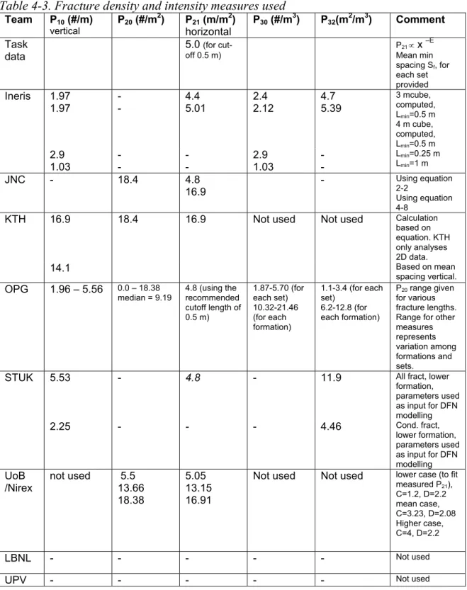
Table 4-3 summarizes values of fracture density estimated by different teams.

4.1.4 Spatial distribution, termination and shape of fractures

The various assumptions made on the spatial distribution of fractures can be summarised as follows:

JNC: The JNC team distributed the centre of fractures randomly in the 3D model and the fractures were assumed to be circles.

Table 4-3. Fracture density and intensity measures used Team P10 (#/m) vertical P20 (#/m2) P21 (m/m2) horizontal P30 (#/m 3_{) P} 32(m2/m3) Comment Task data 5.0 (for cut-off 0.5 m) P21 ∝ x –E Mean min spacing Sf, for each set provided Ineris 1.97 1.97 - - 4.4 5.01 2.4 2.12 4.7 5.39 3 mcube, computed, Lmin=0.5 m 4 m cube, computed, Lmin=0.5 m 2.9 1.03 - - - - 2.9 1.03 - - Lmin=0.25 m Lmin=1 m JNC - 18.4 4.8 16.9 - Using equation 2-2 Using equation 4-8

16.9 18.4 16.9 Not used Not used Calculation based on equation. KTH only analyses 2D data. KTH 14.1 Based on mean spacing vertical. OPG 1.96 – 5.56 0.0 – 18.38

median = 9.19 4.8 (using the recommended cutoff length of 0.5 m) 1.87-5.70 (for each set) 10.32-21.46 (for each formation) 1.1-3.4 (for each set) 6.2-12.8 (for each formation) P20 range given for various fracture lengths. Range for other measures represents variation among formations and sets.

STUK 5.53 - 4.8 - 11.9 All fract, lower

formation, parameters used as input for DFN modelling 2.25 - - - 4.46 Cond. fract, lower formation, parameters used as input for DFN modelling UoB /Nirex not used 5.5 13.66 18.38 5.05 13.15 16.91

Not used Not used lower case (to fit measured P21), C=1.2, D=2.2 mean case, C=3.23, D=2.08 Higher case, C=4, D=2.2 LBNL - - - Not used

UPV - - - Not used

STUK: The STUK team assumed circular disk fractures. The STUK team also

considered the data on fracture termination. The data on fracture terminations were used for the spatial generation of the 3D DFN model. 27% of the fractures were generated from uniformly located fracture centres, while the remaining 73% were generated from locations uniformly distributed on surfaces on existing fractures.

KTH: For the KTH team no spatial distribution was assigned for the generation of fractures in space so fractures are randomly distributed in the model.

INERIS: The Ineris team considered the fractures as polygons. Fracture density P30 (P31 in INERIS notation) is assumed to follow a Poisson law;

UoB/NIREX: The UoB/Nirex team generated fractures following a Poisson distribution. A development of the algorithm for generating midpoints of fractures by the repulsion method has been completed (Chillingworth, 2002). However, the repulsion algorithm was not used in the task.

OPG: The OPG team represented fractures by circular disks. Only disks with centroids located within the averaging volume were used.

Remarks: The spatial model chosen for the generation of fractures might have a significant influence on the calculation and simulation of effective hydraulic conductivity. Again, there are differences between teams, which originate from assumptions (necessary) rather than from hard data.

4.2 Hydraulic

upscaling

The approach to hydraulic upscaling differs between teams using DFN-analyses and the teams using a porous medium approach only. The latter only considers the hydraulic measurements in the different scales, whereas the former combines the model of the fracture network with the hydraulic information for the upscaling.

4.2.1 DFN and Crack Tensor Theory approaches

Various approaches to upscaling into effective permeability based on DFN-modelling or other discrete techniques have been applied by the teams. These are outlined below:

JNC: JNC used a pixel method for upscaling hydraulic properties and conducted a sensitivity study on the influence of fracturing. The pixel method, applied in 2D, was based on 3D DFN realisations generated according to fracture information in 150 m cubes. The reference plane for the pixel method was chosen as the centre vertical section. This original plane was divided by pixels of 0.2 m square. The hydraulic conductivity of each pixel is proportional to the number of fractures counted in this pixel and related to the average measured logarithm of permeability and its standard deviation. The scale effect was studied in sub-regions from 5 m*5 m up 60 m *60 m size, representing the finite element mesh on the original plane divided into pixels of equal dimension. The vertical and horizontal 1D flow was examined in each sub-region by applying a hydraulic gradient equivalent to the length of the sub-region. The

equivalent permeability of a sub-region was obtained as an average velocity at the outlet boundary based on unit hydraulic gradient and identical element size. The scale effect was studied by the variation of the average and standard deviation of homogenized permeability for different size sub-region. The average homogenized permeability slightly increases with scale while the standard deviation decreases much with scale. The permeability calculated for each sub-region could be identified as the effective parameter if its value coincides with the geometric mean. Tests conducted on the 5 and 30 m sub-regions showed that this approximation might be true.

Sensitivity to upscaling was tested by dividing the large region (60 m x 60 m) in sub-regions and trying to estimate the effective permeability of the large region consisting of sub-regions. Each sub-region has an effective permeability value given from the pixel method described above. The same hydraulic boundary conditions were set to the sides

of the large region model. The results show that the geometric mean has a good

agreement with the effective hydraulic conductivity especially for sizes greater than 5m. Since the geometric mean coincides with the effective hydraulic conductivity the

lognormal distribution can be appropriate for the hydraulic conductivity distribution in sub-regions.

KTH: The KTH team analysis was based on multiple stochastic realisations of 2D DFN model. For each realisation in a 300*300 m2 square, scale models ranging from 0.25 to 10 m are extracted and for each model the directional permeability was calculated by applying specific pressure boundary conditions in UDEC. Constant hydraulic aperture for zero normal stress was calculated as arithmetic mean of the data from the four tested cores, and set to 65 µm. The investigations on the applicability of continuum approach was also studied by rotating each DFN model stepwise 30° and comparing the result with the one predicted by second order permeability tensor transformation. The evaluation of directional permeability was based on the extended Darcy’s law for anisotropic homogeneous media. The simulations showed that the directional permeability decreases as the model size increases but becomes constant beyond a certain size, which indicates the existence of a REV. The presence of the equivalent permeability tensor (and so the existence of a REV) was demonstrated if the calculated directional permeability values and the average permeability tensor conform to an ellipse. Based on results of previous simulations an equivalent permeability tensor was reached when the model size was equal to or greater than 5m, and a REV can be given with acceptable variation and prediction error.

INERIS: The hydraulic analyses of the Ineris team are based on DFN models and 3DEC simulations. 3 different boundary conditions are applied in 3DEC to determine the equivalent permeability tensor. The analyses were based on 5 stochastic realisations of DFN models at each model size (from 2 to 5 m). For each model size, the equivalent vectorial flow rate was averaged from the flow rate value at different locations of the fracture network after each computation at different boundary conditions. A constant hydraulic aperture was assumed. However, computer limitations made most of the realisations at 3 and 4 m scale impossible to evaluate. The permeability tensors calculated at three model sizes (2, 3 and 4 m) showed that the values change with size but remain in the same order of magnitude. Running more models at bigger scale than 2 m are required to be able to determine the REV and check whether the components of the permeability tensor come to an asymptotic level. Also the impact of artificial joint prolongations and fracture length threshold was investigated. The prolongation of joint up to the next block face (that artificially increased the fracture network connectivity) could lead to overestimate the permeability by a factor of 2 or 3. Increasing the fracture threshold length seems to increase the permeability, whereas the number of fractures in the model decreases. The problem might be related to independent simulations of fracture network for the different tests, and the minimum fracture length approaching the size of the model.

OPG: The OPG team developed a permeability field by applying Guvanasen and Chan’s (2004) modification of Oda’s crack tensor theory. The test scale was a 100 m x 100 m model. Input data include the rock matrix elastic constants and fracture set geometric and mechanical data. Mean data provided in the Task are used for the rock matrix mechanical properties. Distributions of fracture geometry properties given in the Task definition are used whenever available. The Cumulative Distribution Function for hydraulic aperture was estimated from the BMT2-given transmissivity distribution (inferred by Nirex from short-interval hydraulic pulse tests). The interpretation of the tests was made assuming that all fractures within a single test interval have the same