2004:14 Modelling of Radionuclide Transport by Groundwater Motion in Fractured Bedrock for Performance Assessment Purposes

SKI Report 2004:14

Research

Modelling of Radionuclide Transport by

Groundwater Motion in Fractured Bedrock

for Performance Assessment Purposes

Anders Wörman

Joel Geier

Shulan Xu

October 2003

SKI perspective

Background

The Swedish site investigation programme is ongoing and is rapidly producing site specific data that will be included in SKB’s site descriptive models, preliminary safety evaluations and in the final safety assessments SR-Can and SR-Site. To be prepared for the review of these reports, SKI will need to perform some independent modelling as regards groundwater flow and radionuclide transport, using a selection of the available site specific data.

The purpose of this study is to develop a performance assessment (PA) model for analyses of radionuclide transport in the geosphere that accounts for the effect of heterogeneities of hydrological as well as geochemical rock properties. This is

accomplished by coupling of sub-models for water flow (the discrete-fracture network model developed for SKI by Joel Geier, Geier 2004) and solute transport (developed by Xu et al, 2001 and Wörman et al., 2003). Moreover, measured geochemical data from Äspö Hard Rock Laboratory in Sweden is used to exemplify how the discrete-fracture and the solute transport models are coupled. The coupled model also enables an assessment of whether a process, that is important in the small scale (time or space), is important also on the larger geosphere scale.

Relevance for SKI

The work presented in this report is a step forward in developing a coupled groundwater flow and radionuclide transport model and as such is an important part of SKI’s work in PA modelling.

The proposed approach includes numerical simulations of the three-dimensional fluid flow in a discrete feature network and a one-dimensional analytical solution of

heterogeneous (random) mass transfer through the series of fractures. This method leads to a mathematically simple coupling of the solute transport with the three-dimensional flow problem as well as rapid computations that are suitable for future risk assessments and performance assessments.

Results

This study has successfully coupled a three-dimensional flow model and a

one-dimensional mass transfer model, thereby creating an integrated model suitable for risk assessments and performance assessments.

Preliminary analyses performed with this integrated model indicate that regional/global variability in flow velocity and fracture aperture dominates over the local-scale

variability as regards the effect on solute transport. However, site-specific data on both a fracture (local) scale and regional scale is required to reach a definite conclusion regarding the relative importance of local- and regional-scale variability.

It is also shown that the effect of heterogeneous rock properties on radionuclide

transport in rock fractures increases markedly with decreasing fracture aperture and the co-varying advection velocity. It is concluded that the effect of variability in bedrock properties on the larger network-scale may be much larger that on the local scale. This may have a great importance for implementation in for instance risk assessments.

Future work

Future activities will be to take this work forward within the framework of the SKI performance assessment group that meets regularly two times per year to discuss ideas and present results from various projects dealing with issues relevant for PA modelling.

Project information

SKI project manager: Eva Simic

SKI Report 2004:14

Research

Modelling of Radionuclide Transport by

Groundwater Motion in Fractured Bedrock

for Performance Assessment Purposes

Anders Wörman¹

Joel Geier²

Shulan Xu³

¹Department of Biometry and Engineering

Swedish University of Agricultural Sciences

Box 7013

SE-750 07 Uppsala, Sweden

²Clearwater Hardrock Consulting

14505 Corvallis Rd

Monmouth

OREGON 97361-9603, USA

³Swedish Radiation Protection Authority, SSI

SE-171 16 Stockholm

October 2003

This report concerns a study which has been conducted for the Swedish Nuclear Power Inspectorate (SKI). The conclusions

Contents

Summary...3

Sammanfattning ...5

1. Introduction ...7

2. Theoretical background...11

2.1 3-D flow and travel time description of solute transport ...11

2.2 Theory for one-dimensional solute transport...13

2.3 Deterministic analysis of solute transport with spatially variable rock properties...16

2.4 Evaluation of Covariance Structures of Transport Properties of Crystalline Rock and Implications to Solution Procedure ...18

2.5 Methodology of solving one-dimensional stochastic solute transport problem.21 2.6 Extending the solutions to a network scale ...25

2.7 One-Dimensional Continuum Model ...27

3. Illustrative application based on a discrete-feature model...29

3.1 Discrete-feature model for water flow analysis ...29

3.2 Simulations of hydrological properties of discrete-fracture network ...31

3.3 Extraction of parameters for one-dimensional solute transport...36

3.4 A comparison of the travel time approach and the one-dimensional continuum model ...38

4. Determination of longitudinal dispersion coefficient on a fracture scale ...41

4.1 Theoretical background ...41

4.2 Empirical relationship between dispersivity and Peclet number...44

5. Discussion of model behaviour based on site specific data... 46

5.1 Uncertainty due to spatial variability of mass transfer...46

5.2 Combination of flow effects and uncertainty of spatial variability of mass transfer ...52

6. Conclusions...54

7. References ...56

Appendix 1: Derivation of cross co-variance function ...60

Appendix 3: Derivation of Auto-covariance of Auxiliary Variable β(p; s) in

Summary

Field data of physical properties in heterogeneous crystalline bedrock, like fracture zones, fracture connectivity, matrix porosity and fracture aperture, is associated with uncertainty that can have a significant impact on the analysis of solute transport in fractured rock. The purpose of this study is to develop a performance assessment (PA) model for analyses of radionuclide transport in the geosphere, in which the model takes into account both the effect of heterogeneities of hydrological and geochemical rock properties.

By using a travel time description of radionuclide transport in rock fractures, we decompose the transport problem into a one-dimensional mass transfer problem along a distribution of transport pathways and a multi-dimensional flow problem in the fractured bedrock. The hydraulic/flow problem is solved based on a statistical discrete-fracture model (DFM) that represents the network of fractures around the repository and in the surrounding geosphere. A Monte Carlo technique reflects the fact that the representation of the fracture network is uncertain.

If the flow residence time PDF exhibits multiple peaks or in another way shows a more erratic hydraulic response on the network scale, the three-dimensional travel time approach is superior to a one-dimensional transport modeling. Examples taken from SITE 94, a study performed by the Swedish Nuclear Power Inspectorate, showed that such cases can be found in safety assessments based on site data.

The solute transport is formulated based on partial, differential equations and perturbations (random spatial variability in bedrock properties) are introduced in the coefficients to reflect an uncertainty of the exact appearance of the bedrock associated with the discrete data collection. The combined approach for water flow and solute transport, thereby, recognises an uncertainty in our knowledge in both 1) bedrock properties along individual pathways and 2) the distribution of pathways.

Solutions to the central temporal moments of the residence time probability density function (PDF) for solutes in both one and three dimensions are derived in closed form for a solute Dirac pulse. The solutions are based on a model that takes into account advection along the network of fracture planes, diffusion into the rock matrix and sorption kinetics in the rock matrix. The most relevant rock properties including fracture aperture and several matrix properties as well as flow velocity are assumed to be spatially random along transport pathways.

The auto-covariance function representing the spatial variability in a rock property is also separated in terms of local variations, within individual fractures, and regional/global variations in a network of fractures. Analyses indicate that the regional/global variation probably dominates over the local variation due to the longer correlation lengths. This may have implications for planning of data collection, in which it is likely that one should pay more attention to the large-scale variations in bedrock properties. However, site-specific data (e.g. on the variance) is needed also on the single fracture-scale to be able to draw general conclusion on this issue.

Furthermore, measured geochemical data from Äspö Hard Rock Laboratory in Sweden is used to exemplify how the discrete-fracture and the solute transport models are coupled. Experimental studies based on rock samples taken at Äspö Hard Rock

Laboratory, reveal that crystalline bedrock can possess a marked heterogeneity of various physical and geochemical properties even on a fracture-scale. By inserting measurement values in the solutions we can conclude that the heterogeneity of the rock properties in single fractures contributes to increasing significantly both the variance and the skewness of the residence time probability density function for a pulse travelling in a fracture. The Äspö-data suggests that the bias introduced in the variance of the expected value of the residence time PDF for radionuclides by neglecting the heterogeneity of the rock properties is very large for fractures thinner than a few tenths of a millimetre. This bias would be even larger if the large-scale variation in bedrock properties on the network-scale was also accounted for.

Sammanfattning

Fältdata över fysikaliska storheter i heterogent kristallint berg, som sprickzoner,

spricknätverkan, matrisporositet, och sprickaperturer, uppvisar stora osäkerheter vilka kan ha en väsentlig betydelse för analyser av radionuklidtransport i sprickigt berg. Syftet med projektet som beskrivs i denna rapport var att utveckla en modell över radionuklidtransport i sprickigt berg som tar hänsyn till effekterna av heterogenitet i hydrologiska och

geokemiska egenskaper i berget. Modellen skall även vara användbar i säkerhetsanalyser över slutförvaret av radioaktivt avfall med hänsyn till beräkningstid och dataunderlag.

Genom att utgå från en beskrivning av uppehållstider (residenstider) för vattnets tredimensionella rörelse längs olika flödesbanor, kan ämnestransporten analyseras i en dimension längs dessa banor. Även om flödesberäkningen kräver komplicerade och arbetskrävande numeriska operationer ger denna metod väsentliga arbetsbesparingar både i beräkningsarbetet och i hantering av data. Lösningen till flödesproblemet baseras på en statistisk representation av diskreta (enskild) sprickor i ett nätverk kring slutförvaret och i den omgivande geosfären. Monte Carlo (statistiska) dator simuleringar reflekterar det faktum att de hydrologiska parametrarna är osäkra.

Om residenstidsfördelningen för flödet uppvisar flera toppar, på grund av flera dominerande flödesvägar i nätverket av sprickor, så är den tredimensionella (uppehållstids-) beskrivningen väsentligt bättre än en endimensionell modellering. Eventuella brister i modellbeskrivningen gäller både koncentrationstoppar och varaktigheten i ett

spridningsförlopp. Exempel som utvecklats från underlag i SITE 94, undersökningen som genomfördes av Statens kärnkraftsinspektion, visar att det mycket väl kan förekomma sådana flera flödesvägar i säkerhetsanalyser tillämpade på det svenska urberget.

Den lösta ämnestransporten formuleras med hjälp av partiella differentialekvationer. Perturbationer (statistiska störningar) införs i koefficienterna för att representera

osäkerheterna den rumsliga variationen i bergets egenskaper som uppkommer på grund av den punktvisa datainsamlingen. Det kombinerade angreppssättet för flöde och löst

ämnestransport tar därmed hänsyn till vår bristande kunskap om både 1) berggrundens egenskaper längs enskilda transportvägar och 2) fördelningen av transportvägar.

I rapporten härleds lösningar i sluten form till de centrala temporala momenten av täthetsfunktionen för uppehållstiderna för lösta ämnen i både en och tre dimensioner. Lösningarna tar hänsyn till advektion längs nätverket av sprickplan, diffusion och

sorptionskinetik i bergmatrisen. De flesta relevanta storheterna, inklusive sprickapertur, en rad storheter för bergmatrisen samt flödeshastigheten antas vara rumsligt slumpmässiga längs transportbanorna.

Auto-kovariansfunktionen, som representerar den rumsliga variabiliteten i bergets egenskaper, är separerad i form av en lokal variation, inom enskilda sprickor, och en regional/global variation i spricknätverket. Analyser indikerar att den regionala

(storskaliga) variationen förmodligen dominerar lösningen över de lokala variationerna på grund av längre korrelationslängder. Detta kan ha betydelse för planering av provtagningar genom att det förmodligen är viktigare att kunna beskriva de storskaliga variationerna i bergets egenskaper. Dock är det viktigt att ha platsspecifika data (t.ex. över varians) för att kunna dra definitiva slutsatser kring denna fråga.

Dessutom används geokemiska data från Äspö berglaboratorium för att exemplifiera hur den diskreta nätverksmodellen och modellen över den lösta ämnestransporten kan kopplas. Experimentella undersökningar baserat på prover från Äspö berglaboratorium visar att kristallint berg kan ha markanta variationer i olika fysikaliska och geokemiska egenskaper till och med i enskilda sprickor. Genom att sätta in mätvärden i de analytiska lösningarna kan man konstatera att heterogeniteterna i bergets egenskaper i enskilda sprickor bidrar väsentligt till att öka både varians och skevhet i uppehållstidsfördelningen för en ämnespuls i sprickan. Äspödatat indikerar att felet som uppkommer i variansen i den väntevärdesbildade uppehållstidsfördelningen för radionuklider genom att försumma heterogenitet i bergets egenskaper är mycket stort för sprickor som är tunnare än några tiondels millimeter. Felet skulle bli ännu större om man även tog hänsyn till de mer storskaliga variationerna i berget.

1. Introduction

Performance assessment of the Swedish final disposal for spent nuclear fuel involves modelling of possible leakage of radionuclides from a damaged canister in the deep bedrock repository. One of the important issues for the performance assessment is how data uncertainty and uncertainty due to spatial variability in rock properties can be addressed in the modelling and data acquisition.

Transport of solutes in fractured rock is affected by advection in conducting fractures and matrix diffusion as well as sorption onto the solid matrix. Various models have been developed to describe solute transport in fractures subjected to matrix diffusion and sorption (e.g. Neretnieks 1980, Grisak and Pickens, 1980 and Wels et al. 1994).

Most models describing radionuclide transport in fractured bedrocks do not include the effect of heterogeneity in rock properties and sorption kinetics on solute mass transfer. However, the impact of aperture heterogeneity in an individual fracture on solute transport has been described numerically using particle-tracking simulations (e.g. Moreno et al., 1988). Cvetkovic et al. (1999) analysed the effect of heterogeneous aperture and matrix diffusion on solute transport in a single fracture in terms of two spatially random parameters using a Monte Carlo technique. Recently, Painter and Cvetkovic (2001) extended their analysis of heterogeneous aperture and matrix diffusion to solute transport on a fracture network scale but without account taken to the effect of aperture

heterogeneity on the flow distribution.

The purpose of this study is to develop a performance assessment (PA) model for analyses of radionuclide transport in the geosphere, in which the model takes into account both the effect of heterogeneous rock properties on mass transfer and aperture

heterogeneity on the flow distribution. An alternative to achieve this objective is to use Monte Carlo simulations based on 3-D models that account for both hydraulics and solute mass transfer. However, such an approach would need unrealistically long computing time and this prohibits systematic investigations. A particularly fast method is required if the transport model is included in a risk framework with a large sequence or tree structure of models representing an entire pathway from the fuel rods to individual humans and possible evolution scenarios.

By using a travel time description of radionuclide transport in rock fractures, we decompose the transport problem into a one-dimensional mass transfer problem and a multi-dimensional flow problem. The proposed approach includes numerical simulations of the three dimensional fluid flow in a discrete feature network and a one-dimensional analytical solution of heterogeneous (random) mass transfer through the series of fractures. Hence, the de-coupling significantly reduces computational requirements both because the randomness of the flow and the solute transport are decoupled and because the solute transport is one-dimensional. The latter simplification implies important possibilities to solve the solute mass transport in certain closed-forms that will be discussed in this report. Furthermore, this method leads to a mathematically simple coupling of the solute transport with the three-dimensional flow problem and rapid computations that are suitable for future risk or performance assessments.

The hydraulic/flow problem is solved based on a statistical discrete-fracture network model that represents the system of fractures around the repository. This sub-model is described in more detail in another SKI-report (Geier, 2003) and will not be described in full detail here. The main purpose of this report is to demonstrate how the sub-models for water flow and solute transport are coupled and, particularly, to give examples on the use of field data in site specific investigations. A particular focus is on the stochastic solution techniques applied to the solute transport. Further, measured field data from Äspö Hard Rock Laboratory is used to exemplify how the discrete-fracture and the solute transport models are coupled.

A main problem is how to account for heterogeneity in rock properties. Recent experimental studies reveal that crystalline bedrock can possess a marked heterogeneity of various physical and geochemical properties (Hakami and Barton, 1990; Siitari-Kauppi et al., 1997; Xu and Wörman, 1998; Johansson, 2000) that potentially may have a certain impact on the transport of radionuclides in fractured bedrock. In addition, current field investigation techniques provide only fragmentary information of the properties of the geosphere. This is a basic motivation for treating flows of water and solute elements in groundwaters by means of stochastic models (Gelhar et al. 1974; Dagan, 1989; Gutjahr et al. 1978; Gelhar and Axness, 1983). The macro-dispersion in fractured bedrock has been studied, particularly using stochastic discrete fracture networks (e.g. Andersson and

Dverstorp, 1987; Dverstorp et al., 1992) and stochastic continuum models for the groundwater flow (e.g. Neuman, 1987; Schwartz and Smith, 1988).

The methodology proposed here is based on a combination of two stochastic techniques. The fluid flow is treated using discrete fracture models (DFM) with a Monte Carlo technique to reflect the fact that the representation of the fracture network is

uncertain. The solute transport is solved using stochastic continuum according to Xu et al. (2001) and Wörman et al. (2003), which implies that perturbations are introduced in the coefficients of the partial differential equation system describing the transport processes. In this connection, we recognise a random spatial variability in bedrock properties along a specific pathway but also a distribution of equally probable pathways. This approach is adopted to reflect our uncertainty of the bedrock associated with the discrete data collection.

If we were able to estimate the exact distribution of parameter values from a large number of samples it would be relevant to perform a deterministic analysis of the transport. The stochastic analysis is based on the idea that we know only certain point values of the property fields and use this information to estimate intermediate values. Consequently, there are two important problems (at least) related to the spatial variability of rock

properties, effects of the actual (real) spatial parameter variability along the pathway (if we knew the parameter set up exactly) and effects due to the uncertainty in our knowledge of the heterogeneous rock properties. The first problem can be analysed based on a

deterministic description of the parameter variability, whereas the second problem requires a stochastic approach. In this study we outline the implications of the two approaches. Further we show how the stochastic approach can be supported by geo-statistical data obtained from rock samples.

The report contains a comparison between a 1-D transport model and a 3-D formulation of solute transport using the travel time approach and site-specific data. A sensitivity analysis shows the effect of the information neglected in the 1-D

model/analysis. We also demonstrate the combined effect of the uncertainty due to the spatial variability of water flow and solute mass transfer using the proposed model. The data used in the simulations are collected at Äspö Hardrock Laboratory. The analyses are based on the statistics of aperture and rock properties for a single fracture obtained from

experimental data and statistics of aperture of the network obtained from geological mapping.

The study also comprises a study of the longitudinal dispersion in the discrete feature network. A relationship between longitudinal dispersion coefficient and Peclet number is studied in single fractures by using numerical particle-tracking experiments, in which the effect of microscopic dispersion due to shear dispersion and molecular

2. Theoretical background

In this chapter we present two methods that are used in combination to analyse solute transport in fractured rock; one is the travel time approach (section 2.1) and the other is the one-dimensional stochastic continuum model (section 2.7). The stochastic mass transfer model used in the travel time approach is stated in section 2.2, in which the model takes into account both deterministic (real) variability of rock properties and effects due to the uncertainty in our knowledge of the heterogeneous rock properties. Sections 2.3 and 2.5 discuss, respectively, the effects of real variability of rock properties along the transport path and effects of our uncertainty of rock properties on transport. In section 2.5, we present the details of derivations of analytical mean value solutions of stochastic mass transfer equations by using a small perturbation approach combined with spectral analysis. The solutions are extended to a network scale in section 2.6.

2.1 3-D flow and travel time description of solute transport

The three-dimensional analysis of the mass flow can be performed by studying the change of the solute mass in water parcels travelling along a large number of trajectory paths. In a Lagrangian framework, or a travel time description, the transport problem is thus

decomposed into a two-dimensional flow problem, in which the trajectory paths of inert water parcels are determined, and a one-dimensional solute transport problem in which the mass-transfer between the parcels and rock matrix is determined. Here, we can obtain the expected probability density function (PDF) of the residence time for water in the whole distribution of trajectories in the fracture network as (Dagan, 1989; Rodriguez-Iturbe and Rinaldo, 1997)

< f t,

( )

τ >= f t,

( )

_τ

0 ∞

∫

g

( )

_τ d_τ (1)

in which g(τ) is the travel time probability density function (PDF) for a large number of inert water parcels arriving at a certain control section for the whole distribution of trajectories in fracture network, τ is the residence time of an inert water parcel traveling

along one of the trajectory paths, and f(t, τ) is the residence time PDF of solute mass in the water parcel, wheref t,

( )

_τ = c t,

_{( )}

τ m₀, m0 is the zeroth moment of c (area under the curve

c(t)), c is the concentration of solute per unit volume of fracture water [kg/ m3] and t is the time [s]. In the following sections we describe how f(t, τ) and g(τ) can be obtained.

An estimate of the residence-time PDF, g(τ), of inert water parcels travelling through fractured bedrock, from damaged canisters to discharge locations, can be obtained from the 3-D groundwater flow model by advective-dispersive particle tracking in the flow field of the heterogeneous rock (see section 4). Information from such models can also be used to interpret hydrological parameters for use in one-dimensional continuum models of radionuclide transport. In such a case, the relevant parameters are Darcy velocity, effective longitudinal dispersion coefficient, flow porosity and flow-wetted surface.

Two contrasting methods for representing the hydrologic character of fractured bedrock are the discrete-feature and continuum methods. In the discrete-feature (DF) method, which is applied here, the bedrock is represented as a 3-D network of transmissive features representing individual fractures, described in terms of statistical distributions of fracture parameters such as size, orientation and aperture, and larger-scale transmissive structures such as fracture zones, which may be represented either deterministically or statistically.

In continuum models, the detailed structure of the represented rock is generally not taken into account, and an assumption must be introduced that the network of fractures within the bedrock are sufficiently well-connected to behave as an equivalent porous medium on the scale of the blocks in the continuum model. This assumption cannot always be demonstrated to hold in sparsely fractured rock (Long, 1984). Even when a fracture network behaves effectively as a continuum on a block scale, estimates of hydraulic conductivity from borehole measurements may be poorly correlated to block-scale properties, since borehole tests preferentially sample a subset of the fractures within a given block (Geier et al., 1992).

In the present study, the DF method is used to develop examples for illustrating the travel-time approach, because of its stronger physical basis and capacity for utilisation of structural geologic information.

2.2 Theory for one-dimensional solute transport

Transport of radionuclides in fractured rock is affected by advection and diffusion in conducting fractures as well as diffusion into micro-fissures of the rock matrix (matrix diffusion) and sorption onto the solid matrix. The relative importance of longitudinal dispersion (or diffusion) in the fracture and matrix diffusion is governed by two Peclet numbers, (uh)/E and (uZ)/( εDp), where Dp is the pore diffusivity [m2/s], ε is the total

porosity of rock matrix, E is the longitudinal dispersion coefficient [m2/s], h is the fracture aperture [m], u is the advection velocity in the fracture [m/s] and Z is the matrix depth to which matrix diffusion can occur [m]. Based on the coefficient of variation of solute residence times in a single fracture, CV(t) (following the approach of Xu and Wörman, 1999), we find that matrix diffusion dominates the effect on CV(t) if their product, (Zhu2)/( EεDp), is sufficiently large. Consistently, the effect of longitudinal diffusion has been

omitted in a number of studies on radionuclide migration in an individual fracture (Neretnieks, 1980; Cvetkovic et al., 1999).

If radioactive decay and surface diffusion are disregarded, a kinematic formulation for the solute mass transport in one dimension can be given as (Xu and Wörman, 1999)

0 ~ ~ ~ ~ 2 ~ ~ ~ 0 = ∂ ∂ − ∂ ∂ + ∂ ∂ = z m p t z c h D x c u t c ε (2) ∂c ˜ _m ∂t − ˜ ε t ε D ˜ p ∂ 2_{c ˜} m ∂z2 + ˜ k r K ˜ Dc ˜ m− ρ_{ε ˜} c ˜ w     _  = 0 (3) ∂c ˜ _w ∂t − ˜ k r ˜ ε ρK ˜ Dc ˜ m − ˜ c w      _   = 0 (4)

in which cm is the dissolved solute mass per unit volume of pore water in the rock matrix

[kg/ m3], cw is the sorbed solute mass per unit solid mass [kg/kg], D is the molecular (ionic)

diffusion coefficient [m2/s], u is the advection velocity of the solute [m/s], x is a length co-ordinate, h is the fracture aperture [m], E is the hydraulic dispersion coefficient [m2/s], the pore diffusivity Dp = DδD/τ2 [m2/s], ε is the total porosity of rock matrix, εt is the porosity of

rock matrix available to matrix diffusion, δD is the constrictivity, τ is the tortuosity, ρ is the

density of the rock [kg/ m3], the distribution coefficient KD = (ρ/ε) (cw/cm) and kr is the

sorption rate coefficient [s-1_{]. Variables marked with a 'tilde' (~) can be assigned as spatially}

random in the transport direction (x-direction), if the effects of heterogeneous rock properties are taken into account.

The boundary and initial conditions of a solute pulse traveling in the fracture network are defined as

˜ c _m

(

x= 0,t

)

=δ(t)M0 Q (5)

(

z 0,t

) ( )

c~ x,t c~_m = = (6) 0 z c~ Z z m ₌ ∂ ∂ = (7)

(

z,t 0

)

c~

(

z,t 0

)

0 c~ = = _m = = (8)

in which Q is the water flow [m3/s], M0 is the total mass of solute inserted in the fracture

[kg], δ(t) is the Dirac delta function [s-1_{] and Z is the maximum diffusion depth [m].}

If the Laplace transform of a function g is defined as

˜

g = L[g] = ge− pt_dt 0

∞

∫

₍₉₎

where L[…] denotes Laplace operator and p is Laplace transform variable, we may readily verify that the temporal moments can be expressed as

( )

0 p j j j j p g 1 m = − = ∂ ∂ ₍₁₀₎

As mentioned in section 2.1, if g(x,t) corresponds to the breakthrough curve, c(x,t), in the fracture, the residence time PDF is defined as f(x,t) = c(x,t)/m₀. The central temporal

moments are obtained from the well-known relationships µ t=m1/m0, σt2= m2/m0-(m1/m0) 2

and St=m3/m0-3σt2µt-µt3, in which µ is the expected value [s], σ is the standard deviation

(σ2 _{is the variance) [s}2_{] and S is the skewness [s}3_].

By using Laplace transforms, e.g. as Maloszewski and Zuber (1990) we can write equations (2) to (4) with corresponding initial and boundary conditions (5) to (8) as

∂_c ˜ ∂x+ ˜ β

( )

p c ˜ = 0 (11) where ˜ β =p ˜ u − 2 ˜ D _e ˜ h ˜ u α ˜ 1− 2 1+ exp −2 ˜

(

α Z

)

      (12) ˜ α = p 1+ ˜ K _D kr p+ kr       ˜ D _eε ˜ _t/ ˜ _ε (13)

If we neglect the analyses of the effect of uncertainties of rock properties on radionuclide transport at this stage, the solution of (2) to (4) with the boundary and initial conditions (5) to (8) in the Laplace domain is

c = M0 Q exp− p ux+ 2_εtD_p hu α ˜ 1− 2 1+ exp −2 ˜

(

α Z

)

      x         (14)

in which p is the Laplace transform variable and

˜ α = p1+ KD 1 p+ kr       εt εDp (15)

Assuming the depth of penetration for matrix diffusion is sufficiently large (Z→∞), standard transforms of (14) yield

c x,t

( )

=M0 Q xεt uh εDp 1+ ρ εkd     _  εtπ t − x u

(

)

3 exp − x2_εε tDp 1+ ρ εkd     _  u2_h2

(

_{t − x u}

)

            θ t − x u

(

)

(16)

2.3 Deterministic analysis of solute transport with spatially variable rock properties A purpose of this section is to analyse the effect of a deterministic (known) variability of rock properties on the solute transport in a single fracture. Such a solution is important in order to understand the different effects of parameter heterogeneity related to the spatial variability of parameters along a specific transport path.

For simplicity we start by considering a fracture that is divided in two parts of equal size. We can obtain the solution S at the distance x=X by using the solution from the first half (x=X/2) as a boundary condition for solving the transport in the second half. Formally, the solution can be expressed as a convolution S = S1*S2, where the subscripts 1 and 2

denote the first and second halves of the fracture and * is the convolution operator. Since L[S1*S2]=L[S1]L[S2], (14) implies that c = M0 Q exp − p u₁ X 2 + 2εt,1Dp,1 h₁u₁ α1 1− 2 1+ exp −2α

(

1Z1

)

     _   X₂         exp − p u₂ X 2 + 2εt, 2Dp,2 h₂u₂ α2 1− 2 1+ exp −2α

(

2Z2

)

     _   X₂         (17)

where L[…] is the Laplace transform. If we assume an infinite rock matrix (Z→∞) the inverse transform of (17) is c(x,t) = M_Q

∫

∞ 0 X/2 εt2 u₂ h₂ ε2 Dp2(1 + KD2) π (t − τ − (X/2)/u2)3εt2 exp   − εt2ε2 Dp2(1 + KD2) (X/2) 2 h2₂ u2₂(t − τ − (X/2)/u2)    θ(t − τ − (X/2)/u2) X/2 εt1 u₁ h₁ ε1 Dp1(1 + KD1) π (t − (X/2)/u1)3εt1 exp   − εt1ε1 Dp1(1 + KD1) (X/2) 2 h2₁ u2₁(t − (X/2)/u1)    θ(t − (X/2)/u1) dτ (18)

We can see directly from convolution principles that the convolution (18) is identical to the convolution in which the solutions S1 and S2 are interchanged with each other; i.e.

S1*S2 = S2*S1. The implication is that the spatial order of the two halves does not affect the

convoluted solution. However, the variance of the properties affects the solution. Since the different properties form a lumped parameter F that is a function of the different variables F(KD;ε;εt;u;h), we cannot unconditionally use the expected values of the individual

parameters, i.e. E[F] ≠ F(E[KD];E[ε];E[εt];E[u];E[h]). This is because of both possible

cross-covariance between parameters and the fact that the expected value of a function of a single stochastic variable is not generally the function of the expected value of the

stochastic variable.

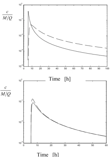
The convolution can be performed for any arbitrary number of parts of any arbitrary lengths, which means that the above conclusions can even be generalised to a network scale. Consequently, if we were able to take samples from the bedrock to the extent that we are sure what properties migrating radionuclides will encounter, the auto-correlation of a rock property would not be important for the solution. However, the variance of the properties is important for the solution. Fig. 1 shows how the solution varies between a case in which when we consider the variance in the properties (solution is obtained as E[S]) and when the properties are represented using expected values (solution is obtained as S(E[KD];E[ε];E[εt];E[u];E[h])). The difference is generally not so great even if all

properties vary and, for moderate variances, we can use the expected values of the properties as approximations.

0 10 20 30 40 50 60 70 80 90 100 10-4 10-3 10-2 10-1 100 0 10 20 30 40 50 60 10-3 10-2 10-1 100

Fig. 1 Solution according to (18) to transport in a fracture in which the properties are different in two half-parts (solid curves) and the solution according to (16) with expected value of the individual parameters (dashed curve). In the left-hand diagram the effective diffusivity Dp varies a factor 10 between the two half-parts. In the right-hand diagram the

fracture aperture h varies a factor 10 between the two half-parts. The largest values of Dp

and h were 1x10-9 m2/s and 2x10-3 m. Further, u = 0.198 m/h, KD = 540, εt = 0.004 and ε

= 0.006.

2.4 Evaluation of Covariance Structures of Transport Properties of Crystalline Rock and Implications to Solution Procedure

An important problem for interpretation of modelling results is due to the fact that measuring programmes generally provide discrete information on a large set of physical and geochemical parameters. The discrete data sampling leads to a need to “interpolate” between known data and this introduces significant uncertainties in a transport analysis

Time [h] Time [h] Q M c Q M c

similarly as there is an uncertainty in the water flow analysis. The uncertainty analysis is based on theory for stochastic processes and further discussed in section 2.5. One of the key statistical measures that appear in the stochastic analysis is the auto-covariance function of the different rock properties. This section focuses on how auto-covariance of the different properties can be expressed in terms of the auto-covariance of the auxiliary variable β and how this can be related to data.

Since the matrix properties are nested with each other and with the Laplace variable p in (13), the auto-covariance of the β can be rather complicated when equated in terms of the auto-covariances of the individual rock properties. Here we will explore the

approximation using a "Simple Approach" (Wörman et. al., 2003), which is to assume that the stochastic components of the β are represented as if the sorption kinetics is rapid (kr

→∞ ) and the permissible depth of matrix diffusion is infinite (Z →∞). The approximation is reasonable for short transport distances, because then perturbations introduced inside the exponential function of (12) contributes only insignificantly to the perturbations in the β. Hence, the stochastic components of the β can be isolated in three factors ηu(x), ηh(x) and

ηM(x) containing ˜ ε ,˜ ε t, ˜ D p, ˜ h , ˜ u and K ˜ D, where ηu≡u/˜ u , ηh≡h/˜ h , ηM≡ ˜ M / M , M =

(D_pεtε(1+ KD))

0.5 _{[m s}-0.5_{] and variables without 'tilde' are expected values (e.g. u =}

E[ ˜ u ]). We may rewrite (12) as ˜

β = c1ηu+ c2ηuηhηM (19)

in which c1 and c2 are defined in Table 1.

According to the derivation in Appendix 2, the auto-covariance of β defined

according to (19) will contain seven auto-covariance terms (A2-4). The auto-covariance of β also includes a large number of cross-covariances that could readily (from an analytical point of view) be included in the analysis, especially, if they are written in a form

appropriate for the convolution integral (27). How many terms should be included in the series is a matter of judging the importance of the terms and practical possibilities of measuring the individual factors. The solution of the convolution integral (27) is not obstructed significantly, however, by the number of terms considered. Nor is the moment

calculation or the Laplace inversion, since the Laplace variable 'p' has been separated from the η´s in (19).

In this study, we neglect the cross-covariances due to the lack of relevant data and the extensive administrative task of accounting for the cross-covariances described in Appendix 2 and especially their contributions to the ai-factors in Table 1. Further, the

cross-covariances are always smaller than the auto-covariance of an individual factor and, therefore, of lesser importance.

Geostatistics of fracture apertures and rock properties such as porosity, effective diffusivity and sorption capacity were investigated by Hakami and Barton (1990) and Xu & Wörman (1998) on rock samples taken from Äspö Hard Rock Laboratory in Sweden. Both investigations show that the auto-covariance functions of aperture and effective matrix parameter can be described by an exponential function. Thus, the covariance function β can be expressed as a series of exponential functions with different ai and

correlation length li corresponding to the different rock properties:

Cov ˜

[ ]

_β

( )

s = a_ie−s li

i=1 7

∑

(20)

where ai and li are defined in Table 1.

Table 1 Definition of typical coefficients in Eqs. (19) and (20).The _α is defined based on expected values of the included parameters.

c₁ =p u c2 = − 2εtDp hu α 1 − 2 1+ exp −2Zα

(

)

      i ai bi l_i 1 (c1+E

[ ]

ηh E

[ ]

ηM c2)2 b1 Var

[ ]

ηu lu 2 (c2)2 b2 E2

[ ]

η_u E2

[ ]

η_M Var

[ ]

η_h l_h 3 (c2)2 b3 E2

[ ]

η_u E2

[ ]

η_h Var

[ ]

η_M l_M 4 (c2)2 b4 E2

[ ]

η_u Var

[ ]

η_h Var

[ ]

η_M M h l l 1 1 1 + 5 (c2)2 b5 E2

[ ]

η_h Var

[ ]

η_u Var

[ ]

η_M M u l l 1 1 1 + 6 (c2)2 b6 E2

[ ]

η_M Var

[ ]

η_u Var

[ ]

η_h h u l l 1 1 1 +

7 (c2)2 b7 Var

[ ]

ηu Var

[ ]

ηh Var

[ ]

ηM

M h u l l l 1 1 1 1 + +

2.5 Methodology of solving one-dimensional stochastic solute transport problem This section focuses on using the spectral method to obtain solutions of the stochastic transport problem both in terms of a closed-form solution in Laplace domain (following the method outlined in section 2.2) and temporal moments of the travel time PDF. The

temporal moments of the travel time PDF are generally considered to be typical quantities of solute transport and are often obtained by the way of Laplace transforms (e.g. Espinoza and Valocchi, 1997). The temporal moments can be interpreted as "effective" transport properties such as mean residence time and variance of the residence times and are suitable for incorporation in large-scale transport models or directly in the safety assessments of the nuclear waste repository (Cvetkovic and Selroos, 1999).

By defining _β ˜

( )

p as a stochastic variable we define the stochastic properties of (11) as the sum of their expected value (or ensemble average), denoted by E[...], and random perturbations deviating around the mean, denoted by a prime;

˜

β

( )

p,x ≡ E ˜

[

β

( )

p,x

]

+β′ p,x

( )

(21)

c p,x

( )

≡ E c p,x

[

( )

]

+ ′ c p,x

( )

(22)

The definition (21) implies that

E

[ ]

_β′ = 0 (23)

Similarly, we have E[ c ′ ] = 0. In terms of perturbations the governing equation (11) can thus be written as

∂E c

[ ]

∂x +

∂c ′

The expected value of (24) under consideration of (23) yields

∂E c

[ ]

∂x + E ˜

[ ]

β E c

[ ]

+ E

[ ]

β′ ′ c s= 0= 0 (25)

in which s is the separation distance between the locations along the x-direction of β´ and c ′ . Expression of the cross-covariance between β´ and c ′ (for s=0) is known as the "closure problem".

A perturbation equation is obtained by subtracting (25) from (24);

∂c ′

∂x + E ˜

[ ]

β c ′ +β′E c

[ ]

+β′ ′ c − E

[ ]

β′ ′ c s= 0= 0 (26)

The last two terms of (26) representing perturbations of second order can be omitted if their sum is small in comparison to other terms of the equation (e. g. Espinoza and Valocchi, 1997). Therefore, the last two terms of (26) are neglected in the subsequent analysis.

By using a spectral representation (Fouries-Stiltjes integrals) of the stochastic variable of (26) we can derive the expression of the cross-spectral density function of β´ and c ′ in Fourier-space (Appendix 1). Transformation to the real domain yields:

Cov

[

_β′ x + s

(

)

,c x′

( )

]

= −E c

[ ]

∫

_−∞∞β′ s −

(

ζ

)

e−E ˜ [ ]β ( )s−ζ Cov

[

_β′ s =

(

ζ

)

]

d_ζ (27) in which θ(s) is the Heaviside unit function, ζ is the convolution integrand and cov[β´(s)] is a short form of cov[β´(x),β´(x+s)] that is used under the assumption of stationarity of the covariance function. As before, s is the separation distance along the x-direction.

If (20) is inserted in (27), we obtain Cov

[

_β′ x

( )

,c x′

( )

]

s= 0= E

[

β′, ′ c

]

s= 0= −E c

[ ]

ai li E ˜

[ ]

_{β li}+1 i=1 7

∑

(28)

in which the amplitudes ai and the correlation lengths l_i are defined in Table 1. The

solution of (25) and (28) using the boundary condition (7) becomes

E c

[ ]

=M0

Q exp −E ˜

[ ]

β + _i=1ai

N

∑

li E ˜

[ ]

_{β li}+1         x         (29)

in which N=7 for the solution in a single fracture and N=26 for the solution in a network scale.

The uncertainty of the mean value solution can be expressed from the solution of the perturbation equation (26). By substituting (29) in (26) and using the boundary conditions

c ′(x = 0)= 0, we may derive ′ c = M0β′ Q a_i li E

[ ]

_β′li+1 i=1 N

∑

exp

(

−E ˜

[ ]

β x

)

1− exp ai

li E ˜

[ ]

_{β li}+1 i=1 N

∑

                (30)

in which β´ is defined in Appendix 2.

Unfortunately, this solution in the Laplace domain cannot be inverted in closed form according to the best of the authors´ knowledge. Therefore, the series expansion method of De Hoog et al. (1982) was applied in a numerical inversion algorithm using the

MATLAB code written by Hollenbeck (1998). The accuracy of the numerical inversion was tested by means of comparisons with a closed-form solution (Neretnieks 1980) for the case with homogeneous parameters and equilibrium sorption.

The application of (10) to (29) involves a series of tedious but also relatively simple operations, which lead to the following expressions for the central temporal moments:

µt =

x

σt 2 ₌2 3 x uRTE

[ ]

ηu E

[ ]

ηh E

[ ]

ηM 1+ Ψ1+ 3R 1+ E η

[ ]

h E

[ ]

ηM R

(

)

2 R2 Hi i=1 N1

∑

+ H_i i= N2 N₃

∑

                  (32) S_t = 4 5 x uRT 2_{E η} u

[ ]

E

[ ]

ηh E

[ ]

ηM 1+ 5Ψ1Ψ2 + 5 2 1+ E η

[ ]

h E

[ ]

ηM R

(

)

R     Hi i=1 N1

∑

3E2 _η u

[ ]

E

[ ]

ηh E

[ ]

ηM H_i b_i i=1 N1

∑

(

1+ E η

[ ]

h E

[ ]

ηM R

)

2 + 2E η

[ ]

h E

[ ]

ηM R 1

(

+ Ψ1

)

     _   + +5 2 Hi 3 H_i b_i E 2 _η u

[ ]

E

[ ]

ηh E

[ ]

ηM

(

1+ E η

[ ]

h E

[ ]

ηM R

)

R+ 2R + 2RΨ1      _        _   i= N2 N3

∑

    (33)

in which N1=1, N2=2 and N3=7 for the solution in a single fracture and N1=2, N2=3 and

N3=26 for the solution in a network scale, the typical parameters R, T, Ψ1, Ψ2 and Hi are

defined in Table 2, all of which are expected values. The effect of the uncertainty of the parameters in a heterogeneous bedrock is reflected in the H-parameters. The E[ηi]

coefficients represent the effect of the actual (known) variability in parameters that exists even if there is no uncertainty about the distribution of properties along a specific transport path. The homogeneous case is obtained for Hi = 0 ; i = 1,2…7. The ψ−parameters reflect

the kinetics of the sorption process and can be disregarded in the case of equilibrium sorption (ψ1 << 1).

From (31), the travel velocity is linearly proportional to the advection velocity according to dx/d_{µt = u/(1 + R), in which R can be interpreted as a retardation factor. The} retardation coefficient reflects the mass ratio of the solute that on the average is resident in the rock matrix and the main fracture, respectively. The variance of the travel time PDF increases linearly with the retardation coefficient and the typical residence time, T, for the solute in the rock matrix. From (31) we may also conclude that the heterogeneity of the problem parameters (fracture aperture, fracture velocity, matrix diffusivity, bedrock porosity and sorption partition coefficient) does not affect the mean residence time. However, there is a corresponding positive contribution to both the variance and the skewness of the residence time.

Table 2 Definition of typical parameters governing the propagation of a solute pulse in a fracture. R =2Zε h

(

1+ KD

)

T= ε εt Z2 D_p

(

1+ KD

)

Ψ1 = 3K_D Tk_r

(

1+ KD

)

Ψ2 = K_D 3 1

(

+ KD

)

+ 1 2Tk_r + 1 3 1

(

+ KD

)

H_i = li bi E

[ ]

ηu E

[ ]

ηh E

[ ]

ηM u T

where _li and bi are defined in Table 1 and Table

A3-1 depending on the solution if it is for single fracture or network scale.

2.6 Extending the solutions to a network scale

The convolution integral (1) can be applied to a distribution of pathways both in a two dimensional fracture and in a network or a two-dimensional fracture network. The latter problem is more general and, therefore, focused on in this section.

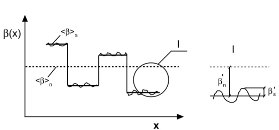
Fig. 2 presents a schematic of the variation of β along the network of fractures and illustrates the shift of the local mean values of β between fractures around the mean value of β for the whole network. In addition, within each fracture the β varies around its mean value. Hence, the perturbation of β in (21) includes two parts:

E ˜

[

_β

( )

p,x

]

+β′ ≡ E ˜

[

β

( )

p,x

]

+βn′

( )

p,x +βs′

( )

p,x (34)

in which _βn' _{denotes a random perturbation of the mean value of individual fractures}

around the mean aperture of the ensemble of fractures and _βs' _{denotes the random}

perturbation around the mean value of the individual fracture (Fig. 2).

To solve (11) with β expressed according to (34) we can follow exactly the same procedures as described before. However, the expression of covariance of β'(s) will be 26 terms instead of 7 terms according to the derivation of Appendix 3. The solutions are given on the same form as (31), (32) and (33), but the expected values of various parameters are defined as mean values of the network and the H-parameters are defined in Table 2 and Table A3-1 in Appendix 3.

β(x)

x

β'_n s β ' <β> <β>s n

I

_I

Fig. 2 Definition sketch of perturbation of _β along the pathway in a fracture network, in which, <_β>s denotes the mean value of the single fracture, <β>n denotes the mean

value of the ensemble of fractures in the network, _βn' _{and β}

s

' _{denote the perturbation}

2.7 One-Dimensional Continuum Model

Section 3.4 contains a comparison in result between the multi-dimensional description of the water flow and solute transport, explored in this study, and the classical one-dimensional continuum description of solute transport by groundwater as given by the Advection-Dispersion equation. This comparison is introduced to demonstrate the importance of the multi-dimensional approach for certain field conditions. For a continuous Darcy velocity field, the one-dimensional solute transport mechanism can be described by [SKI, 1996],

Mobile phase in pore water

∂c ∂t

( )

θRc + q ∂ c ∂x− ∂∂x θD ∂ c ∂x     _  = aθmDm ∂ ∂zcm z= 0−λθRc (35)

Immobile phase in the rock matrix ∂

∂t

(

Rmcm

)

= Dm

∂2_c m

∂z2 −λRmcm (36)

were the retardation factors due to surface sorption and sorption into the rock matrix is defined R=1+ kd,fρ

(

1−θm

)

aδ θ (37) R_m =1+kdρ

(

1−θm

)

θm (38) and

c = concentration of radionuclide i in the pore water [kg/m3] cm = concentration of radionuclide i in the matrix water [kg/m3]

q = groundwater flow (Darcy velocity) [m3/ m2/s] D = dispersion coefficient for porous media [m2/s]

a = specific flow wetted area of fractures (per volume rock mass) [m-1] w = distance into matrix orthogonal to fracture surface [m]

Dm = matrix diffusivity [m2/s]

kd,f = sorption coefficient for radionuclide i for the fracture surfaces [m3/kg]

kd = sorption coefficient for radionuclide i inside rock matrix [m3/kg]

δ = ‘depth’ of surface sorption [m] θ = rock mass (‘flowing’) porosity [-] θm = matrix porosity [-]

λi = decay constant for radionuclide i [s-1]

ρm = bulk density of rock matrix [kg/ m3]

With the same initial and boundary conditions as (5) to (8) a solution to equations (35) and (37) can easily be found in the Laplace domain following a series of simple steps:

c =M Qexp qx 2_θD 1− 1+ 4D_θ2 q2 R p

(

+λ

)

− a_θmD_m θ α 1− 2 1+ exp −2

(

αz

)

                              (39)

where the auxiliary variable is defined as

α = Rm

(

p+λ

)

D_m

The inversion of equation (39) to the real time domain cannot be obtained analytically to the best of the author’s knowledge. Instead, a solution is obtained with a numerical inversion algorithm based on the series expansion method of De Hoog et al., (1982).

3. Illustrative application based on a discrete-feature model

For the purpose of illustrating the travel-time approach and comparing with the 1-D continuum model for transport, in this chapter illustrative cases are developed based on a 3-D discrete-feature model that was developed and tested in SKI’s SITE-94 performance-assessment study (SKI, 1996).

Monte Carlo simulations of the flow field and particle tracking is used to obtain the expected value of the residence time PDF, g(τ), of inert water parcels travelling through fracture networks from damaged canisters and to discharge locations. The transport paths for a non-sorbing, conservative tracer, not affected by matrix diffusion, are calculated by the discrete-parcel random-walk method. Based on the residence time PDF obtained from the particle tracking procedure, the water flow is coupled with the solute transport analyses of section 2.5 using the method of section 2.1. The information obtained by this approach is also translated to hydrological parameters used in the one-dimensional continuum modelling (i.e. Darcy velocity, effective longitudinal dispersion coefficient, flow porosity and flow wetted surface).

Examples of hydrological properties derived from the simulations of transport in the fracture network are illustrated in section 3.2. A comparison of the two approaches is performed in section 3.3. This section also focuses on effect of uncertainty in

heterogeneous rock properties on radionuclide transport. A combination of effect of flow and uncertainty due to heterogeneous rock properties is discussed in section 3.4.

3.1 Discrete-feature model for water flow analysis

The 3-D discrete-feature (DF) model used in this application consists of three major types of components [Geier, 1996]: 1) large-scale transmissive structures, including fracture zones and single fractures more than 50 m in extent, 2) smaller-scale fractures in the vicinity of the repository, and 3) man-made hydrologic features in the repository, including the disturbed-rock zone (DRZ) around the repository tunnels and shafts (see Fig. 3).

The large-scale structures along with the man-made features are treated as

realisations of the model), and with hydraulic properties that may be treated as either deterministic or stochastic depending on the calculation case.

The small-scale fractures are treated as a stochastic population of disc-shaped fractures (approximated by polygons in the model), defined in terms of a stochastic process for the location of fracture centers, and statistical distributions for other fracture properties (e.g. radius, orientation, and transmissivity). Realizations of the small-scale fracture population are generated by unconditional Monte Carlo simulation.

For each calculation case, multiple realizations of the integrated model are formed by combining realizations of the smaller-scale fracture population with the large-scale

features. For each realization, the DF model is assembled and discretized to produce a finite-element mesh, composed of triangular elements, which represents all connections among the discrete features. Boundary conditions (fixed-head, fixed flux, or fixed net flow) are imposed at the intersections between the discrete features and the model boundaries.

The steady-state hydraulic head field resulting from the prescribed boundary conditions is calculated for each realization by the Galerkin finite-element method. The velocity u within each element is calculated from the hydraulic head distribution as:

T h H T∇ − = u (40)

where H is the hydraulic head, T is the transmissivity of the element, and hT is an effective

Fig. 3 Components of the SITE-94 discrete-fracture model (Geier, 1996).

3.2 Simulations of hydrological properties of a discrete-fracture network

The demonstration case presented in this section is based on a 3-D discrete-feature model of a 5 km by 5 km area, 1 km deep and geological information obtained from the Äspö Hard Rock Laboratory site in south-eastern Sweden (Geier, 1996). Large-scale,

deterministic features in the model represent regional and local-scale fracture zones that were identified by interpretation of topographical and aerial geophysical data, combined with ground-based geophysics and borehole data. A few of these features which are intersected by boreholes have been characterized by hydrologic tests, including one suite of radially convergent tracer tests, which help to constrain the flow and transport properties of these features.

The smaller-scale fracture population in the detailed portion of the model is described based on statistical interpretation of fracture geometry data from outcrops and boreholes, and detailed hydrologic testing in boreholes. Statistical summaries of the fracture populations in the two main lithologic types in this location are given in Table 3. In both cases, analysis of fracture data indicated that nonuniform clustering of fractures cannot be described as a uniformly random Poisson process for fracture center location, but is more closely

Table 3. Statistical summary of models for fracturing in the repository block. Orientation

distributions are defined by bootstrap resampling of Terzaghi-corrected datasets, for all fracture sets. Fracture location Fracture transmissivity Lognormal Fracture radius Power-law

Rock Type Fracture

Set DLL (-) P32c (m2_/m3_{) (log}λlog T 10 m2/s) ρlog T (log10 m2/s) br (m) All 0.799 -1 0.314 3.00 2 0.163 3.01 3 0.138 2.74 Äspö granodiorite 4 2.23 0.184 -8.5 1.0 2.55 All 0.427 -1 0.159 3.00 2 0.086 3.01 3 0.082 2.74 Småland granite 4 2.14 0.100 -8.0 1.25 2.55

approximated by a fractal (3-D Levy flight) process, which is characterized in terms of a fractal dimension DLL for the point field of fracture centers. The intensity of fracturing in

the models is described in terms of the total interfacial area of conductive fractures per unit volume of rock, P32c [m2/m3].

Four fracture sets were identified based on orientation: (1) NW to NNW strike, steeply dipping, (2) NE strike, steeply dipping, (3) subhorizontal, and (4) N-S strike, steeply dipping. The orientations of the simulated population of fractures were generated by bootstrap resampling of fracture pole data from outcrop mapping, after a correction for directional sampling bias.

Fracture transmissivity for all sets was modeled by a lognormal distribution,

estimated by forward modeling of the observed distribution of 3 m section transmissivities based on the inferred model for fracture clustering. Thus transmissivity was assumed to be independent of orientation and fracture size.

Fracture size (i.e. the radius of the discs) for all four fracture sets, for both rock types, was found to follow a power-law distribution. Thus both the fracture size distribution and fracture location process were inferred to have self-similar (fractal) properties, although it was not positively demonstrated that the fracture population as a whole was a fractal.

This statistical model was partly verified by simulation of transient hydraulic tests on 3 m sections, which showed that the model reproduced the observed distributions of both section transmissivity and flow dimension. However, it seems likely that other

combinations of statistical parameters could also reproduce these attributes ofthe fracture network. Thus this model should be regarded as one in a locus of possible models that have the capacity reproduce, in a statistical sense, the transient behavior of the fracture network over the scale affected by these hydraulic tests (likely a few meters).

For particle-tracking runs, the effective transport aperture bT in the stochastic fracture

population was also required. A correlation to hydraulic aperture bh was assumed, based on

a regression analysis of single-fracture flow and transport experiments in the literature: bT = 10-1.35 bh0.44

where both apertures are in units of meters, and where bh is by definition calculated from

the fracture transmissivity T according to the cubic law: bh = (12λT / θg)1/3

where λ and θ are the viscosity and density of water, respectively.

The model also includes conductive features associated with the backfilled shafts and tunnels of a hypothetical repository located under the island of Äspö (Figure 4). The entire repository layout was included in the model for the purpose of modelling fluid flow within and around the repository, but only 40 of the spent-fuel canister locations in this repository were modeled as potential sources of radionuclides for transport modelling as described below.

Fig. 4 Layout of shafts, access tunnels, and deposition tunnels for spent-fuel canisters, in

the hypothetical repository considered in the discrete-feature modelling example.

Fig. 5 Representation of the advective-dispersive motion in a single step of the DPRW

algorithm, within a single, linear finite element.

u x₃ x1 x₂ r u∆t ∆x=u∆t+r

For each realization of the flow field and for each of forty spent-fuel canister

locations (deposition holes), the discrete-parcel random-walk (DPRW) method was used to model advective-dispersive transport through water-conducting features in the discrete-feature model. Particles were tracked from the deposition hole boundary until they crossed a monitoring horizon 50 meters below the ground surface, at which point the radionuclide particles were considered to have reached the biosphere for the purposes of the SITE-94 safety-assessment exercise.

Forty canister locations act as potential sources in a hypothetical repository. Particles representing arbitrary masses of solute are released along the edges of fractures that

intersect the deposition holes. The initial positions of the particles are chosen randomly and in proportion to the flow-rate exiting in the deposition hole through each fracture, relative to the total flow through the deposition hole.

The motion of a particle within an element is modeled as a 2-D random walk (Fig. 5). Since in the discrete-feature model the aperture is modelled as a having a constant value within a given element (assumed to represent an effective average over that scale), the random walk is used to account for local hydrodynamic dispersion resulting from the combined effects of molecular diffusion, shear dispersion, and heterogeneity of physical aperture on smaller scales.

In the random walk, the displacement of the particle ∆x for a given time step ∆t is the vector sum of a deterministic, advective component u∆t and a random, dispersive component r. Here u is the local fluid velocity (assumed to be an average over the scale of the element). The time step ∆t for each increment of particle motion in the random walk is chosen based on the ratio of fluid velocity to element size.

The dispersive component r is a random vector sampled from a bivariate normal distribution of displacements from the origin, with principal components aligned with the longitudinal (parallel to flow) and transverse directions, and component variances equal to 2DL∆t and 2DT∆t, respectively. The dispersion coefficients DL and DT are assumed to be

functions of the magnitude of the local velocity (de Marsily, 1986):

) , max( _{L m}

L u D

) , max( _{T m}

T u D

D = _α (42)

where αL and αT [m] are the longitudinal and transverse dispersivities, respectively, within

a given fracture, and Dm is the coefficient of molecular diffusion (0.02x10-9 m2/s for

common ions in water).

The ratio αT/αL is assumed to be constant through out the network. For the

transport simulations described below, αT/αL is set equal to 0.1. This value is within the

typical range of 0.01 to 0.2 in porous media (Marsily, 1986). If αL is known DL and DT can

be calculated according to (41) and (42). Determination of αL will be discussed in Chapter

4.

3.3 Extraction of parameters for one-dimensional solute transport

Parameters for one-dimensional solute transport models can be extracted straightforwardly from a hydrologic model, by recording the particle position x and the local parameter values of interest (T, h, u) as functions of x for discrete time intervals and then using the statistics of these along with the inert-particle travel time distributions as input to the one-dimensional model.

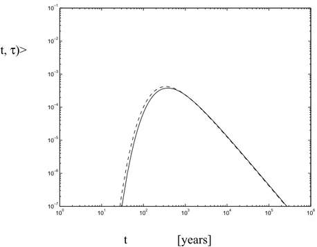
As a simplest case, parameters can be deduced from hydrologic scoping calculations based on simplifying assumptions. Fig. 6 shows the result of g(τ) taken from SITE-94 far field scoping calculation case 1a3 (SKI, 1996, p497). This scoping calculation is based on a highly simplified model of hydrology, which considers just the possible range of head differences at the site, and effectively 1-D flow and transport paths with homogeneous properties.

More complex travel-time distributions can result from 3-D flow systems in a fracture network. Branching and multiply-connected pathways within a network (which might possibly be coupled by lateral diffusion within fractures and mixing at fracture intersections, even though the paths represent different streamlines) can give rise to more complicated travel-time distributions. Figure 7 shows a case with multi-peak behaviour giving distinctly different travel times for different fractions of the particles released from a single source canister.

0 0.5 1 1.5 2 2.5 3 0 0.005 0.01 0.015 0.02 0.025 0.03 0.035 0.04

Fig. 6 Residence time PDF of inert water parcels from a single canister through the

fracture network to the biosphere, in which x=100 m, u=140 m/y and E=140 m2/y. The curve is fitted to results obtained in SITE-94 far field scoping calculation cases 1a3 (SKI, 1996, p. 497) 0 2 4 6 8 10 12 14 16 18 20 0 0.1 0.2 0.3 0.4 0.5 0.6 0.7 0.8 0.9 1

Fig. 7 Example of cumulative residence time PDF showing a multi-peak behaviour. In the

figure, the dashed line denotes the simulated g(_τ) according to case SKI0/NF0/BC0 Run 6 Source 13 (Geier, 1996) and the solid line denotes the fitted 1-D model, where the values are x=500 m, u=63 m/y and E=120 m2/y.

g(τ) Time [years] Cumulative probabilit y densit y Time [years]