2008:09 The Generalised Ecosystem Modelling Approach in radiological assessment

The Generalised Ecosystem Modelling

Approach in Radiological Assessment

Richard Kłos

SSI Rapport

2008:09

Rapport från Statens strålskyddsinstitut tillgänglig i sin helhet via www.ssi.se

Ultraviolet, solar and optical radiation

Ultraviolet radiation from the sun and solariums can result in both long-term and short-term effects. Other types of optical radiation, primarily from lasers, can also be hazardous. SSI provides guidance and information.

Solariums

The risk of tanning in a solarium are probably the same as tanning in natural sunlight. Therefore SSI’s regulations also provide advice for people tanning in solariums.

Radon

The largest contribution to the total radiation dose to the Swedish population comes from indoor air. SSI works with risk assessments, measurement techniques and advises other authorities.

Health care

The second largest contribution to the total radiation dose to the Swedish population comes from health care. SSI is working to reduce the radiation dose to employees and patients through its regulations and its inspection activities.

Radiation in industry and research

According to the Radiation Protection Act, a licence is required to conduct activities involving ionising radiation. SSI promulgates regulations and checks compliance with these regulations, conducts inspections and investigations and can stop hazardous activities. Nuclear power

SSI requires that nuclear power plants should have adequate radiation protection for the generalpublic, employees and the environment. SSI also checks compliance with these requirements on a continuous basis.

Waste

SSI works to ensure that all radioactive waste is managed in a manner that is safe from the standpoint of radiation protection.

Mobile telephony

Mobile telephones and base stations emit electromagnetic fields. SSI is monitoring developments and research in mobile telephony and associated health risks.

Transport

SSI is involved in work in Sweden and abroad to ensure the safe transportation of radioactive substances used in the health care sector, industrial radiation sources and spent nuclear fuel.

Environment

“A safe radiation environment” is one of the 15 environmental quality objectives that the Swedish parliament has decided must be met in order to achieve an ecologically sustainable development in society. SSI is responsible for ensuring that this objective is reached.

Biofuel

Biofuel from trees, which contains, for example from the Chernobyl accident, is an issue where SSI is currently conducting research and formulating regulations.

Cosmic radiation

Airline flight crews can be exposed to high levels of cosmic radiation. SSI participates in joint international projects to identify the occupational exposure within this job category.

Electromagnetic fields

SSI is working on the risks associated with electromagnetic fields and adopts countermea-sures when risks are identified.

Emergency preparedness

SSI maintains a round-the-clock emergency response organisation to protect people and the environment from the consequences of nuclear accidents and other radiation-related accidents.

SSI Education

SSI rapport: 2008:09 mars 2008

ISSn 0282-4434

The conclusions and viewpoints presented in the report are those of the authors and do not necessarily coincide with those of the SSI.

Författarna svarar själva för innehållet i rapporten.

edItorS / redaktörer : Richard Kłos

tItle / tItel: The Generalised Ecosystem Modelling Approach in radiological

assessment/ Generaliserad ekosystemsmodellering för radiologisk konsekven-sanalys

department / avdelnIng: of Nuclear Facilities and Waste Management /

Foreword

This report presents biosphere modelling in support of the review of the Swedish Nuclear Fuel and Waste Management Co’s (SKB) safety report SR-Can carried out by SSI’s modelling team, CLIMB. The CLIMB review report (SSI Report 2008:08) is, in turn, a supporting document for the joint review of SR-Can by SSI and the Swedish Nuclear Power Inspectorate (SKI). The authorities review report is published in a joint SSI/SKI report (SSI Report 2008:04 E; SKI Report 2008:23).

SKB plans to submit a license application for the construction of a repository for spent nuclear fuel in Sweden 2010. In support of this application SKB will present a safety report, SR-Site, on the repository’s long-term safety and radiological consequences. As a preparation for SR-Site, SKB published the preliminary safety assessment SR-Can in November 2006, documenting a first evaluation of long-term safety for two candidate sites Forsmark and Laxemar.

An important objective of the authorities’ review of SR-Can is to provide regulatory guidance to SKB on the complete safety reporting for the license application. The

authorities have engaged external experts for independent modelling, analysis and review, with the aim to provide a range of expert opinions related to the sufficiency and

appropriateness of various aspects of SR-Can.

This report presents model development and modelling carried out by SSI’s consultant, Richard Kłos. A generic modelling approach has been developed and used as a means of evaluating the radiological impact of radionuclide release to the surface environment in SKB’s SR-Can assessment. The conclusions and judgements in this report are those of the author and may not necessarily coincide with those of SKI and SSI. The authorities own review will be published separately (SKI Report 2008:23, SSI Report 2008:04 E).

Förord

Den här rapporten redovisar biosfärsmodellering som utförts till stöd för SSI:s modelleringsgrupp CLIMB i dess granskning av Svensk Kärnbränslehantering AB:s (SKB) säkerhetsredovisning SR-Can. CLIMB:s granskning (SSI Rapport 2008:08) utgör i sin tur ett underlag för SSI’s och Statens kärnkraftinspektions (SKI) gemensamma granskning av SR-Can (SSI Rapport 2008:04; SKI Rapport 2008:19).

Svensk kärnbränslehantering AB (SKB) planerar att lämna in en ansökan om uppförande av ett slutförvar för använt kärnbränsle i Sverige under 2010. Som underlag till ansökan kommer SKB presentera en säkerhetsrapport, SR-Site, som redovisar slutförvarets långsiktiga säkerhet och radiologiska konsekvenser. Som en förberedelse inför SR-Site publicerade SKB den preliminära säkerhetsanalysen SR-Can i november 2006, vilken redovisar en första bedömning av den långsiktiga säkerheten vid SKB:s två

kandidatplatser Laxemar och Forsmark. Myndigheternas granskning syftar till att ge SKB vägledning inför den planerade tillståndsansökan. Myndigheterna har i sin granskning tagit hjälp av externa experter för oberoende modellering, analys och granskning. Modelleringen som redovisas i denna rapport har genomförts av SSI’s konsult Richard Kłos. En flexibel compartment-modell har utvecklats och använts som ett verktyg för att utvärdera de radiologiska konsekvenserna från utsläpp av radionuklider till ytmiljön i SKB:s säkerhetsanalys SR-Can. Slutsatserna och bedömningarna i denna rapport är författarens egna och överensstämmer inte nödvändigtvis med SSI:s ställningstaganden.

Sammanfattning

SSI behöver en oberoende modelleringskompetens för att kunna utvärdera de

doskonsekvensanalyser som görs av SKB. Fokus ligger på utvärdering av den långsiktiga radiologiska säkerheten för slutförvar för både använt kärnbränsle och lågaktivt

radioaktivt kärnavfall.

SSI startade modelleringsgruppen CLIMB (Catchment LInked Models of radiological effects in the Biosphere) år 2004 för att utveckla nya modeller som kan användas som oberoende modelleringsverktyg i säkerhetsanalys. Ett av resultaten är utvecklingen av GEMA (generalised ecosystem modelling approach) modellen.

GEMA är boxmodeller med ett modulsystem för att beskriva radionukliders omsättning i ytmiljön. Det kan konfigureras, genom vatten- och materialflöden, för att beskriva en rad av ekosystem i det svenska landskapet. Modellen är generell, men finjustering kan göras med hjälp av lokala detaljer om ythydrologi.

The modular nature of the modelling approach means that GEMA modules can be linked to represent large scale surface drainage features over an extended domain in the

landscape. System change can also be managed in GEMA, allowing a flexible and comprehensive model of the evolving landscape to be constructed. Environmental concentrations of radionuclides can be calculated and the GEMA dose pathway model provides a means of evaluating the radiological impact of radionuclide release to the surface environment.

Modulegenskaperna innebär att GEMA-moduler kan kopplas ihop och beskriva storskaliga avrinningsområden i landskapet. GEMA tillåter även beskrivning av ett landskap som utvecklas i tiden. Miljökoncentrationer av radioaktiva ämnen kan beräknas och dosmodellen i GEMA gör det möjligt att utvärdera de radiologiska konsekvenserna av utsläpp till ytmiljön.

Det här dokumentet redovisar principerna bakom GEMA-modellen och dess

funktionalitet och illustreras med beräkningsexempel som genomförts till stöd för SSI:s granskning av SR-Can.

Summary

An independent modelling capability is required by SSI in order to evaluate dose assessments carried out in Sweden by, amongst others, SKB. The main focus is the evaluation of the long-term radiological safety of radioactive waste repositories for both spent fuel and low-level radioactive waste.

To meet the requirement for an independent modelling tool for use in biosphere dose as-sessments, SSI through its modelling team CLIMB commissioned the development of a new model in 2004, a project to produce an integrated model of radionuclides in the landscape. The generalised ecosystem modelling approach (GEMA) is the result.

GEMA is a modular system of compartments representing the surface environment. It can be configured, through water and solid material fluxes, to represent local details in the range of ecosystem types found in the past, present and future Swedish landscapes. The approach is generic but fine tuning can be carried out using local details of the surface drainage system.

The modular nature of the modelling approach means that GEMA modules can be linked to represent large scale surface drainage features over an extended domain in the

landscape. System change can also be managed in GEMA, allowing a flexible and comprehensive model of the evolving landscape to be constructed. Environmental concentrations of radionuclides can be calculated and the GEMA dose pathway model provides a means of evaluating the radiological impact of radionuclide release to the surface environment.

This document sets out the philosophy and details of GEMA and illustrates the

functioning of the model with a range of examples featuring the recent CLIMB review of SKB’s SR-Can assessment.

Contents

1.2 Outline of the report... 1

2 The GEMA module ... 3

2.1 Ecosystem types – a generic model ... 3

2.2 Transfer processes and environmental concentrations... 4

2.3 Exposure pathways ... 6

2.3.1 Basis... 6

2.3.2 Ingestion dose ... 6

2.3.3 Inhalation doses ... 7

2.3.4 External irradiation ... 7

2.4 Landscape modelling and system change ... 9

2.5 GEMA implementation... 10

3 GEMA datasets... 11

3.1 Background... 11

3.2 An evolving system: Basin Borholmsfjärden, Laxemar ... 12

3.2.1 Landscape features... 12

3.2.2 Landscape evolution at Laxemar ... 15

3.2.3 Parameterisation of water and solid material balance: transfer coefficients... 18

3.2.4 Time varying parameters ... 26

3.2.5 Borholmsfjärden extreme: small bay north of Borholmsfjärden ... 27

3.3 An extended landscape model: Lake Bolundsfjärden, Forsmark ... 31

3.3.1 GEMA flowpath elements in the Bolundsfjärden catchment ... 31

3.3.2 Data description ... 31

3.4 Nuclide specific data... 34

4 Illustrative results... 39

4.1 Evolving bays at Laxemar – modelling transitions... 39

4.2 Contaminant fate in the Bolundsfjärden drainage system ... 44

5 Summary and conclusions ... 46

References... 47

Appendix A – Generic GEMA FEP matrix ... 49

Appendix B – Solution method using direct matrix inversion... 50

Appendix C – GEMA implementation: control and datafiles... 53

Appendix D – Glossary of GEMA parameters ... 64

1 INTRODUCTION

1.1 Background

As the regulatory authority for radiological protection in Sweden SSI has instigated

Pro-jekt CLIMB – Catchment LInked Models of radiological effects in the Biosphere – as a

means of carrying out numerical assessments of the potential impact of radionuclide re-leases to the surface environment following disposal of spent fuel and other radioactive wastes in deep geologic repositories. The biosphere assessment model developed in CLIMB is GEMA – the generic ecosystems modelling approach.

GEMA provides SSI with the capability to carry out independent numerical evaluations of releases of radionuclides to biosphere systems typical of those associated with SKB’s candidate sites for a disposal facility for spent radioactive fuel. The models developed in CLIMB have been employed in a review (Xu et al., 2008) of the SR-Can assessment (SKB, 2006a).

An essential feature of GEMA is that radionuclide transport and accumulation in the bio-sphere is modelled over spatially extended regions. A modular representation of ecosys-tems within the overall surface drainage system is constructed from the GEMA modules that represent elements of the flowpath network. The modular approach also allows con-ditions in the system to change in time so that models of the evolving landscape system can be constructed.

This document provides a description of the modelling philosophy, the detail of the indi-vidual ecosystem sub-models and the application of the model.

1.2 Outline of the report

A review of SKB’s documentation of models for dose assessment prior to SR-Can, par-ticularly SKB (2004), the interim SR-Can documentation, suggested a basic modular structure for GEMA. This structure is discussed in Section 2.1 below. The representation of transfer processes in the physical transfer model is reviewed in Section 2.2 and the exposure pathways models are set out in Section 2.3. Section 2.4 describes how a land-scape model is configured using the GEMA module. It also outlines how system change can be represented.

As with many biosphere assessment models, GEMA is somewhat data intensive and this is compounded by the need to represent the extended landscape in both time and space. GEMA is intended specifically for interpretation of radiological assessments of candidate sites for geological disposal facilities proposed by SKB in Sweden. Interpretation of site data in GEMA is a key issue. Section 3 illustrates how elements of the SKB’s extensive site descriptive database are used to populate GEMA’s datasets. The GEMA models dis-cussed here are based on an independent interpretation of site descriptive data for Fors-mark and Laxemar (Lindborg, 2005; 2006). Section 3 also shows how the GEMA data-sets are constructed after identifying time invariant and time varying parameters. A full reference dataset for the exposure pathway submodel is also given for reference. To illustrate the application of GEMA, results are discussed in Section 4 featuring two objects in the Laxemar landscape and a non-evolving model of contaminant transport

through a simplified model of the present day Forsmark landscape. Section 5 has some concluding remarks.

2 THE GEMA MODULE

2.1 Ecosystem types – a generic model

At the time of the SR-Can interim assessment in 2004 (SKB, 2004) SKB had clearly identified the different types of ecosystem necessary to model the evolution of the bio-sphere at the Forsmark and Laxemar sites. For example, the 2500 AD Forsmark site was judged to comprise:

Marine areas (2 locations) Mire (6)

Lake (3) Forest (1)

Running water (1).

While this is neither exhaustive nor wholly representative of the site potentially affected by release of radionuclides at 2500 AD, the types of ecosystem are typical according to (SKB, 2006a) and the ecosystem models used are in SR-Can are similar to those de-scribed in earlier assessments (Avila, 2006). To this may be added areas of agricultural land. To offer the greatest degree of flexibility the decision was made that the CLIMB biosphere model would use a generic structure of eight compartments to allow combina-tions of terrestrial and aquatic ecosystems. This structure is shown in Figure 2.1. The terrestrial sub-model comprises upper (rooting zone) soil with a deeper soil layer overly-ing less weathered Quaternary deposits (QD). A litter layer can be modelled above the soil layers. In the aquatic sub-model sediment is represented as two layers to allow the upper sediment layer to have different characteristics from the deeper material. Further-more, to allow for modelling of deep bays and lakes there can be two layers of the water column. LWat- Lower water column TSed- Upper sediment DSed- Deep sediment UWat- Upper water column inflow outflow inflow inflow inflow outflow outflow outflow TSoil- Top soil DSoil- Deep soil Q- Quaternary deposits

Upper GBI (radionuclide source)

Litt- Litter layer

Atmosphere (water and solid material source) inflow inflow inflow inflow outflow outflow outflow outflow LWat- Lower water column TSed- Upper sediment DSed- Deep sediment UWat- Upper water column inflow outflow inflow inflow inflow outflow outflow outflow TSoil- Top soil DSoil- Deep soil Q- Quaternary deposits

Upper GBI (radionuclide source)

Litt- Litter layer

Atmosphere (water and solid material source) inflow inflow inflow inflow outflow outflow outflow outflow

Figure 2.1. The GEMA module. Elements of the flow path are represented by the eight compartments. Material flows from upstream to downstream can be included. Flows to and from the atmosphere and geosphere-biosphere interface are an inte-gral part of the mass balance scheme. The short names of the compartments illus-trated are used as suffixes when writing the GEMA equations: Q = Quaternary de-posits, LWat = lower water, etc.

The inclusion of compartments for both terrestrial and aquatic structural elements within the same modular framework allows a number of practical modelling features: all model elements have representative hydrology which allows in- as well as outflows. Mass bal-ance (for water fluxes, solid material fluxes and, automatically thereby, radionuclides) is the basis for the model representation in each module. Integration into a landscape model in which the different elements of the drainage system flowpath exchange material is therefore straightforward (see Section 2.4).

Different ecosystems representations may not require that all compartments are involved at all times. For example the litter layer is only required for modelling forest (including natural scrubland). Many mainly aquatic modules only need the lower water column (e.g., rivers, shallow lakes and bays). Compartments can be switched in and out as required during the evolution of the system.

Over short timescales evolution can be modelled by the gradual change in properties of the individual compartments. Over longer periods accounting for changes in geometry and structure can require some compartments to be turned on or off. Accounting for the accumulated contamination then requires that some inventories be transferred to other compartments within the same module. Over the longest timescales the overall nature of the ecosystem at any particular spatial location might change such that the characteristics differ completely those at the earlier time. Mass conservation requires that the inventory at the earlier time be transferred appropriately to the compartments at the later time. Both gradual (successionary) changes can be modelled – e.g., sedimentation within lakes and bay – as well as sudden changes such as the transformation of wetland areas to farm-land by human action.

The generic GEMA FEP matrix is shown in Appendix A.

2.2 Transfer processes and environmental concentrations

GEMA uses a traditional compartment modelling approach to represent radionuclides transport and accumulation in the environment. The dynamics of the radionuclide inven-tories (expressed as Bq) in the eight shown in Figure 2.1 are given by

(

)

_{( )}

where N is the vector of compartment contents (Bq) of radionuclide N and M is the con-tent of parent nuclide M. The decay constant for N is λ_N y-1 _{and external sources (inputs)}

are . Intercompartment transfers are given by the matrix y-1_{. The solution to this}

equation is implemented at SSI using Matlab®. Details are given in Appendix B.

( )

S Λ

The compartment model approach uses transfer coefficients to model the fractional trans-fer between compartments in the module. The transtrans-fer matrix Λ has elements,

λ

∑

For transfers driven by water ( m3 _y-1_{) and solid material fluxes ( kg y}-1_{) this}

becomes

ij

F Mij

Quaternary deposit, soils, sediments

(

)

The compartment volume is m3_{, with porosity}

i

V ε_i and volumetric moisture content θ_i. Density of the parent material is ρ_i kg m-3 _{and the solute – solid distribution coefficient}

is (Bq kg-1_{)(Bq m}-3₎-1_{. Equation (2.3a) allows for local variations in bulk density to be}

explicitly addressed, based on the structural properties of the compartment.

i k

Modelling in GEMA modules thus depends on the identification the environmental driv-ers – the water and solid fluxes. Each GEMA module has a water flux matrix, F m3 _y-1_,

and a solid material flux matrix , M kg y-1_{, defined. These matrices express flux}

conser-vation spatially – inflow and outflow balance is evaluated – and temporally as the com-partments change in time.

Concentration in environmental media can be calculated in a variety of ways. The most straightforward is to take the compartmental inventories, obtained from the solution to Equation (1.1), to determine the volumetric concentration:

i i i V N C = Bq m-3_{. (2.4)}

Other forms are possible but these can be evaluated from this basic definition using the compartment characteristics. For example, the unfiltered porewater concentration in com-partment i representing an aquifer is given by

(

)

(

)

which takes into account not only the dissolved radionuclide but also the amount sorbed into suspended solid material present in the porewater as suspended solid load kg m-3. The concentration per wet weight or dry weight soil can be found by similar manipulation of Equation (2.4).

i α

2.3 Exposure pathways

2.3.1 Basis

Evaluation of annual individual dose requires an estimation of the degree of interaction between contaminated media and hypothetical individuals comprising the “critical group” on an annual basis1_{. Exposure is via ingestion, inhalation or external irradiation and each}

of these are related back to the concentrations given by Eq. (2.4). Ingestion includes all pathways entering through the gastrointestinal tract including foodstuffs and water as well as any direct consumption of soil particles. Inhalation doses are via radionuclides

breathed into the lungs. External irradiation accounts for contaminated environmental media exposing the body of exposed individuals.

2.3.2 Ingestion dose

Ingestion doses are calculated using the dose conversion factor for ingestion, Hing Sv Bq-1,

to evaluate the annual dose on the basis of annual intake:

Sv y-1_{, (2.6)} k k ing k H I C D =

as (kg y-1) is the annual intake of medium k with concentration (Bq kg-1 or Bq m-3_).

k

I C_k

Intake rates are largely determined by diet of different foodstuffs available from the eco-system module but foodstuff concentrations are related to the media concentrations. Both soil and water concentrations might be involved in the production of a particular food-stuff. For example, accumulation in cultivated crops might involve the top soil together with well, lake or river water if the crop is irrigated. Animals might consume locally pro-duced foodstuffs as well as water. Local conditions in the ecosystem determine which media are involved.

In general the expression for the concentration in foodstuff k is given by:

1 _{The “critical group” concept is used here to indicate a group of individuals for whom}

radiological exposures are the highest within the societal context of the modelled system. The usage is synonymous with the “most exposed group” and assumes a pattern of behaviour which maximises exposure to foodstuffs and other environmental media in a realistic manner. That all of the exposure pathways are assumed be active at these rates of exposure makes them

Bq kg-1 _{or Bq m}-3_{. (2.7)}

∑

The elements are the processing factors which convert the environmental distribution of radionuclides into concentrations in ingested material. The way they are calculated in GEMA is shown in

ki P

Table 2.1. The foodstuff types associated with the different ecosys-tems are shown in Table 2.2.

2.3.3 Inhalation doses

Inhalation comes only from suspended dust derived from the top soil or a combination of the top soil and litter layers in the forests:

∑

∑

H Sv Bq-1 is the dose per unit intake on inhalation and hours y-1 _{the occupancy of}

ecosystem e. The breathing rate is m3 _hour-1 _{and the dust concentration in air is}

e O b

I α_air kg

m-3_{. The average concentration in air is based on the dry concentration in both TSoil and}

Litt,

(

)

Like inhalation, external irradiation uses an occupancy factor:

∑

∑

which uses the wet soil concentration:

(

)

Table 2.1. GEMA processing factors for ingestion pathways.

Type Pathway Expression Comments

Surface water

i i

dw _V

N

C = Lakes or rivers, i = LWat or Uwat _{depending on the water body} concerned. Water c ons ump tio n Well water ( ) i i i i i i i i well _V N k k α C ρ ε θ + − + = 1

1 Aquifer: usually in the Quaternary

deposits, compartment Q. Root uptake ( ) i i i i crop root crop _V N K C ρ ε − = 1

1 Crops contaminated by root uptake,

grown on TSoil or Litt (fungi in forest areas). Uptake factor for wet soil Irrigation interception

(

)

Irrigation deposition intercepted by plant and incorporated in edible tissues. Concentration and amount of irrigation derived from aquifer or surface water

Plant pro duc e Soil ( ) i i LWat i i i soil _V N C ρ ε ρ ε + − = 1

1 Inadvertent consumption of dry soil

Meat ⎥ ⎦ ⎤ ⎢ ⎣ ⎡ + + =

∑

∑

C Combination of contaminated plant _{material, water (stream or well) and soil}

intake and distribution coefficient for meat Anim al prod uc e Milk ⎥ ⎦ ⎤ ⎢ ⎣ ⎡ + + =

∑

∑

C Combination of contaminated plant _{material, water (stream or well) and soil}

intake and distribution coefficient for milk

Table 2.2. Plant and animal products consumed by ecosystem type. Food types are those identified by SKB (2001; 2004) and for which Karlsson et al. (2001) give uptake and concentration factors.

Ecosystem Food type, k

Sea Fish

Lake Fish, freshwater invertebrates Stream Fish, freshwater invertebrates Forest Game, fruit, nuts, berries, fungi Agricultural land Meat, milk, cereals, root veg,, leafy veg.

2.4 Landscape modelling and system change

As illustrated in Figure 2.1 each of the eight compartments of the GEMA module can re-ceive external inputs, i.e., inputs either from the geosphere-biosphere interface repre-senting the release function to the biosphere or from material inflows from “upstream” in the biosphere system. For each GEMA module, therefore, the source term in Equa-tion (2.1) is potentially made up of two components:

( )

t

S

• Inflow from upstream GEMA modules.

A third type of “source term” is ingrowth from the precursor nuclide but this is expressly handled in Equation (2.1).

A GEMA landscape model is therefore constructed from a network of modules passing radionuclides between them. Landscape models take into account the change in proper-ties. For example, in modelling a deep lake with both LWat and Uwat compartments draining via a stream the modeller is expected to distinguish between outflows from lower and/or upper water. The role of groundwater fluxes in the Quaternary material is also relevant. In practice individual models of different parts of the drainage system must take into account local hydrologic conditions. Transfers from one GEMA module to an-other use a matrix to transform the output from the upstream module to match conditions downstream. In many cases the identity matrix can be used but the option is included to represent more detailed interfaces should the need arise.

A similar situation arises in the case of system evolution. When change is modelled as a step event a matrix representation is used partition the accumulated activity between compartments in the module. This is the case in the application discussed in Section 3.2 of this report. In principle gradual change can be modelled as sequence of steps with each system state being modelled over a short interval. However, it is convenient model grad-ual change using modified internal transfer factors. In this way the transfer factors be-tween model timesteps take into account the change in compartment volumes within the GEMA module. An example is the gradual fall of water level in lakes with the formation of soil. As water level falls there is a transfer of sediment to terrestrial soil which is mod-elled as a change of compartment volume. This corresponds to a water flux from DSed to Q given by dt dA L F TSoil Q DSed evolution Q DSed =θ m 3 _y-1_{, (2.12)}

where the FEP is “evolution”, in the notation of Equation (2.2). There is also a corre-sponding flux of solid material. These two processes combine to define the system change-driven transfer coefficient using Equation (2.3a). The two forms – matrix and modified transfer coefficient – can be readily shown to be equivalent.

Details of these processes may vary for each application. Section 3.2.4 illustrates one such application and the results discussed in Section 4.1 further investigate the implica-tions for assessment models.

2.5 GEMA implementation

Implementation of GEMA employs Excel files to store data and results for each module. These are illustrated in Appendix C. The GEMA codes used to calculated the time series of inventories, concentrations and doses are written in Matlab and the controlling code to integrate the model are also outlined in Appendix C.

3 GEMA DATASETS

3.1 Background

This section discusses the generation, for GEMA applications, of datasets from site de-scriptive data and models. The structural model outlined in the preceding section relies on site data for specificity. Obviously, the application can include as much detail as is sup-ported the site characterisation database. The SKB site descriptive models for Forsmark and Laxemar (Lindborg, 2005; 2006) provide a comprehensive resource on which GEMA interpretations can be based. The three numerical examples given here use different levels of detail:

1. the evolution of a large bay at Laxemar (Basin Borholmsfjärden);

2. the evolution of a small, shallow lake which has recently formed in an isolated catchment at Laxemar, just to the north of Borholmsfjärden; and

3. an example of radionuclide transport through a simplified representation of land-scape elements around lake Bolundsfjärden at Forsmark.

The Lindborg (2005; 2006) site descriptions contain several essential modelling details, including topographic maps, the thickness of the Quaternary deposits, locations surface water bodies (bays, lakes, wetlands and streams) as well as soil types and vegetation clas-sification.

The focus here is on the procedure used to derive the intercompartmental transfer factors – the elements of the matrix in Equation (2.1) via the expressions in Equations (2.3).

determines the distribution of contaminants in the surface system and its elements de-pend explicitly on the water and solid material fluxes internally within the ecosystem module as well as externally in the larger scale landscape model. In describing exten-sive use is made of the topographic maps combined with details of local hydrology (pri-marily precipitation and evapotranspiration estimates).

Λ Λ

Λ

Basin Borholmsfjärden is illustrated here because it was the main feature of the Xu et al. (2008) review of SR-Can. The steps taken to derive the GEMA representation of the northern part of the bay are discussed in Section 3.2, together with the model for a small isolated catchment to the north of Borholmsfjärden. This section of the report provides a guide to the procedure for interpreting site descriptive model. These models illustrate one approach to system evolution using GEMA.

A simplified model of elements of the lake Bolundsfjärden drainage system is presented in Section 3.3. This model illustrates radionuclide migration along a spatially extended surface drainage network.

Radionuclide specific data used in the GEMA models are given in Section 3.4. Kd values

are linked to site conditions but uptake and accumulation factors are more generic. Ex-isting SKB datasets are used for these purposes. The numerical data used in GEMA are also listed in Section 3.4.

Models of exposed group behaviour are similarly based on existing SKB publications (Section 3.5). The Exposure Group model employed in GEMA differs somewhat from that used in SR-Can (SKB, 2006a) so the numerical values are listed in full. Local socie-tal conditions determine which exposure pathways are active in any particular GEMA module. The interpretation used in the Laxemar models is also discussed in 3.5.

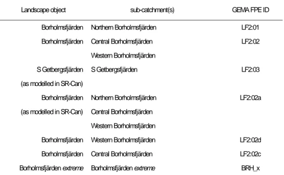
Table 3.1. GEMA discretisation of the Laxemar landscape objects shown in Figure 3.1. The GEMA flowpath elements identifiers for the different object interpretations are noted, these are used throughout this report.

Landscape object sub-catchment(s) GEMA FPE ID

Borholmsfjärden Northern Borholmsfjärden LF2:01

Borholmsfjärden Central Borholmsfjärden Western Borholmsfjärden

LF2:02

S Getbergsfjärden (as modelled in SR-Can)

S Getbergsfjärden LF2:03

Borholmsfjärden Northern Borholmsfjärden LF2:02a (as modelled in SR-Can) Central Borholmsfjärden

Western Borholmsfjärden

Borholmsfjärden Western Borholmsfjärden LF2:02d

Borholmsfjärden Central Borholmsfjärden LF2:02c

Borholmsfjärden extreme Borholmsfjärden extreme BRH_x

3.2 An evolving system: Basin Borholmsfjärden, Laxemar

3.2.1 Landscape features

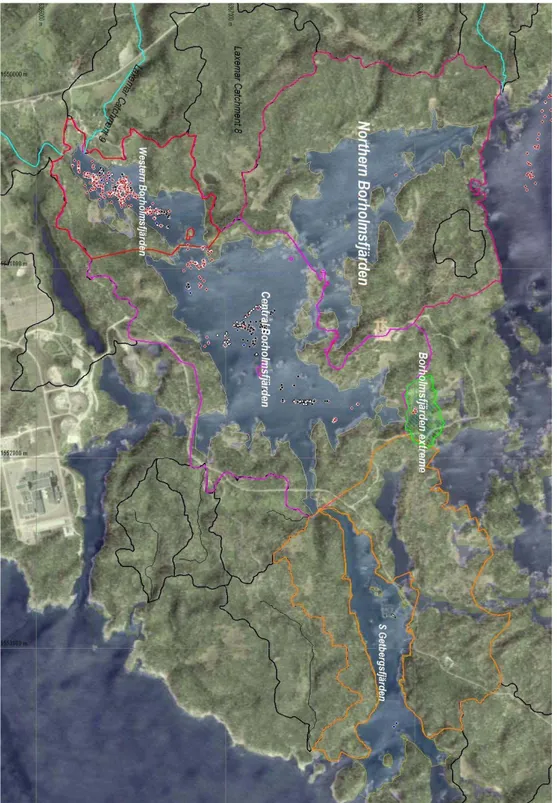
The GEMA models here describe the surface drainage system comprising two basins at the Laxemar candidate site: Borholmsfjärden and S Getbergsfjärden. Figure 3.1 is a map of the area based on the SKB topographic dataset for the Laxemar site

SDEADM.UMEU_SM_HOJ_2102 (Lindborg, 2006) provided by SKB. The release points calculated by SKB in SR-Can are also plotted to illustrate the parts of the surface drainage system that might receive input. Today the basins connect to the Baltic. In SR-Can (SKB, 2006a) Borholmsfjärden was modelled as a single object with S Getbergsfjärden as a second object downstream. As indicated in Figure 3.1 the GEMA interpretation recognises that basin Borholmsfjärden can be described by three sub-catchments. The Laxemar catchments (SKB datafile SDEADM.POS_SM_VTN_3286) is used for this purpose. However, catchments around coastal objects are not explicitly identified so the sub-catchments of Borholmsfjärden have been determined by a review of the topography. The interpretation of the objects is shown in Table 3.1.

Figure 3.1. Map of Laxemar in the present day showing drainage system from Laxemar catchments 8, 9 and 10. Coloured areas show the local catchments of the basins. In the GEMA discretisation of Basin Borholmsfjärden one, two or three distinct objects can be identified where SR-Can (SKB, 2006a) identifies just one. Northern Borholmsfjärden is the main focus since it has no inflow from upstream catchments. To the northeast of Bor-holmsfjärden is a smaller isolated catchment identified as BorBor-holmsfjärden extreme. Re-lease points are taken from SKB (2006a). Topographic map from SKB (Lindborg 2006)

with overlay image taken from GoogleEarth TM _{and fitted to the map using Global} Map-per (2007). (c) 5000 AD (a) 2000 AD (d) 900 0 AD (b) 300 0 AD

Figure 3.2. Four stages in the evolution of Laxemar’s bays. Land rise at 1 mm y-1 _{means 1}

m of elevation in 1000 years. Within the present day catchment areas the water bodies retreat and new soil emerges. By 5000 AD the whole of northern Borholmsfjärden is above sea level. Converted to an agricultural area, drainage will be by a stream network.

By 9000 AD all of Borholmsfjärden is a terrestrial system. Water bodies are shown in purple with the emergent land indicated by orange shading.

The interpretation of objects is important for the description of mass balance. Basin Bor-holmsfjärden is part of the larger Laxemar drainage system. Lindborg (2006) notes that Laxemar catchments 8, 9 and 10 discharge into Borholmsfjärden. By subdividing the ba-sin dilution is much less for some GEMA objects than for the whole of the bay. For ex-ample, the northern bay does not receive any drainage inflow. The potential for dilution in the water body is therefore much reduced compared to the overall objects. The north-ern basin (LF2:01) is the reference for the GEMA modelling. For this reason, the object identified as Borholmsfjärden extreme has also been modelled using GEMA, since it

could receives a contaminant discharge. Section 3.2.5 describes this area in greater detail.

3.2.2 Landscape evolution at Laxemar

Lindborg (2006) provides basic data for the site description. Of central importance is the local land uplift rate of 1 mm y-1_{. SR-Can evaluated releases upto 10 000 AD. In the}

GEMA interpretation evolution was implemented as a series of step changes occurring at each one thousand years starting from the landscape at 2000 AD. The emergent land is illustrated in Figure 3.2.

Land rise is an ongoing processes and succession provides a guide for interpreting the ecosystem types during site evolution. The terrestrial landscape in the present day indi-cates the kinds of ecosystems that will form as the Baltic retreats. Table 3.2 lists the inter-pretation of the objects. The general trend is that marine bays become isolated losing their salt content, to form freshwater lakes. Continued sedimentation and plant growth, com-bined with progressive falls in local sea level produce wetland areas.

During the evolution of bays to lakes and wetlands the emergent soils are rapidly colo-nised by terrestrial species. These soils are not managed and are designated here as “natu-ral soils”. Agricultu“natu-ral soils are assumed to be formed (by human action) as soon as local hydrological conditions allow, i.e., when the wetland area is above sea level. In the GEMA models here agricultural land areas are associated with streams which provide local drainage.

The description of land use types given by Lindborg (2006) gives more detail than the existing radionuclide database can accommodate. For this reason the interpretation of aquatic systems is limited to marine bay (brackish water), lake (freshwater), wetland (freshwater) and stream (see Section 3.4). The terrestrial systems are natural soils (coastal and terrestrial) and agricultural soils. Forests are also part of the system but these are known to be at the higher elevations. According to the release distribution shown in Figure 3.1, none of the existing forested areas are likely to become contaminated.

Figure 3.2 illustrates key features of the evolutionary sequence. In the 1000 years to 3000 AD northern Borholmsfjärden becomes a lake, isolated from the main body of the origi-nal bay. The western portion is still connected to the central water body but by 5000 AD both northern and western Borholmsfjärden are above sea level and are interpreted as ag-ricultural land, having passed though a wetland phase. Upto 9000 AD the water body in the central portion of Borholmsfjärden shrinks to a wetland until, it is assumed, it is drained for agricultural use.

Table 3.2. The sequence of ecosystems for the different system discretisations used in the GEMA interpretation of the Laxemar bays.

Flowpath elements - GEMA objects

date LF2:01 LF2:02 LF2:03 LF2:02a LF2:02d LF2:02c BRH_x

2000 AD BCS BCS BCS BCS BCS BCS LNS

3000 AD LNS LNS LNS LNS LNS LNS WNS

4000 AD WNS LNS LNS LNS WNS LNS SAS

5000 AD SAS WNS LNS WNS SAS WNS SAS

6000 AD SAS WNS LNS WNS SAS WNS SAS

7000 AD SAS WAS LNS WAS SAS WAS SAS

8000 AD SAS WAS LNS WAS SAS WAS SAS

9000 AD SAS SAS WNS SAS SAS SAS SAS

10000 AD SAS SAS WNS SAS SAS SAS SAS

key Aquatic Terrestrial BCS Bay Coastal / Natural soils

LNS Lake Natural soils

WNS Wetland Natural soils WAS Wetland Agricultural soils

SAS Streams Agricultural soils

0 m 6 m 12 m 0 m 6 m 12 m

Figure 3.3. Thickness of the QD in the model region. Sediment thickness in the bays is fairly constant at around 7.4 m in Borholmsfjärden. A high fraction of S Getbergsfjärden has similar thicknesses of sediment. The SR-Can release points indicate that the deep sediment of the water bodies lies above the discharge points.

The spatial discretisation directly effects how the objects are characterised. The reference area, LF2:01 (northern Borholmsfjärden), is assumed to be drained and converted to agri-cultural land at 5000 AD by which time the whole of the object is above sea level. Streams are then managed to provide the necessary drainage. In the case of the whole Borholmsfjärden object (LF2:02a, as interpreted by SKB as a single object) the area is not wholly above sea level until 9000 AD. Nevertheless large areas of relatively flat soils will already have emerged by 5000 AD. These may be interpreted as being available for agri-cultural production. The water body is shallow and is interpreted as wetland. For this system the ecosystem type is assumed to be Wetland with Agricultural soils. Agricultural soils are the most productive areas and more of the GEMA exposure pathways are active in such areas.

Lindborg (2006) notes that releases from bedrock are generally associated with low points in the topography. This is confirmed by the releases point shown in Figure 3.1. Lindborg (2006) also describes the thickness of the Quaternary deposits (datafile SDEADM.POS_SM_GEO_2653). The thickness map is shown in Figure 3.3.

The release points correspond to the paths taken by release from the individual canisters at the repository depth. In SR-Can, SKB assign an ensemble of releases to a particular

500 750 1000 1250

Distance along section [m]

-10 -8 -6 -4 -2 0 2 4 6 8 10 El evatio n [m ] Bedrock Sediment/ Quaternary deposits 2000 AD - sea level = 0 m 500 750 1000 1250

Distance along section [m]

-10 -8 -6 -4 -2 0 2 4 6 8 10 El evatio n [m ] Bedrock Sediment/ Quaternary deposits

3000 AD - sea level = -1 m Contaminated areas _{of "new" soil}

Figure 3.4. Cross section SW-NE across northern Borholmsfjärden (LF2:01) at 2000 and 3000 AD. The bedrock and thickness of Quaternary material are indicated illustrating that the present day terrestrial area would remain as uncontaminated catchment. Topography of bay shoreline for other objects is similar. Emergent soils are indicated.

ecosystem to the object in question, neglecting the spatial distribution of points within the object. Similarly in GEMA, releases enter the biosphere objects at the lowest points. In the Borholmsfjärden and Getbergsfjärden objects the releases are therefore to the bot-tom of the QD. During bay, lake and wetland phases this is interpreted as a release to deep sediment of the aquatic submodel. During agricultural phases it is assumed that the object is well drained and the QD differs from the deep sediment. The top sediment and deep sediment are therefore treated as smaller compartments in the stream’s hyporheic zone. Thus, release is to deep sediment unless the object is agricultural land in which case the release is to the QD. This interpretation is reflected in the assumed mass balance schemes for objects in the GEMA representations described in the following section.

3.2.3 Parameterisation of water and solid material balance: transfer coefficients

Equations (2.3) suggest contaminant transport in GEMA is modelled straightforwardly. The volumes of compartments and the internal characteristics are required and mass fluxes determine the contaminant flows. This section illustrates the procedure for deter-mining the fluxes in Equation (2.2).

Lindborg (2006) shows that the Borholmsfjärden – Getbergsfjärden drainage system is part of the flow system of three catchments, identified as Laxemar 8, 9 and 10. These enter the western part of Borholmsfjärden (see Figure 3.1). Laxemar 7 discharges to the north of Borholmsfjärden. Laxemar 8 is small (485481 m2_{) but Laxemar 9 and 10 are}

major catchments at Laxemar, (2755420 m2 _{and 47628017 m}2 _{respectively). Lindborg}

(2006) gives a range for precipitation and ETp in the Laxemar region. GEMA uses 0.6 m y-1 _{rainfall and 0.5 m y}-1 _{for ETp. These values, taken from Bergström and Barkefors}

(2004), lie within this range2_{. The discharge from the catchments entering the modelled}

system is then determined as

, (3.1)

(

)

where solid material entering the system is assumed to be driven by the suspended solid load in the bay/lake/stream. These flows enter objects connected to the upstream drainage system: LF2:02a for the whole of Borholmsfjärden, LF2:02 when northern

2 _{Precipitation at Laxemar is slightly higher (0.655 m y}-1_{) in SR-Can (SKB, 2006b) and}

combined evaporation and transpiration, in the forest model slightly lower (0.466 m y-1_{). These}

are based on single observations and as such are not necessarily representative of the long term average. At the time that the GEMA models were constructed the details of SR-Can had not been published. The earlier precipitation and ETp values were therefore used in the GEMA calculations. The effect of using the Sr-Can values is to decrease dose by around a factor of up to two for the poorly sorbing nuclides (36Cl, 129_{I) but much less for the members of the} 226_Ra

fjärden is treated independently or LF2:02d when three elements of Borholmsfjärden are assumed, see Table 3.1.

At the local level of each GEMA FPE the matrices for water and solid material fluxes are written explicitly. These take into account the interpretation of local hydrology. Figure 3.4 illustrates the typical situation in the modelled area. A SW-NE cut across northern Borholmsfjärden (LF2:01) shows the bedrock, QD and water column of the bay/lake at 2000 AD and 3000 AD. Activity enters the system from the bedrock below the QD. It is assumed that there is a small gradient driving water fluxes up through the sediment. SKB’s SR-Can interpretation is different but the assumption made here is that water flows though the QD, allowing time for contaminant retention which is then distributed throughout the sediment for inclusion in emergent soils as they form with the retreat of the water body. Starting from the situation at 2000 AD, contaminated parts of the system are restricted to the areas of sediment underlying the water body. The higher elevations are part of the local catchment but remain uncontaminated. Terrestrial soils only become contaminated as a result of the legacy contamination as the local water level falls. The higher parts of the system at 2000 AD all have thin QD layers and retain little water. Run off from these areas is assumed to be directly to the water body. As the waters re-treat, however, contaminated soils are formed from the sediments under the bay. Water balance is then assumed as shown in Figure 3.5 for the 3000 AD system. Drainage from the uncontaminated higher areas flows to the newly emerged soils where it is assumed to infiltrate and migrate to the water body. This assumption adds to the turnover (and mix-ing) in the QD and aquatic sediment layers of the model. The assumption reflects the relative lack of understanding of local hydrology.

There is a small water flux assumed at the bottom of the system, driven by the water flux from the bedrock with velocity vGBI (taken from SKB, 2006c). Otherwise precipitation and evapotranspiration account for the fluxes. Capillary rise is used to drive the flow from the QD to the top soil. The value is 0.1 m y-1 _{taken from Kłos et al. (1996).}

The corresponding solid material scheme is shown in Figure 3.6. For northern Borholms-fjärden the only solid input is from deposition. No details were available for this process so a small value of mdep = 0.01 kg m-2 _y-1 _{is assumed and this balances erosion with the}

same value.

As a conservative feature it is assumed that there is no solid flux downstream, cf. the in-put flux described by Equation (3.1). This manifests itself as net sedimentation in the system, denoted by the flux M_DSed_GBI in Figure 3.6. This flux is used to balance the system since the compartments are maintained constant throughout each 1000 year pe-riod. Although there is a mass flux here it is not assumed that radionuclides are included in this transfer. The whole of the accumulated inventory is then available for transfer to land during the next evolutionary step.

Some of the solid fluxes assume suspended solid fluxes with the water flow, using the suspended solid load in the compartments i, αi kg m-3. This value is taken from Kłos et al.

(1996). The other major flux is bioturbation as modelled by Kłos et al. (1996).

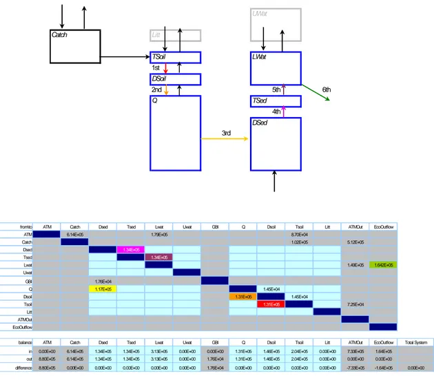
The transfer matrix for 210_{Po in the northern Borholmsfjärden lake at 3000 AD is shown}

in Figure 3.7. The values are calculated using Equations (2.3) together with the water and solid material fluxes in Figures 3.5 and 3.6.

UWat Catch Litt TSoil LWat 1st DSoil 2nd 5th 6th Q TSed 4th DSed 3rd

from\to ATM Catch Dsed Tsed Lwat Uwat GBI Q Dsoil Tsoil Litt ATMOut EcoOutflow

ATM 6.14E+05 1.79E+05 8.70E+04

Catch 1.02E+05 5.12E+05

Dsed 1.34E+05

Tsed 1.34E+05

Lwat 1.49E+05 1.642E+05

Uwat

GBI 1.76E+04

Q 1.17E+05 1.45E+04

Dsoil 1.31E+05 1.45E+04

Tsoil 1.31E+05 7.25E+04

Litt ATMOut EcoOutflow

balance ATM Catch Dsed Tsed Lwat Uwat GBI Q Dsoil Tsoil Litt ATMOut EcoOutflow Total System in 0.00E+00 6.14E+05 1.34E+05 1.34E+05 3.13E+05 0.00E+00 0.00E+00 1.31E+05 1.46E+05 2.04E+05 0.00E+00 7.33E+05 1.64E+05

out 8.80E+05 6.14E+05 1.34E+05 1.34E+05 3.13E+05 0.00E+00 1.76E+04 1.31E+05 1.46E+05 2.04E+05 0.00E+00 0.00E+00 0.00E+00 difference 8.80E+05 0.00E+00 0.00E+00 0.00E+00 0.00E+00 0.00E+00 1.76E+04 0.00E+00 0.00E+00 0.00E+00 0.00E+00 -7.33E+05 -1.64E+05 0.00E+00

F_inflow_i = 0 For all i F_ATM_Catch = 6.14E+05 = dppt*ACatch F_ATM_Lwat = 1.79E+05 = dppt*ALWat F_ATM_Tsoil = 8.70E+04 = dppt*ATsoil

F_Catch_Tsoil = 1.02E+05 = F_ATM_Catch-F_Catch_ATMOut F_Catch_ATMOut = 5.12E+05 = dETp*ACatch

F_Dsed_Tsed = 1.34E+05 = F_GBI_Dsed+F_Q_Dsed F_Tsed_Lwat = 1.34E+05 = F_Dsed_Tsed F_Lwat_ATMOut = 1.49E+05 = dETp*ALWat

F_Lwat_EcoOutflow = 1.64E+05 = F_ATM_Lwat+F_Tsed_Lwat-F_Lwat_ATMOut F_GBI_Dsed = 1.76E+04 = ADSed*vGBI*SIN(phiGBI)

F_Q_Dsed = 1.17E+05 = F_Dsoil_Q-F_Q_Dsoil+F_GBI_Q F_Q_Dsoil = 1.45E+04 = dcapil*AQ

F_Dsoil_Q = 1.31E+05 = F_Q_Dsoil+F_Tsoil_Dsoil-F_Dsoil_Tsoil F_Dsoil_Tsoil = 1.45E+04 = dcapil*ADSoil

F_Tsoil_Dsoil = 1.31E+05 = F_ATM_Tsoil+F_Catch_Tsoil+F_Dsoil_Tsoil-F_Tsoil_ATMOut F_Tsoil_ATMOut = 7.25E+04 = dETTSoil*ATsoil

Figure 3.5. Water balance for northern Borholmsfjärden at 3000 AD. A glossary of GEMA parameters is given in Appendix D.

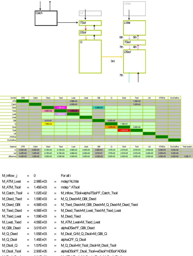
UWat Catch Litt TSoil LWat DSoil 6th 5th Q T 7th 4th DSed 3rd 7th Sed

from\to ATM Catch Dsed Tsed Lwat Uwat GBI Q Dsoil Tsoil Litt ATMOut EcoOutflow

ATM 2.98E+03 1.45E+03

Catch 0.00E+00 1.02E+02

Dsed 1.59E+03 4.56E+03

Tsed 4.56E+03 1.59E+03

Lwat 4.56E+03

Uwat

GBI 3.51E+01 0.00E+00

Q 1.55E+03 1.45E+01

Dsoil 1.57E+03 2.90E+05

Tsoil 2.91E+05

Litt ATMOut EcoOutflow

balance ATM Catch Dsed Tsed Lwat Uwat GBI Q Dsoil Tsoil Litt ATMOut EcoOutflow Total system in 0.00E+00 0.00E+00 6.15E+03 6.15E+03 4.56E+03 0.00E+00 4.56E+03 1.57E+03 2.91E+05 2.91E+05 0.00E+00 0.00E+00 0.00E+00 out 4.43E+03 1.02E+02 6.15E+03 6.15E+03 4.56E+03 0.00E+00 3.51E+01 1.57E+03 2.91E+05 2.91E+05 0.00E+00 0.00E+00 0.00E+00 difference 4.43E+03 1.02E+02 0.00E+00 0.00E+00 0.00E+00 0.00E+00 -4.53E+03 0.00E+00 0.00E+00 0.00E+00 0.00E+00 0.00E+00 0.00E+00 1.00E-11

M_inflow _j = 0 For all i M_ATM_Lwat = 2.98E+03 = mdep*ALWat M_ATM_Tsoil = 1.45E+03 = mdep * ATsoil

M_Catch_Tsoil = 1.02E+02 = M_inflow_TSoil+alphaTSoil*F_Catch_Tsoil M_Dsed_Tsed = 1.59E+03 = M_Q_Dsed+M_GBI_Dsed

M_Dsed_GBI = 4.56E+03 = M_Tsed_Dsed+M_GBI_Dsed+M_Q_Dsed-M_Dsed_Tsed M_Tsed_Dsed = 4.56E+03 = M_Dsed_Tsed+M_Lwat_Tsed-M_Tsed_Lwat

M_Tsed_Lwat = 1.59E+03 = M_Dsed_Tsed

M_Lwat_Tsed = 4.56E+03 = M_ATM_Lwat+M_Tsed_Lwat M_GBI_Dsed = 3.51E+01 = alphaDSed*F_GBI_Dsed M_Q_Dsed = 1.55E+03 = M_Dsoil_Q-M_Q_Dsoil+M_GBI_Q M_Q_Dsoil = 1.45E+01 = alphaQ*F_Q_Dsoil

M_Dsoil_Q = 1.57E+03 = M_Q_Dsoil+M_Tsoil_Dsoil-M_Dsoil_Tsoil M_Dsoil_Tsoil = 2.90E+05 = alphaDSoil*F_Dsoil_Tsoil+wDsoil*mDSoil*ADSoil M_Tsoil_Dsoil = 2.91E+05 = M_ATM_Tsoil+M_Catch_Tsoil+M_Dsoil_Tsoil

Figure 3.6. Solid material flux balance for northern Borholmsfjärden at 3000 AD. A glossary of GEMA parameters is given in Appendix D.

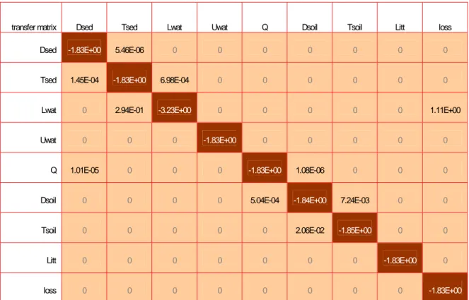
transfer matrix Dsed Tsed Lwat Uwat Q Dsoil Tsoil Litt loss

Dsed -1.83E+00 5.46E-06 0 0 0 0 0 0 0

Tsed 1.45E-04 -1.83E+00 6.98E-04 0 0 0 0 0 0

Lwat 0 2.94E-01 -3.23E+00 0 0 0 0 0 1.11E+00

Uwat 0 0 0 -1.83E+00 0 0 0 0 0

Q 1.01E-05 0 0 0 -1.83E+00 1.08E-06 0 0 0

Dsoil 0 0 0 0 5.04E-04 -1.84E+00 7.24E-03 0 0

Tsoil 0 0 0 0 0 2.06E-02 -1.85E+00 0 0

Litt 0 0 0 0 0 0 0 -1.83E+00 0

0 0 0 0 0 0

loss 0 0 -1.83E+00

Figure 3.7. GEMA transfer coefficients for 210_{Po in the representation of northern}

Borholmsfjärden at 3000 AD. The values are calculated from QD, soils, sediments

(

)

using the water and solid material fluxes of Figures 3.5 and 3.6 respectively combined with the following compartment kd values (Table 3.7):

KLitt Not used m 3 _kg-1

KTSoil 0.5 m 3 _kg-1

KDSoil 7 m 3 _kg-1

KQ 7 m 3 _kg-1

KUWat Not used m 3 kg-1

KLWat 10 m 3 _kg-1

KTSed 7 m 3 _kg-1

KDSed 7 m 3 _kg-1

lambda0 1.83E+00 y-1

Time invariant compartment properties are given in Table 3.3 and the time varying parameters in Table 3.4. The leading diagonal of the matrix represents the sum of all losses (negative) from the compartment, including radioactive decay at the rate deter-mined by the decay constant lambda0.

UWat Catch Litt TSoil LWat 1st DSoil 2nd 5th 6th Q TSed 4th DSed 3rd

F_ATM_Catch = dppt*ACatch = 6.14E+05

F_ATM_Lwat = dppt*ALWat = 1.33E+02

F_ATM_Tsoil = dppt*ATsoil = 2.65E+05

F_Catch_Tsoil = F_ATM_Catch-F_Catch_ATMOut = 1.02E+05

F_Catch_ATMOut = dETp*ACatch = 5.12E+05

F_Dsed_Tsed = F_GBI_Dsed+F_Q_Dsed = 1.73E+05

F_Tsed_Lwat = F_Dsed_Tsed = 1.73E+05

F_Lwat_ATMOut = dETp*ALWat = 1.11E+02

F_Lwat_EcoOutflow = F_ATM_Lwat+F_Tsed_Lwat-F_Lwat_ATMOut = 1.73E+05

F_GBI_Q = AQ*vGBI*SIN(phiGBI) = 2.61E+04

F_Q_Dsed = F_Dsoil_Q-F_Q_Dsoil+F_GBI_Q = 1.73E+05

F_Q_Dsoil = dcapil*AQ = 4.42E+04

F_Dsoil_Q = F_Q_Dsoil+F_Tsoil_Dsoil-F_Dsoil_Tsoil = 1.91E+05

F_Dsoil_Tsoil = dcapil*ADSoil = 4.42E+04

F_Tsoil_Dsoil = F_ATM_Tsoil+F_Catch_Tsoil+F_Dsoil_Tsoil-F_Tsoil_ATMOut = 1.91E+05

F_Tsoil_ATMOut = dETTSoil*ATsoil = 2.21E+05

UWat Catch Litt TSoil LWat DSoil 6th 5th Q TSed 4th DSed 3rd

M_ATM_Lwat = mdep*ALWat = 2.22E+00

M_ATM_Tsoil = mdep * ATsoil = 4.42E+03

M_Catch_Tsoil = M_inflow_TSoil+alphaTSoil*F_Catch_Tsoil = 1.02E+02

M_Dsed_Tsed = M_Q_Dsed+M_GBI_Dsed = 4.55E+03

M_Tsed_Lwat = M_Dsed_Tsed = 4.55E+03

M_Lwat_EcoOutflow = M_Tsed_Lwat+M_ATM_Lwat+M_Catch_Lwat = 4.55E+03

M_GBI_Q = alphaQ*F_GBI_Q = 2.61E+01

M_Q_Dsed = M_Dsoil_Q-M_Q_Dsoil+M_GBI_Q = 4.55E+03

M_Q_Dsoil = alphaQ*F_Q_Dsoil = 4.42E+01

M_Dsoil_Q = M_Q_Dsoil+M_Tsoil_Dsoil-M_Dsoil_Tsoil = 4.57E+03 M_Dsoil_Tsoil = alphaDSoil*F_Dsoil_Tsoil+wDsoil*mDSoil*ADSoil = 8.85E+05 M_Tsoil_Dsoil = M_ATM_Tsoil+M_Catch_Tsoil+M_Dsoil_Tsoil = 8.89E+05

Figure 3.8. Water and solid material flux balance for the representation of agricultural soils with streams. Numerical values for northern Borholmsfjärden (LF2:01) at 5000 AD.

transfer matrix Dsed Tsed Lwat Uwat Q Dsoil Tsoil Litt loss

Dsed -2.18E+00 3.55E-01 0 0 0 0 0 0 0

Tsed 0 -3.07E+00 1.24E+00 0 0 0 0 0 0

Lwat 0 0 -4.92E+03 0 0 0 0 0 4.92E+03

Uwat 0 0 0 -1.83E+00 0 0 0 0 0

Q 5.57E-06 0 0 0 -1.83E+00 1.21E-06 0 0 0

Dsoil 0 0 0 0 7.76E-05 -1.83E+00 2.17E-03 0 0

Tsoil 0 0 0 0 0 1.80E-02 -1.85E+00 0 0

Litt 0 0 0 0 0 0 0 -1.83E+00 0

0 0 0 0 0 0

loss 0 0 -1.83E+00

Figure 3.9. GEMA transfer coefficients for 210_{Po in the representation of northern}

Borholmsfjärden as agricultural land from 5000 to 10 000 AD. The values are calculated from QD, soils, sediments

(

)

using the water and solid material fluxes of Figure 3.8 respectively combined with the following compartment kd values (Table 3.7):

KLitt Not used m 3 _kg-1

KTSoil 0.5 m 3 _kg-1

KDSoil 7 m 3 _kg-1

KQ 7 m 3 _kg-1

KUWat Not used m 3 kg-1

KLWat 10 m 3 _kg-1

KTSed 7 m 3 _kg-1

KDSed 7 m 3 _kg-1

lambda0 1.83E+00 y-1

Time invariant compartment properties are given in Table 3.3 and the time varying parameters in Table 3.4. The leading diagonal of the matrix represents the sum of all losses (negative) from the compartment, including radioactive decay at the rate determined by the decay constant lambda0.

Table 3.3. Time invariant parameters for LF2:01. These parameters are applicable to all ecosystem at all times.

Parameter units value source

evapotranspiration dETp m y-1 0.5 Bergström & Barkefors (2004) precipitation dppt m y-1 0.6 Bergström & Barkefors (2004)

mass deposition rate mDep kg m-2 y-₁ 0.01 Assumed value

erosion rate mEros kg m-2 y-₁ 0.01 Assumed value

vGBI m y-1 0.058 SKB (2006c)

groundwater velocity entering

biosphere _{phiGBI rad 1.570796 Assumed vertical}

capillary rise dcapil m y-1 0.1 Klos et al (1996)

active biomass mDSoil kg m-2 0.1 Klos et al (1996)

biomass activity wDSoil y-1 20 Klos et al (1996)

irrigation dirri m y-1 0 No irrigation

suspended solid load alphaDSed kg m-3 0.002 Assumed from Klos et al. (1996) alphaTSed kg m-3 0.002 Assumed from Klos et al. (1996) alphaLWat kg m-3 0.002 Assumed from Klos et al. (1996)

alphaUWat kg m-3 not used

alphaQ kg m-3 0.001 Assumed from Klos et al. (1996) alphaDSoil kg m-3 0.001 Assumed from Klos et al. (1996) alphaTSoil kg m-3 0.001 Assumed from Klos et al. (1996)

alphaLitt kg m-3 not used

compartment density* RhoLWat kg m-3 1000

RhoDSed kg m-3 2650 Density of parent mineral

RhoTSed kg m-3 2650

RhoQ kg m-3 2650

RhoDSoil kg m-3 2650

RhoTSoil kg m-3 2650

RhoLitt kg m-3 2650

* There is some debate about the use of density in the SR-Can models. The use of mineral density here means that bulk density can be readily expressed as

(

)

bulk ε ρ

ρ = 1−

if the sample is dried. For a wet sample this might become

(

)

bulk ε ρ θρ

ρ = 1− +

The schematic water flux system in Figure 3.5 is valid for evolving bays, lakes and wet-lands. There are difference in the representation of agricultural land. The compartments differ in size but primarily the stream carries suspended sediment load downstream. The mass balance scheme for agricultural land is shown in Figure 3.8. The structure is representative of other SAS ecosystems. In the case of WAS (see Table 3.2) the schemes shown in Figures 3.5 and 3.6 apply. The transfer matrix for 210_{Po is shown in Figure 3.9}

Many of the parameters in the model are not assumed to change in time. These are listed in Table 3.3. Details for the northern Borholmsfjärden system are given in Appendix E. Details of the other GEMA models are available from the author on request.

3.2.4 Time varying parameters

Volumes and areas change in time and these influence the water and solid material fluxes through the relations listed in Figures 3.5, 3.6 and 3.7. Using a step change regime to model system change means that the shape of the landscape objects illustrated in Figure 3.2 can be used to define the objects. Global Mapper (2007) has been used for this pur-pose. The procedure is as follows:

1. Determine the shape of the object based on the contour line at intervals defined by sea level fall each one thousand years (0 m, present day, -1 m 3000 AD, -2 m 4000 AD, etc.). GlobalMapper (2007) calculates the area within the current sea level contour.

2. The area of the emergent soil at each evolutionary stage is calculated from the difference of aquatic areas.

3. The volume of the water body is also determined by routines in GlobalMapper. Together with the area data, the depth of the water column is determined. Bergström et al. (1999) is the source for the soil thicknesses and the depth of compart-ment Q is the difference in the thickness of the overall QD from the QD map and the deep and top soil depths. Bay, lake and wetland sediments are assumed to have a top sediment of 0.1 m, consistent with the data in Lindborg (2006). Streams are assumed to be 2 m wide and 20 cm deep based on observations of the model area. The depth of the top sedi-ment is also 0.1 m and the deep sedisedi-ment of streams is 0.2 m above the QD compartsedi-ment. Characteristics of the soil are taken from Bergström et al. (1999) in terms of porosity. The degree of saturation is assumed. Details for northern Borholmsfjärden are summarised in Table 3.4.

Contaminant transport in the GEMA model is governed by the expression in Equation (2.1). The step change approach to evolution runs the model for each evolutionary system description and then changes the parameters to reflect the new state. There is a need to transfer activity between the compartments as a result of the evolutionary changes. Figure 3.4 illustrates the situation.

The bed sediment of the lake at 2000 AD accumulates activity. By 3000 AD some of the sediment now underlies soil: there is a net transfer from aquatic sediment to terrestrial soils and QD. In the SR-Can review this transfer is modelled using a transfer matrix T in the form