Some approaches to car demand modelling

Some approaches to car

demand modelling

by IanOwen Idnsson

and Dan Shneerson

Some approaches to car

demand modelling

by Ian Owen Iansson

1.1 1.2 2.1 2.1.1 2.1.2 2.2 2.2.1 2.2.2 2.2.3 2.2.3.1 2.2.3.2 2.2.3.3 2.3 2.3.1 2.3.1.1 2.3.2 2.3.2.1 2.4 2.4.1 ABSTRACT INTRODUCTION

General remarks on theory and practice of demand estimation in economics

Characteristics of car demand, and different purposes 3

of car demand studies

MODELS FOR ESTIMATING "GROWTH CURVES" FOR CAR OWNERSHIP

The epidemic diffusion theory

The forecasting model of the Swedish National Road Administration

Explaining the past vs. forecasting the future

both diffusion and econo

Models allowing for

mic factors

Distinguishing the diffusion and income effects TRRL models

Bonus' work

Behaviour of quasi Engel curves over time Vertical and horizontal diffusion

The shape of the aggregate growth curve

Evidence of diffusion and income effects in Sweden in the 19705

Quasi Engel curves for different life cycle categories 1974-1978

Two categories of special importance (l) first car

ownership of retired people; (2) second-car ownership of

married couples

Income-elasticity estimation on cross-section data

Problems of testing cross-section estimates on time series data

Long-term forecasting: the issue of the saturation level Stationary equilibrium of car ownership vs. the satura tion level

VTI RAPPORT 251A

10 IO 11 12 13 15 16 17 l8 19 19 23 23 25 28 28

3.1 3.2 3.3 3.3.1 3.3.1.1 3.3.1.2 3.3.2 3.3.3 3.3.4 4.1 4.2 4.3 4.4 4.4.1 4.4.2 4.4.2.1 4.5

MODELS WITH A VIEW TO EXPLAINING FLUCTUA-TIONS IN CAR PURCHASES

The change in focus from car stock to car investment flow

A static model Dynamic models

The basic stock-adjustment model Rental cost vs. purchase price of cars

Credit terms and financial position of households Expectations

Car scrapping

Criticism of the stock-adjustment model

SOCIO-ECONOMIC STUDIES OF HOUSEHOLD CAR OWNERSHIP AND USE

Historical background

Some questions of the socio-economic factors of car ownership

"Carlessness" in Sweden and the USA: some basic findings from recent travel surveys

Models of household car ownership and use Modal choice, given car ownership

Car ownership

An example of a disaggregate model of car ownership Limitations of cross-section analysis in respect of ex-plaining/forecasting demand development over time CONCLUDING REMARKS

REFERENCES

VTI RAPPORT 251A

36

36

4o

42

43

45

46

47

50

53

56 56 57 58 65 66 67 68 72 76 77

by JanOwen Jansson and Dan Shneerson

National Swedish Road and Traffic Research Institute (VTI)

5-581 01 Linkoping, Sweden

ABSTRACT

A number of different approaches to car demand modelling can be found

in more or less separate literatures. There is work often sponsored by

the National Road Administration or other authorities responsible for road investment planning - with an ultimate view to forecasting the long-term development of car traffic. These models usually consist of two separate parts one for estimating the future level of car ownership, and another for estimating the average mileage per car.

For the purpose of fiscal and/or monetary stabilization policy, macro-economic models for short-term forecasting are developed. An import-ant and notoriously unpredictable item of total demand is private

investment by firms as well as by households in consumer durables.

Among the latter, cars is a major item. Fluctuations in total car

purchases from one year to another of t 30 96 are not unusual, and quite different models (than the models for forecasting the long-term develop-ment of car ownership) are used for predicting expenditure on cars 1-3

years hence.

As a natural extension of modal split modelling efforts, discrete choice models estimated on disaggregate cross-section data have been applied also for explaining car ownership. By this approach deeper knowledge of the socio-economic factors of importance for household car ownership has been obtained. The influence of local conditions like public transport supply and parking facilities on car ownership also become more tract-able by the disaggregate approach. On the other hand, some important factors for the long-term development of car demand like the price-elasticity and the diffusion process seem difficult to estimate by cross-section analysis only.

1.1 General remarks on theory and practice of demand estimation in

economics

A demand function the relationship between the quantity demanded of

a particular commodity or product in a particular period of time and the arguments determining the quantity demanded ("the explanatory

vari-ables") can be written quite generally:

D: f(P9P,an9myM9N919T)

D = quantity demanded of a particular product,

p 2 price of the product,

P : vector of prices of substitutes and complementary products, q = quality of the product,

Q = vector of qualities of substitutes and complementary products, m = marketing efforts for selling the product,

M : vector of marketing efforts for selling substitutes and

complemen-tary products,

N 2 population vector,

I : vector of incomes per head of different consumer categories, T = "taste" index

From the point of view of the producer of the product in question, two types or arguments can be distinguished: the small letter arguments, p, q, m, which represents control variables of the producer, and the capitals

P, Q, M, N, I, T, which are out of the control of the producer of the

product in question. Two types of questions which the demand function may help to answer then suggest themselves:

1. Marketing poliCy: What will the effect on D be of changes in price, quality, and various selling efforts on the part of the producer?

2. Demand forecasting: If the producer stays put, i.e. given the values of p, q, and m, how will D develop in the future?

markets occur when competitors can be expected to react to changes in price p (i.e. p and P are somehow interrelated). The effect on demand

of quality changes is a neglected matter in economic theory. The

traditional way of dealing with quality is to define the concept w: a change in quality of a product is regarded as the appearance of a new product, and the theory is concerned only with price and quantity

relationships own-price- and cross price-elasticities of demand.

Growing dissatisfaction with the neglect of quality in the theory of demand has been noticeable in the economic literature in the last decade. The best known contribution towards rectifying this neglect is Lancaster's "New approach to consumer theory" (Journal of Political

Economy, l966)*. The inpact of this new approach on general theory

has not been great so far. However, it should be mentioned that a modern school of thought in the special field of travel demand is allegedly based on Lancaster's theory.

The effect on demand of selling activities like advertising can be very

significant, but is notoriously difficult to quantify. Some people seem to

think that consumers can be manipulated at will by big business. Others (notably the businessmen themselves) mean that a bad product cannot be sold no matter how muchis put into sales promotion. There is no doubt,

however, that marketing in general, and advertising in particular are

professions in which skill is highly rewarded. To sell a product is an art rather than a science, which does not easily lend itself to the kind of quantifiable generalisations that economic theory is aiming at.

Demand forecasting is, in principle, a two stage exercise. First the

relationship between D and the arguments in the demand function, which the producer/seller of the product concerned cannot control, has to be estimated. Then the values of these arguments at given dates in the future have to be forecasted. The normal division of labour is that the models for demand forecasting of particular products are directly

* This was followed up by a book, namely K. Lancaster: Consumer

Demand: A New Approach. New York, 1971. VTI RAPPORT 251A

demand, one normally relies on the "official" ones made by national

agencies like the central statistical bureau.

Another general characteristic of demand forecasting models is that they are applicable to the industry level rather than to the individual firm level. In other words: The model aims at forecasting the size of the total market in the first place. Another, separate task is then to estimate the market shares of individual products within the interrelated

group of products concerned. On the industry level each of the vector

arguments P, Q, and M cancel out to a large extent. Individual product differentiation as well as changes in marketing and pricing policy of individual firms have primarily effects on market shares. On the other hand, if it can be expected that the average price will secularly rise or fall, or if a general tendency of quality improvement can be foreseen, total market size is likely to be affected, too. However, in general it is true to say that demand forecasting models are focusing on the effect of the demand of a particular product, of changes in population, income per head, and possibly taste.

The latter source of influence on demand is obviously as difficult to grasp as it is potentially important. Economists are inclined to assume

that "tastes are given" in demand modelling, simply because there is no ready way of predicting changes in taste.

In one important case, however, one has to face the fact that tastes do not stay constant. There is plenty of evidence that taste for a new product behaves in a fairly similar and regular manner. When a com-pletely new product is introduced, the "equilibrium level" of demand is normally not reached until a rather long period of "diffusion" has passed: that is to say, the strength of preferences for a new product seems to be steadily growing as a result of a learning process, which may last for a generation, or even longer. A lot of modelling efforts have been devoted to the estimation of "growth curves" for new products, from hybrid corn

to automobiles, on the basis of different theories of the nature of

diffusion.

A large number of studies of car demand exists in the economic

literature, not only empirical work, but also a substantial body of

theoretical and methodological discussion. The question is: what is so special with cars, explaining the great interest of economists?

An obious fact explaining a great deal of the interest shown in car demand modelling is that expenditures on cars constitute a considerable proportion in total household expenditures. Except for housing, no single item in the household budget matches the car expenditure. Another well known fact is that the whole life of people, and character of society have changed as a result of general car ownership; the other side of the coin being that the carless become something of an outcaste.

From a model-technical point of view, certain characteristics of

cars justify special treatment of problems of demand function estimation,

cars are durable goods with economic lives of 10-20 years,

the car is a comparatively new product, at least in some parts of the world, and it is arguable that the learning process is still going on, expenditures on cars are divisible between capital costs and operating costs, which both are significant items in household budgets; demand for car ownership and demand for car use are therefore each

import-ant in its own right.

_-The latter feature is not typical of most other durable goods like

refrigerators, washing-mashines, TV:s, etc., and it can be anticipated

that existing models of car demand still leave a lot to be desired regarding integration of the ownership and use aspects.

Of greater importance for understanding the different approaches to car demand modelling is, however, the different purposes. The motives of the bulk of studies of demand for cars can be classified into: (a) long-term forecasting of the level of car ownership and car traffic (b)

short-term forecasting of car purchases and car expenditure, (c) description of

the socio-economic factors of household car ownership. Most models of

number of kilometres travelled by car. This is done in two stages. First, the future number of cars is calculated, and in the second stage the average number of kilometres per car per year.

For the purpose of macro-economic stabilization policy, good predictions of the development 1-3 years hence of aggregate expenditure 'on

consumer durables, among which automobiles is a major item, are very

essential ingredients. The short-term fluctuations in consumer durable

investments constitute a great problem comparable to the more

notorious problem of the irregular pattern of investments by firms. Quite different models have been developed for the purpose of short-term forecasting than for long-term forecasting of the growth of car owner-ship.

In most countries nation-wide studies of household data concerning travel habits and car ownership are undertaken with regular intervals. These surveys form the basis for combined sociological and economic inquiries into the quality of life of different strata of the population with

respect to personal mobility, accessibility to essential services, etc., as

well as consequences of car ownership and use for family budgets. We

call for short such work, not wholly pertinently, socio-economic studies of household car ownership. The purpose of these studies is basically purely descriptive. However, latterly discrete choice models have been applied to disaggregate data of the socio-economic conditions of house holds with a particular view to predicting the effect on car ownership and use of transport policy variables like public transport price and quality.

In the following three chapters we will present and discuss in turn (i) models for estimating "growth curves" for car ownership, (ii) models with

a view to explaining fluctuations in car purchases, and (iii)

socio-economic studies of household car ownership.

individual car manufacturers, the most crucial aspect of car demand is that of market shares. How much make A will sell next year is more than anything else a matter of how that make is perceived by car buyers relative to makes B .... ..Z. The problem of the influence of quality on demand, and the choice between different types of cars are not dealt with in this study.

2.1 The epidemic diffusion theory

The introduction of the motor car was a transport innovation that has drastically changed the shape of society. It is only to be expected that no immediate acceptance and adoption of the car by all would occur. Rather a period of introduction is required during which the potential utility derived from cars will be realized in a process of changing habits as to

travel and travel intensive activities.

In analogy with the observed development of other relatively new pro ducts, one has sought to explain the growth of the total car fleet by a

theory of diffusion processes borrowed from biology and medicine. Car

ownership may be compared to an epidemic spreading at the rate of

contacts between those who carry the desease and those still uninfected.

To begin with the number of infected people will grow strictly expo-nentially, i.e. Nt : Noert where Nt is the total number of infected people

at time t, if NO is the initial number, and r is the "contact rate".

However, the proportion of inconsequential contacts between already infected people will gradually increase, which will slow down the diffusion process. As the position is approached where the whole population are infected, the growth curve is obviously markedly decelerating. A theory with the purpose of grasping the whole course of the epidemic has consequently to take into account that the growth curve has both an acceleration and a deceleration stage, and that the total population sets an upper limit to its growth.

By pursuing the aforementioned probability theoretical reasoning concern-ing contacts between infected and uninfected people, the followconcern-ing formula comes out as the first suggestion, and it has also been widely used

for statistical estimation:

Nmax : given total population (i.e. the maximum number of infected people)

" -N

k = max 0

N : ratio of the number of uninfected pe0ple to

the nur hber of infected people at the initial time

r = rate of contacts between each infected individual and unin-fected ones

t = chronological time

This function has a symmetrical S-shape; it is accelerating up to a level

where N t = 1/2 Nmax. At this level it has an inflexion-point, and is then

decelerating, going towards lm

_ax

as t goes to infinity.

The question is whether the diffusion process represented by the above formula is a good analogy to the course of develOpment of demand for a new product like the motor car? It is temptingly close to hand to think so from looking at the deve10pment of car ownership so far. See for example the graph for Sweden of the years l923-l980*. A sigmoid shape of the curve is quite suggestive here like in a number of other countries. Many observers have taken for granted that the car ownership growth curve is a typical reflection of a diffusion process for a new product.

* Two peculiarities of the car ownership figures plotted in figure 1

should be explained. From 1957 on there are two observations per

year. The higher figure is obtained by taking last year's stock of

cars, and adding cars registered in the current year, and deducting

cars deregistered because of scrappage. The lower figure

corre-sponds to the total number of cars registered as "active" the lst of

January each year. Since an increasing number of cars are

temporarily deregistered (but presumably not scrapped) this figure

falls short of the aforementioned figure. In 1972 there are three

figures plotted. In this year a procedure of "administrative

deregis-tration" started to be applied: cars that had been temporarily

deregistered for three years or more were definitely cancelled from the car register. The middle figure in 1972 corresponds to the total number after this additional deduction hasbeen made.

VTI RAPPORT 251A CA R OW NE RS HI P

0,4

4

Q3

-Fi gur e 1 o to ta ] num be r of pa ss en ge r ca rs on re gi st er at th e en d of ea ch ye ar x to ta i num be r of pa ss en ge r ca rs in ac ti ve us e at th e en d of ea ch ye ar x, xxxxxxxxx xxxxxx U ' U f i i U U T T I I I I I I I U U ' I ' U I ' I ' U I ' I I I ' I ' I ' f I I I I I I I I U I I ' U I I ' I

19

25

30

35

40

45

'

SO

55

60

65

70

75

80

Ca r own er sh ip gr owt hin Swe de n 19 23 -1 98 0.

2.1.1

2.1.2

The earliest version of car ownership growth models based on the epidemic diffusion theory is the same as (1) above, except that Nmax is

not 100 % of the population, but substantially less about half the

population can be assumed to be "immune" against car ownership for ever. Moreover, to make it independent of the population growth, both sides of the equation is divided by total population so that the dependant variable becomes "cars per person".

The forecasting model of the Swedish National Road Administration

A development of the simple epidemic diffusion approach has been made in the traffic forecasting model of the Swedish National Road Administra-tion in that separate car ownership growth curves are estimated for

different "life-cycle" categories. This means, first, that the dependant

variabel cars per person is replaced by cars per household, and secondly, that households are classified by age group, marital status, and whether or not they have children. For each type of household an individual growth curve is estimated: the saturation level is guestimated, and the best fit to that and to historical data of an epidemic diffusion curve is found in each

case.*

From the point of view of statistically testing the epidemic diffusion hypothesis, a problem is that not even in the United States the growth curve for car ownership can undeniably be said to have reached its saturation level. There is consequently no completed growth curve lending itself to scientific study, making it possible to test the basic theory of the

course of demand from introduction to saturation.

Explaining the past vs. forecasting the future.

The curve-fitting actually made regarding the development of car owner-ship has mostly been a sort of mixture of straightforward least square regression analysis of time-series data, and less strict extrapolation, disciplined though by forced adherence to a predetermined saturation

level.

* See Statens Vagverk: Personbilstrafiken 1 1980-2000.

P 0121980-12-29 Sverige

2.2

The idea is basically that besides the actual observations of car ownership in the past, there is another bench-mark that should not be ignored in the regression analysis, namely the saturation level. On the other hand, it is an unquestionable danger for the analysis of the past in constraining the

curve-fitting by a saturation level, which is strictly unknown.

In our view, it is useful to make a sharp distinction between the purpose of explaining the development in the past, and forecasting the future development of car ownership.In the following discussion we will first, (and extensively) deal with the problem of explaining the past, actually observed development. As a separate question we will then take up the problem of predicting the future. In the latter connection the issue of the saturation level has its right place.

Models allowing for both diffusion and economic factors.

The car ownership growth curve has been observed in a steadily growing economy. So how can we know that car ownership growth is not simply a result of rising income? At least, we think it is very unlikely that the car

ownership growth observed so far is wholly explained by diffusion by the

"demonstration effect" and/or a "learning process" to use the key terms of two economic works which are classics in the the present connection*. So

far as a very inexpensive, obviously useful new device like the ballpoint

pen is concerned, it makes more sense to think that the rather lengthy time lag between its introduction on the market, and the later date when everyone uses such pens, is basically a pure diffusion phenomenon. On the

other hand, when it comes to expensive durable goods like motor cars, the

fact that a substantial proportion of the population simply could not afford a car at the time of its introduction speaks convincingly for the assumption that the subsequent car ownership growth curve has been affected also by the rate of growth of incomes as well as the development of prices and user costs of cars during the "period of introduction" of the car. No one can believe that the degree of car ownership would have been

* James S Duesenberry: Income, saving, and consumer behaviour.

Cambridge, Mass. 1949 (Harward Economic Studies., 87) and

Zwi Griliches: Hybrid corn: An exploration in the economics of

technical change. Econometrica, 25:4 (1957).

2.2.1

the same as today, if the income per head in Sweden had remained at the level of the 19205. Instead the most natural hypothesis is that the car ownership growth curve would look rather different depending on econ-omic factors like real income growth and relative prices (of cars and alternative means of transport).

So long as a steady rate of economic growth will continue, it may be

sufficient for a purely forecasting purpose to estimate the relationship between car ownership and time. However, as we now can forsee a long

period of economic stagnation, it is necessary for making a reasonable

forecast to take a new look at the past, and try to explain what has

happened.

The literature on car ownership development reflects the growing aware-ness that a model of simple epidemic diffusion is too simplistic. In Britain, for example, the approach of the work on car ownership and car traffic forecasting that has been going on at the Transport and Road Research Laboratory since the early 19505 by J.C. Tanner (who is a recognized

authority in this field) and others, has been successively developed from a

q = f(t) model (Tanner 1958) to a q = f(t,y,z) model (Tanner 1975 and

1978), where q is cars per person, t is time, y stands for the rate of real income growth, and z for the change in car user cost.

Distinguishing the diffusion and income effects

To ascertain how much of the growth of car ownership is to be ascribed to pure diffusion, and how much to the rise in income and other possible economic factors is a worthwhile task, but a rather tricky one in view of the fact that the two explanatory variables that are likely to be most

important time* and income are strongly correlated. In the words of

Bonns "the relative contribution of each component (diffusion and income) is unknown. Statistical decomposition of observed growth curves into both components has proven a hopeless task when only time-series data are

available".**

* If all other things remain equal, and still demand for cars is growing

with time, the theory is that this is due to diffusion of taste for cars.

** Hol er Bonus: %iasi-Engel Curves, Diffusion, and the own rship of

'M ajogg'r' C o n sum er urables.JournalofpoliticalEconomy. (1973 655-77.

2.2.2

A way out may be to use a so called extraneous estimator for one of the

two variables, afforded by cross-section data. Cross-section studies of

household expenditure with a view to estimating the income-elasticity of demand for different goods are legion in econometric work on demand. In the present case this approach is not as straightforward as in the standard case, bearing in mind that the income-elasticity of car ownership is likely

to vary substantially over the span of household incomes. At least, a

common belief is that as income is getting higher and higher this elasticity is approaching zero, whereas it may be rather high in lower income ranges. Some sort of weighted average value of the income-elasticity to insert in the aggregate time-series analysis is required, and

this can be rather difficult to calculate.

An alternative approach is to use an extraneous estimator for the diffusion effect, i.e. for the pure time influence on car ownership. In this case one has to study how car ownership develOps over time in a given income bracket. Again there is no certainty that the effect under study is equally strong in all income brackets; one had better check the devel0p-ment of car ownership in as wide selection of income brackets as possible. Each of the two approaches has been ad0pted in work on car demand. The work carried out at the Transport and Road Research Laboratory in England is a good representative of the former approach, and the work by Holger Bonus and others in West Germany on durable goods demand including motor cars constitute an interesting example of the latter approach. To these studies we now turn.

TRRL models

The basic theory of the TRRL models of the deveIOpment of the trend in car ownership (Tanner 1975 and 1978) is that the growth rate of car ownership depends on the average growth rate of real income per head, the average rate of change (decline, in fact) of the user cost of car travel,

as well as the passage of time. All these influences will be gradually

diminished, as the saturation level is approached. The following Oper-ationalization of this theory was given in the TRRL Report LR65O (Tanner 1975):

E; = (s-q)(a+by + c2)

(2)

where a, b, and c are constants to be estimated, and

E; 2 rate of change of q over time

y = rate of change of income per head over time i = rate of change of user cost of car travel over time

This equation is derived from a modified logistic function (or the other

way round, if you like) which takes this shape:

_ S

q _ 1+A e as(t to)

_

(3)

where t is chronological time (year) and to is the base year, and

s-q -bs -cs

A =

°

<X ) (g >

0

(3a)

to, qo, yo, and 20 stand for the base year values of time, car ownership,

income per head, and car travel cost, respectively.

It is interesting to note that by this model the actual growth in car ownership between 1952 and 1972 was attributed to:

o passage of time (as represented by a) ... 4O 96

0 growth in income (as represented by b) ... 45 96

o decreasing real cost of car travel (as represented by c) 15 96

However, it was found that some car ownership data was not consistent with logistic growth. Seen over a long period of time, the relationship between hand q (given the rate of growth of real income, and car travel

cost) is not linear as implied by (2) above. This means in turn that the

S-shaped growth curve is not symmetrical, but reaches half of the saturation level over a shorter period of time than it takes to achieve the second half of the growth to saturation.

2.2.3

There are many algebraic forms which allow for this asymmetry of the growth curve (Whorf 1973, Davis and Mogridge 1976, and Tanner 1977 and

1978). The attractive simplicity of (2) is unfortunately lost. Tanner has suggested the following model, adding another constant (n) to be

deter-mined:

1+1/n

CI = % (a+by+cz) (4)

The logistic curve is a special case of (4) obtained as n goes towards

infinity.

How are the parameters of this model, or that of (2) above to be

estimated? Tanner concludes that "the time series of past values of car ownership does not provide a sufficient basis for estimation of the five

parameters of the model" (Tanner 1978, page 21). Therefore the

constants a, b, c, n, and s are estimated in a series of linked steps as follows:

(i) Estimate the saturation level using various kinds of data

(ii) Estimate from various sources the elasticity of car ownership with

respect to income, at some particular level of ownership.

(iii) Ditto as regards the car travel cost.

(iv) Find the values of n and a, which give the best fit to recent trends

in car ownership, after inserting the assumed value of s from (i) and the values of b and c implied by (ii) and (iii).

Bonus' work

A very comprehensive study of post-war demand for durable goods including automobiles with a view to distinguishing the diffusion and income effects was made by Bonus (1972). In spite of the fact the car was just one of "many durables under study, the methodology used, and the results obtained are interesting enough to deserve some discussion.

2.2.3.1 Behaviour of quasi-Engel curves over time

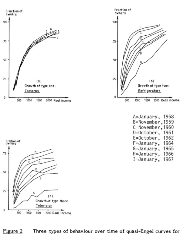
On the basis of cross-section data on household incomes and durable goods ownership for twelve different years, Bonus derived bundles of quasi-Engel curves, which turned out to fall into three distinct categories as illustrated in the tree graphs of figure 2.

Fraction of Fraction of owners owners 1 100 - 100. 4 d

.50 .50-.25 ' .25-4 (a) (b)

Growth of type one: Growth of type two:

Cameras Refrigerators

o . , . . v 0 . . . . 7

500 1000 1500 2000 Realincome 500 1000 1500 2000 Real income

A=January, 1958 B=November,1959 C=November,1960 D=October, 1961 , E=October, 1962

5611492 °f

F=January, 1964

G=January, 1965 H=January, 1966 I=January, 1967 .75 ' .50

.25 1 (C)

Growth of type three Television

560 1600 1st 2600 Reul ome

Figure 2 Three types of behaviour over time of quasi-Engel curves for

durable goods.

2.2.3.2

A quasi-Engel curve, obtained by averaging the ownership in different household income brackets for a particular durable (which is 0 or 1 for an individual household), is the discrete case equivalent to the classic Engel

curve. The change over time of the quasi-Engel curves found in

successive cross-sections was classified in this way:

Type 1 (including cameras and projectors): No change over time was

observed in the quasi-Engel curves. Diffusion had consequently no role to play in the growth in demand that had occurred in the post-was period. Type 2 (including automobiles, refrigerators, and vacuum cleaners): The quasi-Engel curves were rising more and more steeply with time, while the asymptot of each curve seemed to have stayed the same.

Type 3 (including television and washing machines): Both the slope and the final asymptot of each quasi-Engel curve were increasing with time.

Vertical and horizontal diffusion.

Bonus found reasons for distinguishing two kinds of diffusion vertical

and horizontal diffusion. Vertical diffusion occurs when people are

learning about the existence of a new product, and are thus becoming "potential" owners of the product concerned. This corresponds to a shift

over time in the asymptot of the quasi-Engel curve: in the beginning of

the learning process not even the very richest own the new product, simply because they have no, or only a vague idea of what it is all about. Horizontal diffusion occurs when people are well aware of its existence,

but their taste for the product concerned is growing. This takes the

Operational expression of a decrease in the "critical income"*. With

regard to the shape of the quasi-Engel curves this means that these curves

are rising more and more steeply as time passes. It can also be

characterized such that a previous luxury product,a product that was

consumed only by the rich, is becoming a necessity.

* The critical income of a particular household is the lowest income

that the household thinks it requires to afford the durable item in question.

2.2.3.3

Concerning automobiles it was thus concluded by Bonus that in West Germany the learning process (the vertical diffusion) was already over in

the beginning of the post-war period. On the other hand, tastes for

automobiles have been on the rise during the whole period. In low and medium income brackets car ownership has been steadily increasing. Television is an instructive contrast case of type 3. Both vertical and horizontal diffusion have taken place in the post-war period. This stands to reason: the television was a genuinly new product after the second world war, whereas the automobile was introduced already after the first world war.

The shape of the aggregate growth curve.

The question is now what the findings as to the different behaviour of the quasi-Engel curves imply for the shape of the aggretage growth curve in each particular case?

To answer this question it is necessary to know the income distribution in the economy in question. Bonus argues that the income distribution in

West Germany is approximately log-normal. On this assumption it is

possible to conclude that for durable goods of type 1, for which neither vertical nor horizontal diffusion occurs, and type 2, for which only horizontal diffusion takes place, the growth curve will be a logistic. For durable goods of type 3, on the other hand, for which not only horizontal diffusion, but also vertical diffusion takes place - a true learning process

is going on the resulting growth curve will, in general, be skewed.

These conclusions are contrary to the conventional wisdom, and are worth spelling out in the way Bonus himself does: "It has long been held in the literature that a logistic growth curve reflects epidemic innovation diffusion, and may be taken as empirical evidence for such diffusion. This is not true .... .. a logistic growth curve results when no diffusion whatsoever is present... When there is diffusion by learning, a skewed growth curve is much mOre likely." (Bonus 1972, pages 673-675).

In the light of this conclusion, it can be observed that the modification of the TRRL models of car ownership previously described, from a "simple

2.3 2.3.1

epidemic curve" to a skewed growth curve is an indirect indication of the importance of the role of vertical diffusion for the growth of car ownership in Britain*. The approach of the National Road Administration in Sweden, in which a logistic curve for the car ownership as a function of

time only is assumed (for each particular life-cycle category), does not

seem very apt in this light: diffusion is the only factor taken into account income is assumed to be unimportant and yet the chosen

functional form is one which typically occurs when no diffusion takes

place and only the income effect is operative.

Evidence of diffusion and income effects in Sweden in the 19705

Quasi-Engel curves for dif_f_erenilifefyclecategories 1974-1978.

The last-mentioned Swedish model makes still less sense in view of the fact that in the course of the preparation of a road traffic forecast for

1980 2000 by the Road Administration, the development of quasi-Engel

curves in the 19705 was investigated. (This work was mainly carried out by Ilja Kordi of Prognoskonsult AB)**. And the clear result of this

investiga-tion was that hardly any diffusion effect could be detected in the life-cycle categories under study, but instead that income played a role for

car ownership, at least in single-person households.

A rather limited period of time was studied cross sections were taken for the years 1974, 1976, 1977 and l978 but quite interesting results

were obtained nevertheless thanks to the stratification made by life-cycle

category.

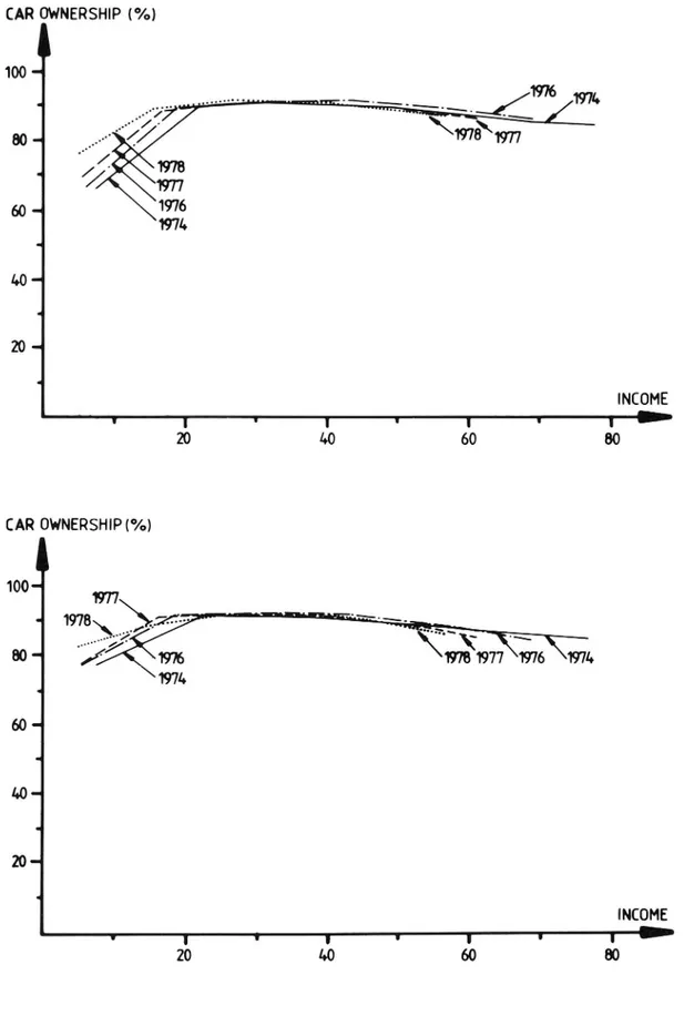
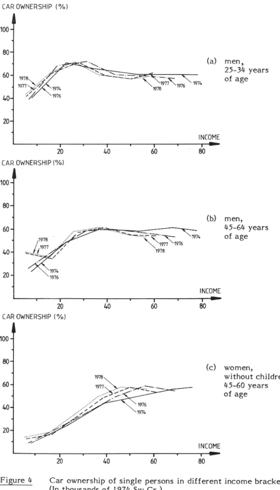
The diagrams of figures 3 and 4 give the results of the investigation. Along the horizontal axis household income is plotted, and along the vertical axis the percentage of households in each income bracket owning one or more cars is given.

* It should be noted that concerning car ownership in West Germany ,

Bonus concludes that "the observed growth curve was a logistic". Horizontal diffusion was going on, but no vertical diffusion remained in the post-war period. "It (the motor car) had been known for half a century when its tenfold spread began". (Bonus 1972, page 674).

** Statens V'agverk: Personbilstrafiken i Sverige 1980 2000.

Bilaga l: Ny prognos for personbilsantalet fram till ar 2000. P012 Bilaga 1. 1980-12-15.

CAR OWNERSHIP (°/o) 100-1

8°

\1978\19r77

INCOME .-I 80 8-4 5 8

CAR OWNERSHIP PA.)

I

10 d 0 m7\ /

INCOME

.-v f T ' y I ' '

Figure 3 Car ownership of married couples with children in different

income brackets. (In thousands of 1974 Sw.Cr).

Compared to the German experiences from the 19505 and 19605,

repre-sented by the curves of figure 2b on page , one feature of the Swedish

position in the 19705 is outstanding: for married couples the quasi-Engel curve seemed to have reached such a high level already in 1974 that the possible remaining horizontal diffusion taking place up to 1978 was confined to the very lowest income range, in which only some 5 % of the households are to be found. In 1978 the quasi-Engel curve seems to take the "extreme necessity" shape; it hits the ceiling almost at once, and

stays there throughout the whole span of incomes. In passing, let us say

that in relation to the situation in West Germany in 1968 just referred to, this is only to be expected: we would not be surprised if the corresponding quasi Engel curve looked the same in Germany in 1978 as in Sweden. So much for married couples. Car ownership in single person households is a rather different matter. So far as single men are concerned, it seems clear that no diffusion effect was operative in the studied time period. The ceiling, or asymptot of the quasi-Engel curves is, as seen, appreciably lower than for married couples*. This is an interesting fact, which is not commented on in «the study. Two possible reasons for this difference may

be that

(i) demand for travel is less for one person than for a family, and

(ii) single men frequently live in town centra close to work,

entertain-ment, etc. and/or where public transport is comparatively good.

For single women (figure 4c) it is possible to discern a small diffusion effect working between the years 1971; and 1978. Cross-sections from a number of earlier years are required in order to tell in which car

ownership diffusion stage the single women are. Are they still in the

stage of vertical diffusion, or is it only horizontal diffusion that is taking place? And in the latter case, is the diffusion period soon coming to an end, or are we still in the beginning?

* The falling tendency of the quasi-Engel curves should not be taken

seriously according to Kordi. It is explained by increasing disposal of company cars in the upper income ranges.

CAR OWNERSHIP (°/o)

100 #

80"

. "(a (a) men,

60 . A '\ .\ I 25-34 years 197a " m'Z LTJ-"F' 'm- of a e 1977\>?/ \EJ97'R1976\ 1971. 8 20" INCOME T l ' l V l ' V I "II" 20 40 60 80

CAR OWNERSHIP (°/oI 100- 80-(b) men, 60. 45-64 years J x 1971. of age 1977 1976

[ 0-

197a

20 1976 INCOME I I I l I I I l 4 20 40 60 80

CAR OWNERSHIP (°/oI

I

100- 80-(C) women, without children, 60- 45-60 years of age 40- 20-INCOME r - l I r ' I 20 1.0 6O 80

Figure 4 _{Car ownership of single persons in different income brackets.}

(In thousands of 1974 Sw.Cr.)

2.3.1.1 Two categories of special importance (1) first-car ownership of retired

2.3.2

people; (2) second-car ownership of married couples.

Two significant omissions in Kordi's presentation of quasi-Engel curves should be noted. The car ownership of retired pe0ple is one, and second-car ownership of married couples is the other. In Sweden roughly half of the still carless 1.25 million households consists of one or two retired It would be very interesting to see how the quasi-Engel curves The pr0portion of retired pe0p1e having a driver's licence is much lower than pe0p1e*.

have behaved in the post-war period for this life cycle category. for younger pe0ple, but is steadily increasing with time, and will, of course, become the same in due course, as the young pe0ple of today are getting old.

Another very interesting deve10pment that could usefully be examined by means of quasi-Engel curves from successive years in the 1960s and 19703

is second-car ownership. There are roughly 400.000 second-cars today.

The rate of growth in second-car ownership has been relatively high in recent years, but it is not known to what extent this can be explained by growth in real disposable incomes of households, or by other economic

factors, or whether it represents a separate diffusion process separate

from that of the first-car.

Income-elasticity estimation on cross section data

If one regards it as safe to conclude that practically no diffusion effect was working in the 19705 in Sweden, a cross-section estimate of the income-elasticity of car ownership would be quite useful both for insert-ing in a time-series analysis of the past deve10pment, and for forecastinsert-ing. In the course of the work on public tranSport problems in Stockholm by the so called LAKU-committee of inquiry, a car ownership forecasting model was developed by Staffan Algers, the parameters of which were

estimated by cross-section analysis**. By basing a forecasting model

exclusively on cross-section data, time itself as a representative of the

* Source: SCB, RVU 1978

** Staffan Algers: Prognosmodell f'or bilinnehav.

4. 1973.

VTI RAPPORT 251 A

diffusion effect is (implicitly) assumed to have no effect on the develop ment of car ownership. The question that we now will address is in the first place the historical one, whether it is true that no diffusion effect has been operative in the post-war period in Sweden.

Fortunately for our purpose, the LAKU-model has recently been used with a view to examining whether the values of the coefficients estimated in the beginning of the 19705 are stable, i.e. were the same both before and

after the year of the cross-section. Before the results of this examination

is presented, the model itself should be briefly described.

In 1972 observations were made in 136 neighbourhoods in the Stockholm

area, of the average car ownership of households, on the one hand, and of

average household income, household size, and the user cost of public transport relative to making different trips by car to/from these neigh

bourhoods, on the other. An index was calculated for the latter which

included the difference between the applicable public transport fare and the corresponding car running cost, car parking costs, the difference

between travel time by public transport and by car, the number of

changes, and the total waiting time incurred going by public transport. It was assumed that the log of the ratio of the number of carowning households to the number of carless households is a linear function of the aforementioned explanatory variables. The main result of the regression analysis can be summarized in this way:

if,

= 8,27 + 0,03 v + 0,58 H + 8,301

(1)

log

P : car ownership (i.e. proportion of households, with at least one car,

or "probility of car ownership", if you like).

Y = average household income before tax H = average household size

I : index of the relative cost of public transport versus private car for

non-work trips

It was pointed out that this result implies an income-elasticity of car ownership of about 0.5.

2.3.2.1 Problems of testing cross-section estimates on time-series data

To test the stability of the coefficients over time, the real values of the explanatory variables for each year of the period 1955 1979 were inserted in the model*. In figure 5 it is shown how the actual development of car ownership in this period compares to that obtained by the model. In the year for which the model was calibrated - 1972 - the two curves, of course, intersect. Going backwards from 1972, the two curves are very close as seen. After the second point of intersection in 1963, however, a

widening gap appears. In 1955, the first year of the comparison, the

model estimate is some 70 96 above the actual figure.

It is close to hand to think that the initial discrepancy is due to a diffusion effect, still lingering on in the mid-fifties, but gradually running out to be completely finished by 1963. A supplementary explanation is offered by Staffan Widlert. He points out that the real price of cars, which is not included in the model, stayed roughly the same in the 1963-1972 period, whereas it was falling appreciably in the second half of the 19505.

For the time period 1972-1979 three curves are given in figure 5. The upper curve represents the actual develOpment of car ownership, the middle curve has been obtained in the same way as was just described concerning the period before 1972, and the lower curve represents a forecast made in 1973 (by LAKU). At that time the true values of income etc. for the rest of the 19705 were not known: the LAKU-forecast assumed a rate of growth in income of 2.5 96 per annum. This turned out to be very nearly true as an average, but substantial deviations from this average were recorded for individual years.

Does Algers/Widlerts' combined cross-section and time-series analysis represent the last word as regards the existence of a diffusion effect? One reservation has to be issued on account of the confinement to the Stockholm area. Another question may be, whether the conclusion that the diffusion process seems to have come to an end already in the beginning of the 19605 is equally true for all life-cycle categories? If the material were stratified by life-cycle category in the way it is done in the forecasting model of the National Road Administration, would the same pattern come out for each category?

* See Staffan Widlert: Biltathet i Stockholms Lan.

Trafikkontoret, Stockholms Lans Landsting 1981.

CARS/1000 PERSONS // Forecast 2so~ 200 $0~ 100 50« 11111r1 11v1111r11111YYT I" Ar 19LS so 55 60 65 7o 75 80 YEAR

faktisk utveckiing (actuai deveiopment)

-- -- modeiiberaknad utveckiing (estimated deveiopment)

o startar fbr modeiiberakning (base year for mode1 estimate)

Figure 5 Actua], estimated, and forecasted deveiopment of car ownership (cars/1000 peopie) in Stockhoim region.

A methodological question-mark has also to be mentioned. The income-elasticity of demand obtained by cross-section analysis is comparable to the long-run income-elasticity as seen over time: that is, to take an example, if the disposable income of households is increased by, say 5 %

in year t and stays at the new level until year t + 10, and all other things remain equal, too, an increase of lO 0/0 in car ownership observed in year

t + 10 compared to year t would indicate a value of the long-run income-elasticity = 2, while the effect registered in the first year (t, or t + 1)

corresponds to the short run income-elasticity. On theoretical grounds

one should expect these two elasticities to be different, at least so far as durable goods are concerned. Evidence from studies of consumer durables in general show also that the long-run elasticity and short-run elasticity

differ substantially*. Bearing this in mind, the real test of whether the

cross-section elasticities of car ownership with respect to income and household size have sufficient predictive power, is to what extent the long-term trend in car ownership, rather than the actual development in the years close to the year of the cross-section, can be explained. By this criterion, the outcome of Widlert's test of Algers' model gives rise to more mixed feelings: looking forward from 1972 the model hits the mark, while looking backwards it is well off the mark.

* See e.g. Houthakker H.S, 6c Taylor L.D.: "Consumer demand in the

United States 1929-1970. Cambridge, Mass., 1966 VTI RAPPORT 251A

2.4

2.4.1

Long term forecasting: the issue of the saturation level

Having estimated the coefficient of a demand model on time series and/or cross-section data, the standard procedure is, when it comes to forecasting, to make predictions of the values of the explanatory vari-ables for the future date concerned, and insert these values in the model. The basic condition for the relevance of this procedure is that one believes in one's model; that is to say, one has reason to believe that the estimated coefficients are stable also in the future. In a case like the present one, the two general forecasting problems of

(a) changeability of tastes,

(b) the existence of a saturation level

are particularly notable. Both a change in taste for motor cars, and the approaching of the saturation level of car ownership will express them-selves in changes of the coefficients of the demand function. We have been discussing the importance for the demand for cars of growing tastes

for cars under names such as "the demonstration effect", "the learning"

or "diffusion process" and it would be rather unimaginative to think that

today's tastes would stay constant for a very long time. The idea of a saturation level of car ownership has been prominent in "'future of the automobile" discussions for several decades. Now the deveIOpment on the continent of the automobile (North America) has advanced so far that

something more firm can be said about the long-standing issue of the

saturation level. Before that it is appropriate to take up a problem of definition: for a long time the discussion has been rather confused because the concept of a "stationary equilibrium" and the concept of the "satura-tion level" of car ownership have frequently been mixed up.

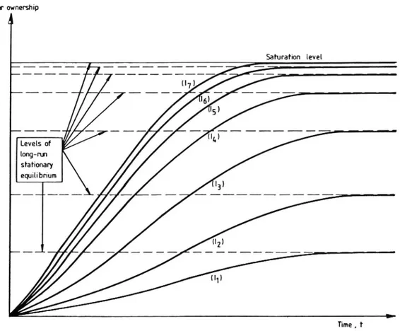
Stationary equilibrium of car ownership vs. the saturation level

By means of two diagrams (fig. 6 and 7) the difference between these two

concepts will be clarified, and the proper definition of the saturation level of car ownership will, hOpefully, come out as self-evident. First, take the

hypothetical case of real income (as well as the distribution of income)

remaining constant over time.

Car ownership

ll

Saturation level _ _ _ _ _ -- _ _ - _

Levels of long I m stationary equilibrium

Time,t

Figure 6 Given the income per head (I) the car ownership will sooner or

later, after a period of diffusion, reach a stationary equilibrium. Following the introduction of the motor car the total stock of cars will be growing up to a point where the demonstration and learning effects are no longer working. This represents a stationary equilibrium of car ownership. ("Stationary" implies that the economy is not growing, and, therefore, as long as tastes are given, the same quantities of goods and services are

produced and consumed each successiv periodof time.) The higher the

given level of income, 11, 12, I3 ...., is assumed to be, the larger the total

stock of cars will be in stationary equilibrium.

However, there is presumably a finite, highest level of car ownership

"the saturation level" which would not be exceeded whateverthe level of

income will be. In other words: a saturation level exists if the

hypotheti-cal growth curves - each associated with a given income are converging

for higher and higher incomes. The final saturation level is obtained when

the growth curves for successively higherincomes no longer shift but

coincide. Needless to say, this hypothetical reasoning only provides a definition of the saturation level; it is no proof of the existence of such a

level.

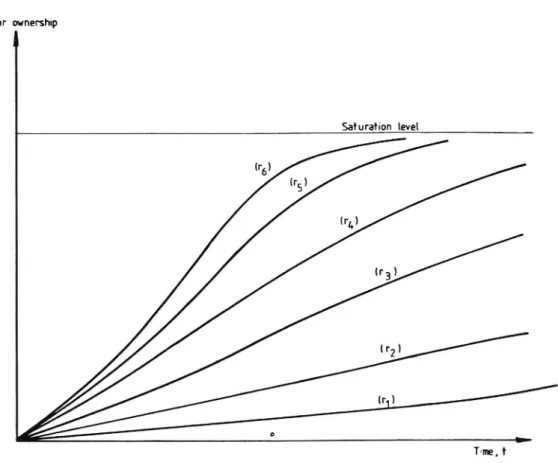
In the past motor car diffusion and economic growth have occurred at the same time. The car ownership growth curves that have been observed in different countries are of the kind illustrated in figure 7 below. In this diagram each curve presumes a certain average rate of economic growth. The basic hypothesis is simply that the car ownership growth curve sets out at a steeper and steeper climb, the higher the rate of economic

growth (r1, r2, r3, ...) will be. Eventually, however, all curves will meet at

the saturation level -- provided that a saturation level really exists.

Car ownersz

ll

Saturation level (r6) (r ) (FL) 3 (r2) (r) TImeJ

Figure 7 Car ownership growth for different rates of economic growth. Hypothetical example.

The main difference between the diagrams of figure 6 and figure 7 should

be noted. The stationary equilibrium levels of figure 6 depend on the

income level assumed in each case. If the level of income is not very high, the car ownership will never reach the saturation level. In figure 7, on the other hand, where some economic growth is assumed in every case, all curves will eventually come together at the saturation level. In passing it can be noted that in the hypothetical cases of figure 6, the diffusion period is clearly identifiable: it starts at time 0, and ends when the stationary equilibrium is attained. In the realistic cases of figure 7 the duration of the diffusion period is in no case possible to discern from the car ownership growth curve. It may end at an early or rather late stage in the development towards saturation there is no a priori argument in

favour of one or the other alternative. However, it would be an

extremely unlikely coincidence, were the diffusion period to last right up to the time when the saturation level has been obtained. As has been pointed out in the previous discussion, it is of central importance for making forecasts to know whether or not the diffusion period is over. Were it wholly a passed stage, car ownership would not continue to grow in a stagnant economy, and would most likely fall, if car prices and the cost of fuel would go up in real terms. On the other hand, if the diffusion were still going on, car ownership may well continue to grow even in a stagnant economy.

To summarize, we propose the following definitions of two key concepts: Stationary equilibrium of car ownership 2 Level of car ownership even tually obtained in a hypothetical case of income and relative prices remaining constant for ever.

Saturation level of car ownership : Level of car ownership which will not be exceeded, neither with further rising income and/or falling relative price of car travel, nor with time (Note that this definition does not tell if a saturation level exist, or, if so, when and where it will be reached).

2.4.2

An additional reservation should be issued: the saturation level thus defined assumes that, after the diffusion period is completed, tastes remain constant from then on. This is by nomeans a logical necessity. For example a superior mode of transport may appear some time in the future, which will make the motor car obsolete, or if "communication" becomes a strong substitue for "transportation" as is foreseen in some visions of the post-industrial information society, the saturation level of car ownership, as defined on the basis of the present order of preferences, may never be attained even if everyone would be so well-off that a car could easily be afforded by every person 18 years of age or older.

US evidence of the saturation level of car ownership

Having defined the concept of the saturation level, the question is now:

where is the saturation level of car ownership? Note again that this is

not necessarily the ultimate level, i.e. the level of car ownership that will eventually be attained some time in the future. In a stagnant economy, for example, the ultimate level of car ownership is not equal to the saturation level. In a stagnant economy the relevant question is, when it comes to forecasting, what the stationary equilibrium level will be. The following discussion of what the saturation level may be must not be taken as a long-term forecast.

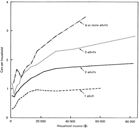
Let us see what the situation is in the U.S.A. today. The following two graphs are quite revealing. In figure 8 cars per hosehold is plotted against household income for household consisting of l, 2, 3, and 4 adults,

respectively. As seen, all curves seem to have asymptots at levels

corresponding roughly to the applicable number of adults. This pattern is even more apparent when the same information is given in the form of the

graph of figure 9. There cars per adult is plotted against household

income per adult. It is striking how close the four curves are. It seems that household size (number of adults) is practically inconsequential for car ownership as measured per adult. Also a saturation level of nearly one car per adult is very suggestive.

4 0/ / ./ \ 4 or more adults 3 - .l I/

./

...-'0 _{...u \}... ° g "" " 3 adults a / .c 2 -g /'/ 0'. 4 U ' 2 adults 1 ,. . _ _ _ _ _ _ _ - - '-2. I o - " \ I 1 adult I I I I I 0 L L L 1 0 20 000 40 000 60 000 80 000 Household income ($)

figugg_§ Cars per household and income per household, US NPTS, 1977-78 1.0 0.8 Ca rs pe r ad ul t .0 cn .o a 0.2 -0 _{o 10 000}' _{20 000}L I 30 000

Income per adult ($)

Figure 9 Cars per adult and income per adult, US NPTS, 1977 78

2.4.3

Is this saturation level also applicable to other countries than the U.S.A.? In other words: if the minimum income per adult in countries like England or Sweden would eventually reach such a high level as, say $ 25.000 per annum, would this result in the car ownership getting close to one car per adult?

British conditions, argues that because of the "greater tendency in Britain Tanner, in commenting on the relevance of the US figures for

to live in cities at relatively high densities compared with the US the

saturation level of around one per adult should be scaled down, possibly by about 25 per cent" (Tanner, 1981 page 4). For Sweden this reservation is

less valid. On the other hand, if we in Sweden would ever become that

well-off, it is likely that we could afford substantial improvements in

public transport quality, which might have a moderating effect on the

saturation level of car ownership.

The main uncertainty, however, remains concerning economic growth. Will incomes ever grow to such levels, and if a certain amount of deveIOpment optimism were justified, how long will it take before such

levels of income have been obtained?

Cars per adult vs. cars per household

An interesting by-product coming out from the study of the US saturation level of car ownership is that cars per adult set against income per adult seems to be a more relevant relationship than the more common one of

cars per household set against income per household. Tanner (1981) draws

the conclusion that the US data indicate that car ownership should be regarded more as a personal attribute than a household attribute. It is interesting to note that the available Swedish data suggest the same

thing. This can be checked preliminary by looking at the quasi-Engel

curves on pages 21 and 23. In 1978 some 90 per cent of married couples in the household income range exceeding 20.000 Sw.Cr. had at least one car. Add to this the frequency of a second-car, which is about 30 96 in the

upper income range. That gives a level of car ownership per adult of

about 60 96 for an income of l+0.000 Sw.Cr. per adult. Now look at the graphs of page 23, giving quasi-Engel curves for single-person households. At an income of 40.000 Sw.Cr. it is seen that more than every second single woman had a car in 1978, say 55 %, and about 65 96 of the single

men (taking an average of the two age groups given). That is to say, car

ownership per adult of single-person household was the same as that of married couples, i.e. about 60 %, which, by the way, is not far from what

applied in the US at the same time.

3.1 TO TA L SA LE S x IO 'Z I w J __ ;7 -=

MODELS WITH A VIEW TO EXPLAINING FLUCTUATIONS IN CAR PURCHASES

The change of focus from car stock to car investment flow

The basic characteristic of the car ownership growth curve estimations

previously described is that the long-term M in car ownership is the

object of study. Cyclical variations around the trend, or other short-term fluctuations coming into view when looking closer at the actual path of deveIOpment, are of secondary importance when the ultimate purpose of the models is to make long-term forecasts of the future level of car ownership. Suppose instead that we want to study the derivative of the growth curve, i.e. the derivative of the car stock with respect to time, or, alternatively, total car purchases in consecutive periods of time, how does the statistical picture look in this instance?

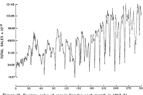
The pattern of car sales over time exhibits in fact wide fluctuations. The

figure below shows the monthly sales of cars in Sweden during 19#7-7l.

As seen, the figure of the highest month is seven times greater than that

of the lowest month.

[2 I .43 IO3.95

\l U l

69.00

. .;

53.52 i *l g 34.05 l6.57 L l l l l 1 1 l l l l l O 30 60 90 I20 l50 ISO 210 240 270 300 I I 5 2 ? " , : 3 . _ "2 . 2 5 : 3 3 "

r

. _ . _ _ . . _ _ _ . . . . 4 -_

Figure ID Factory sales of cars in Sweden each month in l9lL7-7l

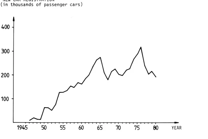
Annual sales, as expected, show less variations, but some substantial fluctuations have been observed in recent years, although the increasing trend is, perhaps more striking so far as the first two post-war decades

are concerned.

NEW CAR REGISTRATION

(in thousands of passenger cars)

ll

1.00

-300 *

200 *

100

Figure 11 Annual new car registrations in Sweden 1946 1980.

purchases, as distinct from the development of the trend in car owner-ship?

From the point of view of macro-economic stabilization policy, the short

term fluctuations in consumer durable investments constitute a major

problem comparable to the more notorious problem of the irregular

pattern of investments by firm. In neither case wholly satisfactory

models of short term forecasting have been developed. To the producers of consumer durables including automobiles it also makes an appreciable difference, whether the expected total sale for the next two-year period

will be A and A, 1.5 A and 0.5 A, or 0.5 A and 1.5 A. Anyway a lot of

effort has been put into the modelling of short term fluctuations in car purchases with the basic purpose of making short term forecasts of car

purchases, either as part of an economy-wide macro model, or exclusively addressed to the car industry. In the former case the car demand model is typically a sub model of a model for total expenditure on consumer

durables.

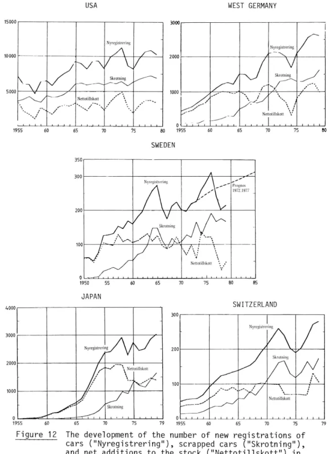
When annual car investment is under study rather than the development of car ownership, the first fact to bear in mind is that a large part of total car investment is to be characterized as replacements. In Sweden like in

most other developed countries the number of cars scrapped per year is

nowadays of the same order of magnitude, or greater than the net

addition to the stock of cars. (See figure 12.) To predict total car sales it is

consequently as important to understand the causes of the need for car replacement as to understand the causes of car net investment. And these causes may well be rather different.

In the following survey of models for explaining car purchases we

distinguish in the first place between static and dynamic models. A static demand model is a "timeless" model in the sense that demand in each period is assumed to be independent of what has happened in previous

periods. This is the standard assumption so far as demand for non-durable

goods are concerned. For example, the demand for potatoes in year t is

independent of the quantity demanded in year t-l or any other previous

periods. At least for some durable goods this assumption does not seem

very fitting. If a certain person bought a car last year, he is unlikely to buy another this year. Dynamic models of demand have generally been considered necessary in cases of durable goods lasting for many years; that is to say purchases of durables in year t cannot be explained in a static context, cut off from events in previous periods.

39

USA WEST GERMANY

15000 3000 Nyregistrering 5 N . _ A yreglstrermg 10000 ~ ~ ///\ 2000 f \ \ 4/ Skrotning /\ 5 Skmmmg / ~ V Ava/\f I , _ -. 5000 <_\\v // _{r/ .u}. 1000 / ~"" s 'I ;:~u I1 / a N\ / Nettotillskolt , x a / x\ /y \s . l' I I «~ ,A .\ /"- x {I . '1. / _{3 r} '._{~\ [I}" x_3/ 5 1 - ," A n I 1 ,/ __/ Nettotillskolt 1' \ / / P11111111111111111111 O'IILI 1111 1111 1111111L 1955 60 65 7O '75 80 1955 60 65 70 75 80 SWEDEN 350 300 ( 1 Nyrcgislrcring 1 Prognos 1972,1977 A 200 / V Skrolning / K t .'\ 1mw\J/_ /// Ap; -Neltolillskoll _ E. 1 1 L 1 1 1 1 1 1 1 1 1 1 1 1 1 1 4 1 1 1 l 1 1 1 1 1 1 1 L 1950 55 60 65 70 75 80 85 JAPAN

4000

1

SWITZERLAND

300 I Nyregistrering 3000 A b A NyregislreriWJ s 200 / \/ A Skrotning 2000 I. ' _ a V \ Neltoullskolt .K » ~ / .I9'-x / -' 100 , -_ ,'\ _ r,4 x f I If u / L-Hb ~h d f. ,T/ Nettolillskott ./ __ ,_,_._./ /__/\/ " .. / Skrotning L1 0 .1 - M « 1 1 1 1 1 I 1 1 1 1 L 0 1 1 1 J 1 1 14 1__1 1 L1_.._L.1L.._J.J_, 1955 60 65 70 75 79 1955 60 65 70 75 79

Figure 12 The deveiopment of the number of new registrations of

cars ("Nyregistrering"), scrapped cars ("Skrotning"), and net additions to the stock ("Nettoti1iskott") in

the postwar period.

Source:

Lars-Jacobsson:

Personbiismarknaden under 1980-ta1et. Handeisbankens smaskriftserie 18.

3.2

In Sweden a static model has been developed by Lars Jacobsson. His work

(Jacobsson, 1972) can to some extent be regarded as following up a

tradition of econometric studies of the car market carried on at the

Research Institute of Swedish Industry (IUI) including (Bentzel 1957), (Wallander 1958) and (Endredi 1967) but the approach chosen by Jacobsson

is wholly his own.

A static model

Jacobsson has developed two separate models for explaining car net investment, and car scrapping, respectively (on the implicit assumption that car scrapping equals car replacement investments).

When it came to explaining the net addition to the car stock in the years

1958-1971 two significant determinants were found a proxy for the

change in real income (or standard of living), and the change of an index

of used car prices*. The result of the regression analysis can be summar

ized by this equation:

A Kt = 83795 + 6264 c 15601;

(1)

(R2 = 0.89)

A Kt : Net addition to the stock of cars in year t

d 2 percentage change in total private consumption

P. : percentage change in used-car price index

As can be seen in figure 14, the model estimate is in good agreement with the actual figures for the net additions.

* It was rightly argued that a first time owner usually buys a used car.

However, the connection between the demand for used cars and the demand for new cars was not explicitly accounted for.

Thousands 130 F 120 ~ 110 100 *-90~ so - _. estunated actual 70/: OT 1 l 1 1 1 1 l 1958 60 62 64 66 68 70

Figure 13 Actual and estimated net additions to the car stock in 1958-71.

Two points are worth making.

(1) As is seen, the values of the net additions fluctuate around the 100,000

cars level. The constant of equation (1), taking a value of 83,795,

consequently "explains" a lot of car net investments. That is to say, if

income (or total private consumption) as well as prices of used cars would

stay constant, more than 80,000 new carowners would all the same be

registered each year according to equation (1). The cutting short of the

vertical axis of figure 13 serves to somewhat disguise the fact that the passage of time is by far the most significant factor explaining car net

investments.

(2) The previous point does not mean that the income-elasticity of car

demand indicated by equation (1) is very low. On the contrary, it seems to

be rather high. It is just that the percentage change in income has been relatively modest in the period under study. The value of the coefficient of C indicates that an one-percent increase in household real income