Developing a soprano classifier using FIR-ELM neural network

School of Innovation Design and Engineering

V¨aster˚

as, Sweden

Thesis for the Degree of Master of Science in Engineering - Robotics

30.0 credits

DEVELOPING A SOPRANO

CLASSIFIER USING FIR-ELM

NEURAL NETWORK

Peter Cederblad

pcd11001@student.mdh.se

Examiner: Mikael Ekstr¨

om

M¨alardalen University, V¨aster˚

as, Sweden

Supervisor: Branko Miloradovic

M¨alardalen University, V¨aster˚

as, Sweden

Abstract

This thesis aims at investigate the feasibility of classifying the soprano singing voice type using a single layer neural network trained with the FIR-ELM algorithm after that the monaural auditory mixture has been segmented with the Harmonic, Percussive and Residual, HPR, decomposition algorithm, previously introduced by Driedger et al. Two di↵erent decomposition structures has been evaluated both based on the same HPR decomposition technique. Firstly one single layer that only take advantage of the result of the more pure harmonic and the more pure percussive components of the signal. Secondly, one multilayer structure that further decompose both the harmonic and the percussive components but also takes into account the components that can not be clearly categorized as neither harmonic or percussive components, these are the residual components. The result of the classification was up to 98.5 % after using these segmentation techniques, this shows that it is feasibly to classify the singing voice type soprano in an monaural source recorded in a non-professional environment using the FIR-ELM algorithm.

Table of Contents

3 Motivation 4 4 Method 4 5 Theory and Design 5 5.1 Voice production . . . 5

5.2 Human auditory system . . . 5

5.2.1 Harmonic-Percussive-Residual decomposition, HPR . . . 6

5.2.2 Melody-Residual decomposition, MR . . . 8

5.2.3 Transient-Residual Decomposition, TR . . . 9

5.2.4 Sparse-Low rank decomposition, SL . . . 9

5.2.5 Mel Frequency Cepstrum Coefficients, MFCC . . . 10

5.2.6 Single layer Feedforward neural network . . . 16

5.2.7 Bidirectional Recurrent Long Short-Term Memory neural network, BLSTM NN . . . 17

5.2.8 ELM neural network . . . 17

5.2.9 Regularized ELM neural network . . . 18

5.2.10 FIR-ELM-neural network . . . 18

5.3 Design . . . 20

5.4 Audio samples . . . 21

6 Results and Discussions 23 6.1 Experiment setup . . . 23

6.2 Result for research question 1 . . . 23

6.3 Result for research question 2 . . . 23

6.4 Result for the hypothesis . . . 23

7 Conclusion 25

8 Outcome 25

9 Future work 26

1

Introduction

Segmenting music accompaniment from singing voices is important in many applications in the music industry, e.g. it can be lyric- and emotion recognition or music alignment.

The human auditory system has a very high capability of separating music and voices in the acoustic mixture. This extraordinary capability has not yet been truly implemented in machine learning. However there are several algorithms that has shown good success in di↵erent areas. In this thesis several of these algorithms will be used in order to decompose opera music from the singing voices from a monaural source. This thesis aim at investigate the feasibility of using the FIR-ELM training algorithm for a single layer neural network in order to classify the singing voice type Soprano from other voice types in a monaural source.

Previously work done by Pawel et al. in [35] shows that singing voice types can be classified with good accuracy. Pawel et al. used an single layer neural network, and trained it with an ordinary backpropagation training method. The result for the soprano singing voice type classification was 94.1%. However, in Pawels work their are six classification outputs(bass, baritone, tenor, alto, mezzo-soprano and soprano) but only vowel sounds are used.

1.1

Problem formulation

In automatic singing voice type classification some research has been performed in recent years e.q. [35] using ordinary feedforward artificial neural networks. However these researches involves singing samples recorded in a cappella (no accompaniment) and another limitation is that the samples often only constitute vowel sounds. These previous researches shows that it is feasibly to classify di↵erent singing voice types with good accuracy using neural networks. Little or no research has been conducted in classical singing voice types first separated from ordinary opera music in monaural recordings. This makes it interesting to investigate the possibility to train and evaluate the result from a new training algorithm for single layered feedforward neural networks with inbuilt linear filter called the Finite Impulse Response Extreme Learning Machine neural network, FIR-ELM neural network that previously has been evaluated in classifying Chinese folk songs in [5].

1.2

Hypothesis

It is possibly to classify the singing voice type, soprano in the opera performance Medea using a FIR-ELM neural network.

1.3

Research questions

1. Is it feasibly to classify opera vocalists singing voice type using FIR-ELM network?

2. Will the subjective accuracy of the audio decomposition increase with a second separation factor in the HPR decomposition algorithm?

2

Background

This master thesis is part of a collaborative project that aims at investigating how robotics can contribute to the art of opera. In order to sharpen this projects goal a specific case has been chosen: A marionette robot shall be developed that reflects the role played by Maria Callas as Medea, which is based on the ancient Greek tragedy with the same name.

One aspect of this work is the collaboration with two researchers that are active in scenography and opera, ˚Asa Unander-Scharin and Carl Unander-Scharin, respectively together with students at M¨alardalens University. The project has been divided into two groups. The physical robot will be designed and developed under the supervision of the Unander-Scharin couple. While the author of this thesis work will develop a singing voice type classification system that lets the vocalists control the robot in an intuitive way.

The main goal of this thesis work is to develop a voice type classification system, in order to let the vocalist interact in an intuitive way with the robot during a live performance.

2.1

State of the art

There are two major path considering singing voice separation techniques. Decompose the input signal in one step, and base the voice extraction on one voice feature, or decompose in multiple steps and use di↵erent algorithms in each step inorder to extract di↵erent characteristics from the voices. One major characteristic that easily can be detected in the human singing voice is the harmonic structure, unlike from the accompaniment that has a large amount of percussive structure in the mixture. This is utilized by several researchers [1,8,9]. Other highly strong characteristics is the contrast between the repetitive rhythm in the accompaniment and the variance in the singing voice, this is exploited for example by Leglaive et al. in [4]. A third alternative is to consider the spectral sparseness, which is being used by Po-sen et al. in [2].

Driedger and Muller showed in [1] that by decompose the audio signal in three layers, they could separate the vocalist sound from the accompaniment with good result. However, their study uses di↵erent amount of energy in the singing voice part of the music from the accompaniment part. When the energy levels are equal, their classification results deteriorate.

The ELM training algorithm was first developed in 2004 by Huang et al. in [16], since then the algorithm has evolved in several branches. It has been shown to work well in several di↵erent applications such as automatic speech recognition systems, computer vision, navigation systems and classification problems just to mention a few [18]. 2014 Khoo and Sui Sin investigated the possibility to enhance the ELM algorithm with an finite impulse response, FIR, approach for the initialization of the input neurons weights. Their research was focused on classifying Chinese folk songs, focusing on separating the folk songs from the Han district from other districts.

3

Motivation

In the recent decades interest in automatic singing recognition has started to progress. However, very little work has been done in the field of segmenting opera music from the vocalists and classifying the di↵erent voice types. Most of the algorithms that have been developed through the years have been tested on popular music and country songs.

4

Method

The method during this thesis work was to search for information on how opera music, the human singing and auditory mechanism works and in parallel investigate state of the art in vocal-music separation. When an previously tested approach was found that had good result on popular and country music, and it had not yet been tested on opera music, it was decided to follow this approach and investigate the possibility on segmenting opera vocalists and accompaniment using this algorithm. The algorithm was implemented in MatLab and all the tests and evaluation was made in this environment.

Since the author of this thesis could not find a suitably dataset for training and testing the network, three datasets hade to be recorded. One for training, one for testing the neural network and one in order to evaluate the network against the Medea play.

5

Theory and Design

This section will first briefly introduce the human vocal apparatus and the human auditory system. After this, theory about the di↵erent algorithms and the overall system design will be explained.

5.1

Voice production

The voice production can be divided into two main blocks: The audio source and the modulations. The audio source for humans is the speech apparatus, which can be further divided into three sections. Three main systems:

1. The respiratory system, which contains the lungs, thorax, thoracic diaphragm and the tra-chea. The purpose of the respiratory system from an vocal point of view is to provide the glottis and the vocal tract with an airstream. The respiratory system can be seen as a compressor.

2. Phonation system includes the larynx and the vocal folds. Phonation means generating sound by means of the vibrations of the vocal folds. It is this sound that is the voice source and can be defined as the primary sound. The vocal folds can be seen as an oscillator

3. Articulation system is the vocal tract and it includes the areas above the larynx, throat, oral cavity and nasal cavity. Also the tongue and lips that are a few of the surrounding structures of the cavities. In the vocal tract the primary sound is further modified by the influence of the di↵erent articulators, e.q. the tough shape and placement in the mouth. The Vocal tract can be seen as an resonator.

Overall the voice organ has very much similarities with an wind tunnel. The lungs provide an airstream that flows in to the tunnel(The vocal tract) through the vocal folds. The oscillations of the vocal folds changes the pressure distribution inside the vocal tract and resonance frequencies takes place at di↵erent locations in the vocal tract. These resonance frequencies are the formants, which are the pronounced sound that humans use to communicate with each other, both in speech and in singing. In singing this means that the vibration rate of the vocal folds is equal to the tone that for instance a soprano is singing. If a Soprano uses the note A5 which has the frequency of 880 Hz, her vocal folds vibrate with a rate of 880 Hz.

The formant frequency is dependent first of all on the length of the vocal tract. In males this is an average on 17.5 cm which gives a first formant frequency on 500 Hz(1/4 length). The second formant is 3/4 length and so on, see Fig1. The di↵erent formants depends on di↵erent articulators in the vocal tract. These articulators are what constitutes the modulation in the voice production. Also the reason that a singer can easily be heard in an opera over the orchestra is due to the singer formant... However the soprano song type seems to be missing this extra formant. The singer formant comprises of 3, 4 and 5th formant. The energy of the combination of these three is similar to the energy in the first formant.

5.2

Human auditory system

The human auditory system is conducted by two main parts. The sensory organ (the ear) and the sensory system. The physical structure can be divided into three parts; The outer ear, the middle ear and the inner ear. All three parts play there role in the auditory perception. The physical form of the outer ear (the auricle) makes the sound waves mitigate and/or bounce around before entering the ear channel. Some frequencies slips right in the ear channel. The auricle acts as a first filter in the auditory system. Sound waves that has a frequency that we humans can not hear are reflected. The structure also acts di↵erent on low frequencies from high frequencies. Low frequen-cies are more or less directed in to the ear channel, while high frequenfrequen-cies can bounce around and

Figure 1: Shows the positions of the four first formants in the vocal tract [24].

then create an delay. This small delay can cancel out new incoming sound waves that is twice the delay time, the delay also interact with neighboring frequencies. This creates a complex pattern. The ear channel will then amplify the incoming audio signal if it is between 3 and 12 kHz. When the sound wave reaches the end of the ear channel it hits the eardrum (tympanic membrane) [25]. The sound pressure will be amplified up to 20 times by the ossicles in the air-filled cavity that con-stitutes the middle ear. After reaching the end of the ossicles structure, the vibrations transmits into fluid energy in the cochlea via the oval window and the two ducts, tympanic and vestibular duct that is filled with a fluid called perilymph. This fluid has a di↵erent potential then the en-dolymph that fills the cochlear duct. It is in this duct that the organ of Corti is located, and sound waves are transformed into electrical signals for the brain to interpret with the help of the hair cells and the basilar membrane [25].

5.2.1 Harmonic-Percussive-Residual decomposition, HPR

The first block in this algorithm decomposes the input audio signal into three main blocks following the procedure of first transforming the input audio signal into its spectrogram. Second, this spectrogram will be exposed to a median filter, first in the horizontal direction and then in the vertical direction. It is shown in [7] that percussive sound has a vertical structure while harmonic sound has a horizontal structure [8]. However, these two output blocks usually contain some non-harmonic components in the non-harmonic block and non-percussive components in the percussive block. In order to reduce these misplaced components a third block will be used as has been done by Driedger et al in [8].

The separation of harmonic components and percussive components are done as follows: Divide the signal into T frames, and then compute the short-time Fourier transform (STFT) over all the frames. Now the spectrogram X has been created. Expose the Magnitude spectrogram Y = abs (X) with a median filter first along the time axis and then along the frequency axis. Two enhanced magnitude spectrograms are created.

˜

Yh:= median(Y (t lh, k), , Y (t + lh, k)) (1)

˜

Yp:= median(Y (t lp, k), , Y (t + lp, k)) (2)

The above procedure yields the two main outputs, the harmonic block and the percussive block. The Extended Harmonic-Percussive separation of audio signals [8] enhances the purity of these blocks by using a separation factor, . By creating two mask matrices, one for the harmonic components and one for the percussive components the third residual block can be constructed. Set = 1. The below operators> and >= are binary hence the output will be 0 or 1.

Mh(t, k) := ( ˜ Yh(t, k) ˜ Yp(t, k) ) > (3) Mp(t, k) := ( ˜ Yp(t, k) ˜ Yh(t, k) ) >= (4)

By multiplying the Mh and the Mp masks with the spectrogram X, we get the components

constituting the two blocks. According to the following equation.

Xh:= X(t, k)⇤ Mh(t, k) (5)

Xp:= X(t, k)⇤ Mp(t, k) (6)

However, by adding the constraint > 1 equation 3and4 will take the form of: Mh(t, k) := ( ˜ Yh(t, k) ˜ Yp(t, k) ) > (7) Mp(t, k) := ( ˜ Yp(t, k) ˜ Yh(t, k) ) > (8)

Now there will be some parts of the signal that does not fit in any of the two main blocks. These components will constitute the residual block, and are calculate as:

Mr(t, k) := 1 (Mh(t, k) + Mp(t, k)) (9)

Xr:= X(t, k)⇤ Mr(t, k) (10)

The higher value of , the cleaner the two main blocks will be, this will also increase the amount of components in the residual block. In this thesis work one extra separation factor is added, in order to be able to adjust di↵erent amount of components from the harmonic block and the percussive block into the residual block. Therefore h and p are used instead in7and8, this yields the two

equations that this thesis uses:

Mh(t, k) := ( ˜ Yh(t, k) ˜ Yp(t, k) ) > h (11) Mp(t, k) := ( ˜ Yp(t, k) ˜ Yh(t, k) ) > p (12)

After that the signal has gone through equation5and6the result transfers back to time domain by using an inverse to the STFT.

Now there will be an second run through the sum of the harmonic block and the percussive block in order to enhance the three blocks.

xhp:= xh+ hp (13)

Because the harmonic components and the percussive components are strongly coupled [8]. the following mixture of components shall be the output blocks for the next phase.

xh:= xf irstrunh (14)

xp:= xsecondrunp (15)

5.2.2 Melody-Residual decomposition, MR

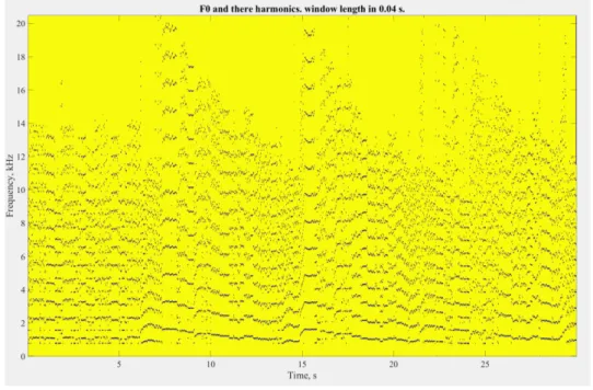
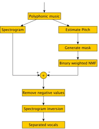
The Melody-Residual block consists of the most harmonic components in the audio signal both accompaniments and voices. The input for this block is the result from equation 14. The de-composition of the MR block follow the procedure initially proposed by Virtanen et. al. in [10]. Their approach is two folded. Firstly, a spectrogram is calculated of the input audio signal using STFT. From this spectrogram an estimation of the fundamental frequency is made in all frames. Secondly, a binary mask is acquired by first converting all the F0 candidates to frequency bin values and surround them with a bandpass filter, in this study a 50 Hz bandpass was used which was equal to 4 bins. This will yield an 0 in all the places in the binary mask that is estimated to be a vocal sound (F0 and all of there harmonics), and a 1 in all places where it is estimated to be accompaniments sound, non-vocal sound. In Figure2 an example of a vocal mask.

Figure 2: Vocal Mask example, the black parts are estimated F0 and there harmonics. Thirdly, a binary weighted non-negative matrix factorization is made in order to develop a noise model. Here noise is to be considered all sound that is not vocal sound. In this algorithm only non-vocal segments are to be considered. In non-negative matrix factorization (NMF) the goal is to approximate the spectrogram with the product of two simpler matrices, X_{⇡ SA, the spectra of} the components will be found in the columns in matrix S and the gain in the rows in A from each frame. To calculate matrices S and A, first they are given random numbers and then the following update rule is applied in order to minimize the divergence between X and S*A.

S S ⌦(W ⌦ X ↵ SA)A T W AT (17) A _{A ⌦}S T_(W ⌦ X ↵ SA) ST_W (18)

Here W is the binary mask, X is the magnitude of the spectrogram, _{↵ and} x

y are symbols for

element-wise division and_{⌦ indicate element-wise multiplication. The proof for convergence can} be further studied in [10]. After convergence, the magnitude spectrogram of the reconstructed vocals can be computed as follows:

V = (max(X SA, 0))_{⌦ (1} W ) (19)

Here the background model is subtracted through the operation, X-SA, the 1 is a matrix that all entities consists of ones and has the same size as the mask matrix, W. The (1-W) operation removes all negative values in the vocal matrix. These steps can be seen in figure3.

Figure 3: Block diagram of the Melody-Residual subsystem.

However some small changes has been made in the choose of algorithm of finding the funda-mental frequency. Virtanen used an algorithm proposed by Ryyn¨anen and Klapuri in [11], this algorithm requires training time on what a voice is. Also they did not test it on opera music. In this thesis work a more simple and generic algorithm is used instead, the estimation of all the possible fundamental frequency, F0 are calculated as the weighted sum of the amplitude of the spectrum at respective harmonic frequencies. The draw back of this approach is that the system assumes that there are voices in all frames which will not be the case in an real application. The algorithm is expressed as follows.

S[k] =

H

X

h=1

Wh|X[hk]| (20)

Where H is the number of considered partials, k is the spectral bin,|X[k]| is the amplitude spectrum and wh is a partials weighing scheme (here set to 1).

5.2.3 Transient-Residual Decomposition, TR

The decomposition in this block follows the work done by Cohen, et. Al. in [12]. The key observation in this work is that characteristics from di↵erent percussive instruments can easily be detected and separated using a non-local neighborhood filter. However in this thesis Cohens et al [13] older work has been used due to time constraints. The Matlab code for this algorithm has been downloaded from Matlabs Exchange website [14] This algorithm works in two stages. Firstly it makes an rough estimation about the voice activity in each frequency bin. Secondly it smoothen out relative strong voice components in order to estimated the noise. For more details see [13]. 5.2.4 Sparse-Low rank decomposition, SL

Previous work in [22] shows that robust principal components analysis, RPCA can has been used with good results in order to separate the spare singing voice components with the low-rank accompaniment. In this approach first the incoming signal is segmented into frames and the

previously STFT is used on all frames. Next block is the RPCA, the output from this block are two matrices. One low-rank and one sparse. The low rank will hold the estimated accompaniment and the sparse the estimated singing voices. Third block computes a binary time-frequency masking matrix, this matrix is applied on the original STFT matrix and then transformed back to timespace using ISTFT. For further details please see [22]

5.2.5 Mel Frequency Cepstrum Coefficients, MFCC

For Feature detection, Mel Frequency Cepstrum Coefficients, MFCC, will be used. This process was invented in the 1980s but is still considered the state-of-the-art [20] and one of the best suitable models of the human auditory system [21]. MFCC extracts the low level features from the human speech system, which makes it suitably for extracting the singing voices timbre and in speech recognitions systems the MFCC’s are used to identify the speech phonemes. The Mel scale is an empirical model of how we humans percept the sound. This was studied and developed in the 1930’s and it was shown that if the frequency was increased with the log10, then the perception

of the di↵erence of this increase was doubled (test subjects thought that the frequency doubled). There exist more then one equation on how to convert frequencies on the Hertz scale to the Mel scale. One common equation, and that is the one that is implemented in this thesis work is:

m = 2595⇤ log10(1 + f

700) (21)

And the inverse to this is:

f = 700⇤ l(10m/2595 _{1) (22)}

Where m is the frequency in Mels and f is the frequency in Hz [37]. The process of extracting these coefficients are as follows:

1. Divide the signal into short frames. Commonly 25-30 ms for speech recognition systems. 2. For each frame calculate the Fourier transform and estimate the power spectrum.

3. Apply the melfilterbank to the above power spectrum and sum up all the energies in the di↵erent filters.

4. Take the log of the sum of the energies and multiply it with the discrete cosine transform (dct) of the summed energies.

5. Remove the first coefficient and all after number 13. The first coefficient sums all the energy from the rest of the coefficients. This makes it dependably on the loudness of the incoming audio signal. This means in practice that the system will take into a count the distance between the source and the microphone for example. In order to make the system more robust it is costume to discard the coefficients except for 2-13. The coefficients that constitutes a higher value changes very fast in time which can make the system jumpy.

6. Calculate the first and the second derivatives of the coefficients. 7. Append the derivatives to the Mel coefficients [37].

One example of how to implement the MFCC in Matlab will now follow:

First the window length in time (winLe ms) is set to 30 ms and the sample rate (Fs) is 41,1 kHz. That will give a window length in samples(winLen) of 2nextpow2(F s⇤winLe ms)_{, nextpow2 is}

a Matlab function that outputs the next power of 2 from the input. Always set the value to the next power of two in order to make the computational faster when using Matlabs FFT function. The winLen shall now be equal to 2048 samples.

The step size between the di↵erent windows is set to 25% of the winLen witch will be equal to 512 samples. Then the number of bins for the FFT is calculated as nf f t = 2nextpow2(winLen+1)_,

and in order to avoid the Gibbs phenomena a Hamming window is applied on all windows. After that the FFT function has been used on all windows in the frame, it will now exist a matrix with the following dimensions. Rows = ceil((1 + nf f t)/2 = 2049) and Cols = 1 + f ix((length(y)

W inLength)/stepsize = 88). Now take the absolute value of the above matrix and divide with the amount of Rows, this yields the power spectrum of the entire frame. Take the log10 of all the

entities from the above matrix, and this gives the energy matrix.

Now it is time to create and apply the filter bank. The filter bank is computed as follows: Decide how many filters (nFilters) that shall be used, in this project 26 filters will be implemented, and the frequency response for the filters shall be equal to Rows. The frequency band that is going to be used also need to be decided. Since this thesis is study singing voice types the lowest frequency is the lowest bass tone, E2 which corresponds to 82 Hz. The highest frequency is the half of the sample rate F s₂ . Now the frequencies needs to be converted to the Mel scale. This is done by creating an 1-D array, M, with the number of columns equal to the nfilters in the filter bank. In this case M1x26. Convert the bandpass frequencies and insert them in the first and last entities

in M by using equation 21. Then fill the rest of the entities evenly spread between these to Mel frequency numbers. Next a new matrix, h, is created by converting back all the Mel frequencies in the M matrix to the Hertz scale by using equation22. The MFCC triangular filterbank can now be created, see Fig4. The filter matrix that will have the dimensions Hm(nF ilters,Rows)will be very

sparse, and is calculated according to the following equations.

H(m,k)= 8 > < > : 2⇤ f (m+2) f (m)h(k) f (m)⇤f(m+1) f(m) f (m) h  f(m + 1) 2_{⇤ f (m+2) f (m)⇤f(m+2) f(m+1)}f (m+2) h(k) f (m + 1)_{ h  f(m + 2)}

Where f() is the list of Mel spaced frequencies that has length = nFilter+2, k is the bin number and m is the current filter [36]. H(m,k) will consist of zeros in all other entities.

Now all the cepstral coefficients are calculated and the first coefficient and every one after number 13 shall be removed. And the deltas and delta-deltas coefficients are calculated on these cepstral coefficients. This can be done as the usual way

delta(i 1) = cepstralCoef f icient(i) cepstralCoef f icient(i 1) (23) Where i_{2 [2...nF ilter]. This means that the delta matrix will have one less row then the cepstral} coefficient matrix. The delta-delta matrix shall be calculated in the same way, however instead of cepstral coefficient matrix the delta matrix is used. Now the allcoef f icientsmatrix that hold all features that are going into the neural network are created by appending the delta and the delta-delta coefficients under the cepstral coefficients matrix, this means that it will be a total of 33 features. In the case of the first design of this thesis work, this means that the total number of fea-tures are 99. Since the second design only take advantage of the harmonic block and the percussive block and not the residual block, there will be only 66 features in the allcoefficientsmatrix.

Figure 4: All 26 triangular filters that has been used in this work, logarithmic spread in the Hertz scale, in order to represent the human auditory system. Each filter will be applied on the energy matrix.

To clarify how the how the filtering works observe Figures6– 11.

Figure 6: This is an example of how the power spectrum of one frame of the input signal looks like.

Figure 8: Powerspectrum of the input signal after filter 12 is applied.

Figure 10: Powerspectrum of the input signal after filter 17 is applied.

5.2.6 Single layer Feedforward neural network

In artificial neural networks the brain is modeled by looking at a single neuron as a computational unit, the most basic unit in the brain, and how they communicate with each other. The neuron consists of a body which is called soma, almost all neurons have an axon which they use to communicate with other neurons and dendrites, which are similar to axons but receives the inputs. The connection between two neurons is called a synapse.

From start the neuron is said to be in a resting state, and has a resting potential which often is around -70 mV. Suddenly the neuron gets some input which basically is a current from another neuron or other external input, for example light on the retina, if we look at the neurons in the eyes. This current will be absorbed through the membrane of the soma and cause a potential di↵erence from the resting potential. If many neurons do this at approximately the same time the potential di↵erence will reach a threshold and the neuron will cause an action potential, an electrical impulse, through the axon. This is done in order to get rid of the extra voltage that has been building up in the soma. When the impulse reaches the synaptic area, it causes the next neu-ron’s resting potential to increase or decrease. The synaptic structure is said to be elastic, which means that two neurons that are connected to each other can either strengthen their connection by communicating with each other often, or if the communication activity is decreasing, the strength of the synapse is weakened with time [15].

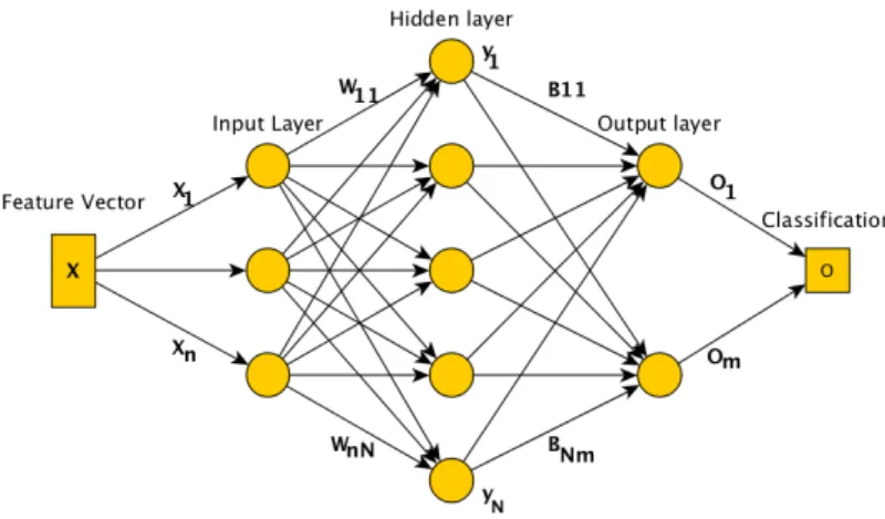
Figure 12: Model for a single hidden layer feedforward neural network.

The very basic artificial neural network (ANN) is the single hidden layer feedforward neural network(SLFN), which structure can be seen in Fig 12. The input layer, the hidden layer and the output layer represent di↵erent nucleus of neurons in the brain. The synapses are represented by the W11 WnN and B11 BnN. These weights are the one that changes during thraining of

the network, the model works as follows:

For n distinct arbitrary samples Xi = (xi1, xi2, ..., xi1d)T 2 <d and m distinct targets

ti = (ti1, ti2, ..., ti1m)T 2 <m with N nodes in the hidden layer. The activation function g is

modeled as: GN(X) = N X i=1 ig(Wi⇤ X + bi) (24)

Here the output weight vector is i = ( i1, i2, ..., iN )T and connects the i-th nodes with the

output nodes. The input weight vector is represented by the Wi= (wi1, wi2, ..., w11d)T, which

connects the input nodes with the i-th hidden node. Lastly the birepresents the threshold of the

i-th hidden node.

Next step is to use a non linear activation function on the GN(X), in order to get the output

from the hidden layer. This is done by the following equation

The final output of the network is a linear combination of all the hidden neurons outputs, according to: Gk = N X i=1 kj⇤ yj ⇤ X + bk (26)

This summation is then submitted to the last activation function and classified according to the last equation.

Ok = ˜g(GN). (27)

Here g(x) and ˜g(x) means that it does not need to be the same activation function.

These types of networks has been shown to be able to approximate complex and nonlinear problems with the help of a back propagation training method. The most common BP algorithm is the descent gradient method, this method starts by initiating the input weight vector W, the output weight vector and the bias vector, b with random values. It will then update these vectors every iteration during the training process, in such a way that the di↵erence between the output vector O and the target vector t moves towards zero. One common error function is the mean squares of errors (MSE), this function has the following structure.

e = 1 m m X k=1 (ok tk)2 (28)

where ok is the actual output response of the network of the k-th output neuron. tk is the

target for the corresponding input value Xn_{, m is the number of outputs. One drawback of this}

training algorithm is that it can get stuck in local minima and never find the true optimal solution, a second drawback is the risk of overfitting. However it is very easy to implement. There has been a lot of research on ANN during the last couple of decades, Huang et al. are some of them [23]. 5.2.7 Bidirectional Recurrent Long Short-Term Memory neural network, BLSTM

NN

A recurrent neural network (RNN) can be seen as an ordinary feedforward network with memory. Where the recurrent part means that there are some neurons that stores the output from some calculating neurons and sends the information back in the next sequence. This means that the information will transmit in two directions, in depth and in time. A bidirectional recurrent network includes a third layer that propagates the information in a sequence backwards.

Changing the ordinary neurons to an LSTM block, the network will be able learn long-term dependencies. Hochreiter and Schmidhuber demonstrate in [19] the superiority over ordinary RNN. 5.2.8 ELM neural network

Two of the drawbacks of the standard SLFN is the training time with an ordinary BP algorithms and that the network can get stuck in some local minima during the training process, which means that it does not find the best working solution [5].

The extreme learning machine (ELM) training technique solves the training time issue by calculating the output weight vector extremely much faster then any ordinary BP algorithm can train the network [16]. The starting point is the same in both cases, the initial values for all weight vectors and all bias values are randomly selected. However instead of iterative updating the di↵erent weight vectors, ELM calculates a new output weight vector, using a generalized inverse matrix. The procedure are as follow. Since Elm uses the same structure as the SLFN described in Figure12, the SLFN equation can be written as

˜ N

X

j=1

jg(wj⇤ Xi+ bj) = oi (29)

Where i = 1, 2, ..., N, j = [ j1, j2, ..., jm]T is the output weight vector connecting the j-th

with the j-th hidden neuron is represented by wj = [wj1, wj2, ..., wjn]T. The bias is represented

by bj of the j-th hidden neuron and oi = [oi1, oi2, ..., oim]T 2 <m is the corresponding output

vector with respect to the input vector xi = [xi1, xi2, ..., xim]T.

In order for this type of neural network to approximate N data samples with zero error, the following equation holds.

˜ N

X

j=1

jg(wj⇤ Xi+ bj) = ti (30)

for i = 1, 2, ..., N. This equation can be written as H = T where H(w1, w2, ..., wN˜, b1, b2, ..., bN˜, x1, x2, ..., xN) = 2 6 6 6 4 g(w1⇤ x1+ b1) g(w2⇤ x1+ b2) · · · g(w_N˜ ⇤ x1+ b_N˜) g(w1⇤ x2+ b1) g(w2⇤ x2+ b2) · · · g(w_N˜ ⇤ x2+ b_N˜) .. . ... . .. ... g(w1⇤ xN + b1) g(w2⇤ xN+ b2) · · · g(wN˜ ⇤ xN + bN˜) 3 7 7 7 5 ˜ N xm = 2 6 6 6 6 6 6 6 6 6 4 T 1 T 2 .. . T ˜ N 3 7 7 7 7 7 7 7 7 7 5 ˜ N xm T = 2 6 6 6 6 6 6 6 6 6 4 tT 1 tT 2 .. . tT N 3 7 7 7 7 7 7 7 7 7 5 N xm

The computation of the output weights in is done according below equation.

= (HTH) 1HTT (31)

Now combining the ide from

5.2.9 Regularized ELM neural network

Since the ELM algorithm aims to draw the error between the target and the output to zero, this can easily create an overfitting solution. This problem can be addressed by adding an weight factor to the calculation of the matrix in Eq31. This factor is know as and introduces the empirical risk that is needed inorder to make sure that the solution is more generalized. The R-ELM’s matrix, is calculated using the following equation.

= (HT_{H +} I₎ 1_HT_{T (32)}

Where I is the identity matrix with the same dimension as H. 5.2.10 FIR-ELM-neural network

Ordinary RNN uses random values for the weights between the nodes. The mostly used training algorithms for these types of neural networks NN, are based on gradient decent approach. The drawback for that is it takes a lot of time to train advanced networks.

2004 Huang et. al. presented the Extreme Learning Machine, ELM, algorithm for neural networks [16]. ELM-neural networks also uses random values for the initial weights, however the

training time are considerably faster, 170 times has been showed in [16]. However this algorithm does not take care of the vanishing problem due to the random weights. 2012 Huang et. al. presented the FIR-ELM-neural network algorithm as a solution to these problems. The initial weights are not randomly set, instead these values are calculated in order to implement a FIR filter [5].

This thesis aims at reducing the residual noise that still can be found in the coefficients by implementing a bandpass filter around the frequencies for the singing voce types bass-soprano. The structure of the FIR-network can be viewed as an ordinary SLFNN with and delay tap, see

Figure 13: Model for a single hidden layer feedforward neural network with time delay nodes representing the di↵erent FIR coefficients.

Figure13, just as an RNN. This is possibly due to the fact that the output of the hidden neurons are the weighted sum of the input signals. This makes that all the di↵erent hidden neurons can be treatable as di↵erent FIR filters. In Figure13the input vector can is X(k) = [x(k)x(k 1)x(k 2)...x(k n + 1)]T _{and the output vector can be expressed as O(k) = [o}

1(k)o2(k)...om(k)].

With this notation the output from the hidden neuron is expressed as: yi(k) = n X j=1 wijx(k j + 1) = WiTX(k) (33) Where Wi= [wi1wi2...win]T, f ori = 1, 2, ..., ˜N

The output takes the form of:

oi(k) = ˜ N X p=1 piW_pTX(k) (34)

for i= 1, 2, ..., m. The output vector takes the form

O(k) = ˜ N X p=1 pWpTX(k) (35) and i = [ i1 i2... im]T, for i = 1, 2, ..., ˜N .

When training the network, all N distinct dublets (xi, ti) are expresses as

Xi= [xi1xi2...xin]T (36)

ti= [ti1ti2...tim]T (37)

thus the output vector Oi is of the form

Oi = ˜ N X p=1 pWpTXi(k) (38)

These N equations can be written in a compact way as

H = O (39) where H = 2 6 6 6 4 w1x1 w2x1 · · · w_N˜x1 w1x2 w2x2 · · · w_N˜x2 .. . ... . .. ... w1xN w2xN · · · w_N˜xN 3 7 7 7 5 ˜ N xm = 2 6 6 6 6 6 6 6 6 6 4 T 1 T 2 .. . T ˜ N 3 7 7 7 7 7 7 7 7 7 5 ˜ N xm O = 2 6 6 6 6 6 6 6 6 6 4 oT 1 0T 2 .. . oT N 3 7 7 7 7 7 7 7 7 7 5 N xm

Now reusing the equation32from the R-ELM algorithm, the output weight matrix for the FIR-ELM network can be computed in an robust way.

5.3

Design

Two di↵erent approaches will be conducted during this thesis work in order to decompose the audio signal into estimations of singing and instrumental accompaniment.

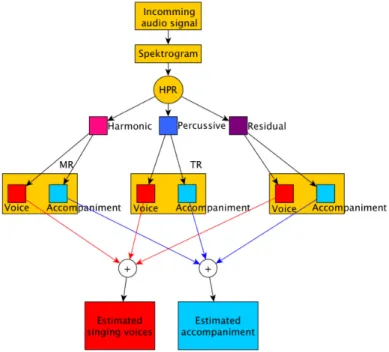
Firstly, this thesis will follow and aim at enhancing the work previously performed by Driedger et al. in [1] in order to separate the singing component from the instrumental component of the audio signal. The architecture for this approach looks like the one in Fig14. In the top layer, the incoming signal will be divided into three di↵erent blocks using the Harmonic-Percussive-Residual method (HPR). The HPR-algorithm is described in more detail in section 5.2.1.

The first output from HPR contains the harmonic components of the audio signal, and will be referred as the Melody-Residual (MR) block. These components reflect the cleanest parts of voices as well as some instrumental tones. The Harmonic block will be further decomposed into two sub blocks, harmonic singing voice and harmonic accompaniment. The MR block is further described in section 5.2.2.

The second block in the HPR is the Percussive block. Here are the most striking sound fre-quencies. Voice fricatives will be found here, and the decomposition of this block is examined in Section 5.2.3.

In section 5.2.4, the last block, the residual block will be explored. The elements that do not clearly belong to the harmonic or the percussive block will be located here. In [1] these components

Figure 14: Model for the cascaded audio decomposition using HPR.

are selected using a single separation variable. I propose that a second separation variable shall be introduced in order to let di↵erent amounts of components from the two main blocks contribute in a more appropriate way to the residual block.

The output from all of these sub blocks will merge in two di↵erent blocks. The first block will contain the estimation of the singing voice. The second block, contains the estimated accompani-ment, see Fig14.

Secondly, in this thesis the pre-processing step uses the same HPR algorithm in both approaches. For feature extracting this approach will take advantage of the powerful Mel Frequency Cepstrum Coefficients technic, see section 5.2.5. For classifier, a Long Short-Term Memory (LSTM) neural network will be implemented in order to divide the singing voice components and the accompani-ment components. Simon Leglaive et al. showed in [4] that it is possibly to show the presence of singing voices in the audio signal. See Fig15for a overview of the working model.

Concerning the voice type classification, a finite impulse response extreme learning machines (FIR-ELM) neural network will be used. Khoo et al. showed in [5] very good results in classifying Chinese folk songs using this type of neural network. The construction of this type of network will be explained in section 5.2.10.

5.4

Audio samples

In the beginning to the middle of this project, this thesis author searched the internet for a predefined music set with a cappella opera songs. This turned out to be quiet hard to find. The author only found training sets with Chines opera music. Chinese and western singing voices do not match [6] and it was decided that these music sets was to be discarded. The training set and the validation set there for had to be recorded from internet.

The sample sets for training and validation, constitutes the 7 basic voice types: • Soprano

• Mezzo-soprano • Contralto • Countertenor

Figure 15: Model for audio decomposition using a HPR and a Bidirectional recurrent neural network.

• Tenor • Baritone • bass

Where the three first are the classes with highest frequencies band and are most often considered for female singing voices.

In the training set each voice type are represented by 5 di↵erent vocalists randomly selected from di↵erent internet pages [27–33]. These pages has either a list of famous names or a list of famous roles. In each case the name or the roll has then been searched for on YouTube in order to find a good enough quality and then recorded in a Matlab program. The recorded quality is 16 bits, sample rate is 40960 Hz and each recorded sung was 30 seconds long. From these 30 seconds all parts where there are only accompaniment are manually removed. After making sure that all voice types has the equal amount of samples, there are 65 samples left for each voice type, each containing 1 second of audio music this gives a total of 455 samples to use for the feature extraction block.

The evaluation dataset contains recorded audio from the “finale” of Medea with two singers, Maria Callas and one male singer [34]. This dataset is produced in a similar way as the above datasets. The recording with Maria Callas is 2 min and the male singer is recorded for 45 seconds, after manually removing the music sections with only accompaniment the evaluation dataset that has been used contains 56 numbers of Maria Callas samples and 24 samples that do not belong to her. Each 1 second long.

6

Results and Discussions

The result from the multilayer decomposition showed that it was feasibly to classify the soprano singing voice type. And since the BLSTM RNN was not implemented, the single layer architecture used a FIR-ELM network without the SL blocks coefficients and the estimation of voice activity was made manually.

6.1

Experiment setup

In order to test the feasibility of classifying the singing voice type with an FIR-ELM network first the type, coefficients and the order of the FIR filter has to be decide. Since the filter should reduce the e↵ect of all voice types except for the soprano type and also the accompaniment that the previous HPR algorithm has mismatched. The filtertype has been decide to be a bandpass filter. The low-cuto↵ frequencies for all the input weights are 435 Hz, this is five times lager then the fundamental frequency for the bass type but only twice the fundamental frequency of the soprano type. The high cuto↵ frequencies are 5235 Hz, which corresponds to five times the highest fundamental frequency in the soprano range. Second, the structure of the network has to be created. The amount of nodes in the hidden layer is set to 4. Test runs in the implementation phase of the ELM algorithm with 20, 200 and 2000 hidden nodes gave similar result, however it was an huge di↵erence in the calculation time. So the amount of hidden neurons in the FIR-ELM structure was set to the same number of FIR coefficients, 4. There are four test cases. The di↵erent

Separation factor Test values

Harmonic first iteration 1.0 1.1 1.1 1.2 1.2 1.1 1.0 1.0 Percussive first iteration 1.0 1.0 1.1 1.0 1.1 1.2 1.2 1.3 Harmonic second iteration 1.0 1.0 1.0 1.0 1.0 1.0 1.0 1.0 Percussive second iteration 1.0 1.0 1.0 1.0 1.0 1.0 1.0 1.0 Table 1: Separation factors for the HPR decomposition that are tested in this thesis.

test scenarios are dependent on the two median filters and the di↵erent separations factors in the HPR decomposition, the horizontal median filter values are 500 Hz and 1000 Hz. While the vertical median filters are 200 ms and 400 ms. Each test has 8 di↵erent separation factors combinations, the combinations can be seen in Table1. The size of this test set is heavily constrained to time. Each test took around 9 hours to complete.

6.2

Result for research question 1

As can be seen in tables2 – 5, for both systems, the single layer decomposition system and the multilayer decomposition system it is feasibly to classify the soprano voice type in general. Very small di↵erences can be observed in the classification result regarding the di↵erent sizes of the median filters. However it can be seen that the result tends to be more accurate when the two separation factors are more equal.

6.3

Result for research question 2

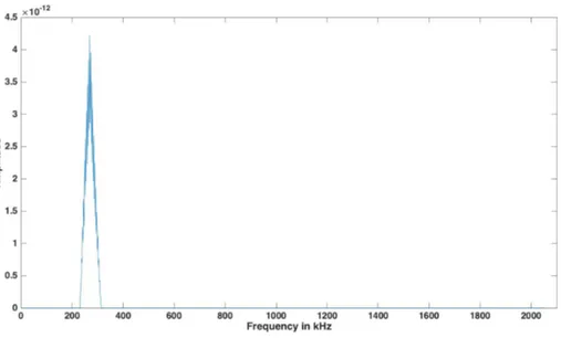
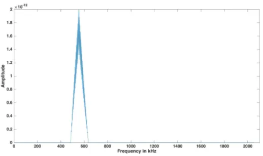
The author of this thesis could not hear any improvement in the sound quality that could lead to the conclusion that a second separation factor would improve the HPR algorithm for now. This statement can also be confirmed by observing Figure16. The figure shows the result after test 1 and test 4. di↵erences are to small, however they are there.

6.4

Result for the hypothesis

This study confirmed that it is feasibly to classify the soprano singing voice type when Maria Callas performs the parts of the classical Greek tragedy Medea. The systems classified correctly with 98.5% accuracy in the evaluation dataset for both systems.

Single layer/ multilayer

architecture Result in percent

Training single 63.480 63.459 63.419 63.419 63.419 63.419 63.419 63.419 Test single 74.944 74.939 75.180 75.183 75.183 75.183 71.183 71.183 Training multi 63.432 63.432 63.391 63.378 63.405 63.412 63.419 63.419 Test multi 75.119 75.119 75.160 75.119 75.132 75.142 75.183 75.183 Table 2: The result from test 1: Horizontal median filter = 500 Hz, Vertical median filter 200 Hz.

Single layer/ multilayer

architecture Result in percent

Training single 63.419 63.466 63.419 63.419 63.419 63.419 63.419 63.419 Test single 75.183 74.967 75.183 71.183 71.183 75.183 75.183 75.183 Training multi 63.419 63.432 63.391 63.378 63.405 63.412 63.419 63.419 Test multi 75.183 75.119 75.160 75.119 75.132 75.142 75.183 75.183 Table 3: The result from test 2: Horizontal median filter = 500 Hz, Vertical median filter 400 Hz.

Single layer/ multilayer

architecture Result in percent

Training single 63.419 63.419 63.419 63.419 63.419 63.419 63.419 63.419 Test single 75.183 75.183 75.183 71.181 71.181 75.183 75.183 75.183 Training multi 63.419 63.419 63.400 63.391 63.425 63.419 63.419 63.419 Test multi 75.183 75.183 75.183 71.186 71.181 75.183 75.183 75.183 Table 4: The result from test 3: Horizontal median filter = 1000 Hz, Vertical median filter 200 Hz.

Single layer/ multilayer

architecture Result in percent

Training single 63.419 63.419 63.419 63.419 63.419 63.419 63.419 63.419 Test single 71.183 71.183 71.183 71.181 71.181 71.183 71.183 71.183 Training multi 63.419 63.419 63.419 63.419 63.419 63.419 63.419 63.419 Test multi 75.183 75.183 75.183 71.165 71.165 75.183 75.183 75.183 Table 5: The result from test 4: Horizontal median filter = 1000 Hz, Vertical median filter 400 Hz.

Figure 16: The blue graph is the estimated voices after test 1 and the orange colored graph is the result after test 4. As can be seen the overall pattern are very similar, however the amplitude changes.

7

Conclusion

In this thesis two classification systems were implemented using the FIR-ELM algorithm, both using the HPR decomposition technique as base algorithm for segmenting the singing voices and the accompaniment. The first system only uses the Harmonic- and the percussive output from the HPR decomposition and extracts the MFCC from these blocks in order to classify the singing voice types. The second system decompose the three outputs from the HPR algorithm in one more level and then combine the results into one estimated singing voice audio signal. From this estimation, the extraction of the Mel Frequency Cepstral Coefficients takes place, and the classification of the singing voice type soprano takes place.

Both systems showed that the HPR decomposition technique can be used in order to decom-pensate western opera music, and also that it is feasibly to use the FIR-ELM training technique in order to classify classic singing voice types as Soprano or non-soprano. However, further test and calibration of the amount of the FIR coefficients needs to be done if any one of the systems should work robust in a live performance. With only 4 hidden neurons in each network, the results are quite satisfactory.

8

Outcome

This thesis work aims at developing two singing recognitions systems.

One system that uses a multilayer architecture for the audio decomposition in order to classify the singing voice type. The second system takes advantage of single layer architecture in the audio decomposition and then uses a Long Short-term neural network as singing voice classifier. The output from both systems shall be used as input for a voice type classification system, this classification system in made of a FIR-ELM-neural network. Two system will be evaluated, Firstly, one with ordinary RNN. Secondly, one system with LSTM blocks instead of ordinary perceptron entities. Further more a comparison between the four systems will be conducted.

9

Future work

There are a lot that can be improved on these systems. Firstly, the parameters for the HPR decomposition can be improved using an optimized generic algorithm. Secondly, the quality on the estimated voices can be improved by post processing the di↵erent blocks in the HPR decomposition, this should lead to a better subjective singing voice type recognition. Thirdly, the singing voice recognition part was not successfully implemented due to that the author did not find any suitably existing opera a cappella training set. One way to work from here is to use now existing singing voice type training set and from that developed an singing recognition system. Also the Long Short-term network node needs to be implemented with the ELM structure in mind.

References

[1] Driedger, Jonathan, and Meinard Muller. ”Extracting singing voice from music recordings by cascading audio decomposition techniques.” Acoustics, Speech and Signal Processing (ICASSP), 2015 IEEE International Conference on. IEEE, 2015.

[2] Huang, Po-Sen, et al. ”Singing-voice separation from monaural recordings using robust prin-cipal component analysis.” 2012 IEEE International Conference on Acoustics, Speech and Signal Processing (ICASSP). IEEE, 2012.

[3] Liutkus, Antoine, et al. ”Adaptive filtering for music/voice separation exploiting the repeating musical structure.” 2012 IEEE International Conference on Acoustics, Speech and Signal Processing (ICASSP). IEEE, 2012.

[4] Leglaive, Simon, Romain Hennequin, and Roland Badeau. ”Singing voice detection with deep recurrent neural networks.” 40th International Conference on Acoustics, Speech and Signal Processing (ICASSP). 2015.

[5] Khoo, Sui Sin. ”The Single Hidden Layer Neural Network Based Classifiers for Han Chinese Folk Songs.”

[6] Tang, Zheng, and Dawn AA Black. ”Melody Extraction from Polyphonic Audio of Western Opera: A Method based on Detection of the Singer’s Formant.” ISMIR. 2014.

[7] Ono, Nobutaka, et al. ”Separation of a monaural audio signal into harmonic/percussive com-ponents by complementary di↵usion on spectrogram.” Signal Processing Conference, 2008 16th European. IEEE, 2008.

[8] Driedger, Jonathan, Meinard Mller, and Sascha Disch. ”Extending Harmonic-Percussive Sep-aration of Audio Signals.” ISMIR. 2014.

[9] Fitzgerald, Derry. ”Harmonic/percussive separation using median filtering.” (2010).

[10] Virtanen, Tuomas, Annamaria Mesaros, and Matti Ryynnen. ”Combining pitch-based infer-ence and non-negative spectrogram factorization in separating vocals from polyphonic music.” SAPA@ INTERSPEECH. 2008.

[11] Ryynnen, Matti P., and Anssi P. Klapuri. ”Automatic transcription of melody, bass line, and chords in polyphonic music.” Computer Music Journal 32.3 (2008): 72-86.

[12] Talmon, Ronen, Israel Cohen, and Sharon Gannot. ”Transient noise reduction using nonlocal di↵usion filters.” Audio, Speech, and Language Processing, IEEE Transactions on 19.6 (2011): 1584-1599.

[13] Cohen, Israel. ”Noise spectrum estimation in adverse environments: Improved minima con-trolled recursive averaging.” IEEE Transactions on speech and audio processing 11.5 (2003): 466-475.

[14] [online] avaible: 2016-08-11: https://se.mathworks.com/matlabcentral/fileexchange/55030-

speech-enhancement-based-on-student-t-modeling-of-te-operated-pwp-coefficients/content/StudentTTeagerBasedSpeechEnhance/omlsa.m

[15] Michael Nenevitsky, ”Artificial Intelligence a guide to intelligent systems”, Addison Wesley, 2011, third edition.

[16] Huang, Guang-Bin, Qin-Yu Zhu, and Chee-Kheong Siew. ”Extreme learning machine: a new learning scheme of feedforward neural networks.” Neural Networks, 2004. Proceedings. 2004 IEEE International Joint Conference on. Vol. 2. IEEE, 2004.

[17] Huang, Gao, et al. ”Trends in extreme learning machines: a review.” Neural Networks 61 (2015): 32-48.

[18] Thielscher, Michael, and Dongmo Zhang, eds. AI 2012: Advances in Artificial Intelligence: 25th International Australasian Joint Conference, Sydney, Australia, December 4-7, 2012, Proceedings. Vol. 7691. Springer, 2013.

[19] Hochreiter, Sepp, and Jrgen Schmidhuber. ”Long short-term memory.” Neural computation 9.8 (1997): 1735-1780.

[20] Poria, Soujanya, et al. ”Fusing audio, visual and textual clues for sentiment analysis from multimodal content.” Neurocomputing 174 (2016): 50-59.

[21] Logan, Beth. ”Mel Frequency Cepstral Coefficients for Music Modeling.” ISMIR. 2000. [22] Huang, Po-Sen, et al. ”Singing-voice separation from monaural recordings using robust

prin-cipal component analysis.” Acoustics, Speech and Signal Processing (ICASSP), 2012 IEEE International Conference on. IEEE, 2012.

[23] Huang, Guang-Bin, Lei Chen, and Chee-Kheong Siew. ”Universal approximation using in-cremental constructive feedforward networks with random hidden nodes.” Neural Networks, IEEE Transactions on 17.4 (2006): 879-892.

[24] [online] avaible: 2016-05-11: http://www.zainea.com/voices.htm [25] [online] avaible: 2016-04-22: https://en.wikipedia.org/wiki/Ear [26] [online] avaible: 2016-04-26: http://www.multimed.org/singing/

[27] [online] avaible: 2016-04-27: https://en.wikipedia.org/wiki/Category:Operatic sopranos [28] [online] avaible: 2016-04-27: https://en.wikipedia.org/wiki/Mezzo-soprano

[29] [online] avaible: 2016-04-27: https://en.wikipedia.org/wiki/List of operatic contraltos [30] [online] avaible: 2016-04-27: https://en.wikipedia.org/wiki/Countertenor

[31] [online] avaible: 2016-04-27: https://en.wikipedia.org/wiki/Tenor

[32] [online] avaible: 2016-04-27: http://www.thetoptens.com/male-bar-tones/

[33] [online] avaible: 2016-04-27: http://wwwnicholashay-operahistorian.blogspot.se/2013/09/ten-great-operatic-basses.html

[34] [online] avaible: 2016-09-06: https://www.youtube.com/watch?v=FptWaSW-siQ

[35] wan, Pawe, et al. ”Automatic singing voice recognition employing neural networks and rough sets.” Rough Sets and Intelligent Systems Paradigms. Springer Berlin Heidelberg, 2007. 793-802.

[36] Huang X, Acero A, Hon H, (2001), Spoken Language Processing: A guide to theory, algorithm, and system development, Prentice Hall. Upper Saddle River, Nj, USA (pp. 314-215).