Does infrastructure really cause growth? : the time scale dependent causality nexus between infrastructure investments and GDP

Does Infrastructure Really Cause Growth?

The Time Scale Dependent Causality Nexus between

Infrastructure Investments and GDP

Niclas A. Krüger – VTI CTS Working Paper 2012:15

Abstract

This paper investigates the relationship between infrastructure investments and economic activity in Sweden for the period 1800-2000. In order to overcome the problem of endogeneity, independent time scales are used to analyze the relationship. The paper also examines the dynamics between the variables by testing for causality in the Granger sense and constructing a vector autoregressive model separately for each time scale. The finding is that the causality nexus between growth and transport infrastructure investment is time-scale-dependent since it reverses in a comparison of the short-run dynamics (2-4 years) and the longer-run dynamics (8-16 years). This causality reversal is unique for infrastructure investments compared to investments in other sectors of the economy.

Keywords: Infrastructure, GDP growth, Investment, Time scale decomposition

JEL Codes: E22, E32, N7

Centre for Transport Studies SE-100 44 Stockholm

Does Infrastructure Really Cause Growth?

The Time Scale Dependent Causality Nexus between

Infrastructure Investments and GDP

Niclas A. Krüger a,b,c a

Centre of Transport Studies, Stockholm b

Swedish National Road and Transport Research Institute c

Swedish Business School, Örebro University Phone: +46 70 33 54 599

E-mail: niclas.kruger@vti.se

Abstract: This paper investigates the relationship between infrastructure investments and economic activity in Sweden for the period 1800-2000. In order to overcome the problem of endogeneity, independent time scales are used to analyze the relationship. The paper also examines the dynamics between the variables by testing for causality in the Granger sense and constructing a vector autoregressive model separately for each time scale. The finding is that the causality nexus between growth and transport infrastructure investment is time-scale-dependent since it reverses in a comparison of the short-run dynamics (2-4 years) and the longer-run dynamics (8-16 years). This causality reversal is unique for infrastructure investments compared to investments in other sectors of the economy.

Keywords: Infrastructure, GDP growth, Investment, Time scale decomposition JEL Code: E22, E32, N7

1 Introduction

The relationship between infrastructure capital and economic growth has been

studied in a vast range of papers and become a controversial issue. A number of

empirical studies have found very high returns to infrastructure investment,

starting with Aschauer (1989), who uses a standard production function

augmented by public capital and concludes that the decrease in infrastructure

investments might be an explanation for the productivity slowdown in the United

States since the 1970s. However, his results have been questioned in other

empirical studies and surveys (Gramlich, 1994; Munnell, 1992). While

infrastructure may lead to higher productivity and output, past and current

economic growth also increases the demand for infrastructure services and

thereby induces increased supply. Accordingly, some studies find that the

causality direction is from GDP to infrastructure rather than the other way around

(Gramlich 1994; Munnell 1992). Therefore, it is not sufficient to establish an

empirical link between GDP and infrastructure investments; the problem of the

causal direction between economic growth and infrastructure investment has to

be explicitly addressed. It might well be the case that high GDP and high

infrastructure investments are correlated, but that there is no causal relationship,

which has important implications for public policy.

There are two major problems when estimating the impact of infrastructure

on growth. When analyzing long-term variations, it is evident that there are

common trends in aggregate production and infrastructure, but, when analyzing

investment spending, even if unproductive, directly boosts GDP. This makes it

difficult to test for causality using conventional methods. In order to overcome

these problems we use time-scale decomposition to filter trend behaviour and

short-term effects from the data. We test for causality in the Granger (1969)

sense in a multi-equation time-series framework. The idea is that unexpected

shocks in one variable should help us forecast shocks in another variable in order

to establish a causal relationship, independent from the lead-lag relationship

between expected regular movements in the variables. Granger-causality tests are

typically carried out in either vector auto-regression models (VAR) or vector

error correction models (VECM). In a VAR-model each variable is regressed on

its own lags and on lags of the other variables, meaning that all variables are

treated as jointly determined. This implies that no ex ante causality direction is

imposed. Given that we do not have a theory about the timing of the

infrastructure investment process, a VAR model is clearly appropriate here, since

we do not restrict data in order to fit any structural model. Our study is not

concerned with the analysis of the determinants of economic growth, but

addresses the statistical causal relationship between GDP and a broad aggregate

of infrastructure investments. This is per se nothing new; for instance, King et al

(1991) estimate a VAR for output, consumption and investment. The novelty

here is that we use time-scale decomposition of economic growth and

investments to address the problems that have materialized in previous studies.

As we are of the opinion that only time-scale decomposition can disentangle the

first empirical test of causality between infrastructure investments and GDP

based on wavelet analysis. Since we are mainly interested in the time time-scale

decomposition properties of wavelets, we do not compare wavelet-based

techniques with more common time series techniques as for example spectral

analysis.

Wavelet methods transform a time series into several time series which

reflect properties of the original time series for different time scales. Using

different time scales is quite common in economics, since we usually analyze

relationships between variables using daily, monthly or yearly data. In wavelet

analysis, however, the information contained in one time scale is independent

(orthogonal) of the information contained in the other time scales. Hence, the

transformed time series may be added together to get the original time series,

which implies that the transformed series essentially contain the same

information as the original time series. Wavelet decomposition allows us to

perform an analysis of variance (ANOVA) and covariance across time scales.

Using the wavelet method is like sliding magnifying glasses of different power

over the time series in order to see different levels of detail. Looking at the finest

scales (highest magnification), we cannot see the whole picture, whereas looking

at the coarsest scales (lowest magnification) to see the whole picture, we lose

information about the details. With a Wavelet method there is no need to make

any trade-offs since the different scales may be examined simultaneously. Thus,

changes in local trends separately in order to disentangle the relationship between

investments and GDP across different time scales.

Studies using data covering long periods of time are very rare. Luoto (2011)

examines Finnish land and water construction investments series for 1860-2003,

finding that investment in infrastructure capital had a strong positive effect on

output growth over the long-run. This paper uses a new long run data set on

infrastructure capital formation in Sweden during the nineteenth and twentieth

century. Sweden is and has been an open economy highly integrated in

international markets, which implies that shocks to the economy are often

exogenous. We use data obtained from Edvinsson (2005) for Swedish GDP and

investments in the transport and communication sector for the period 1800–2000.

During that period Sweden underwent the industrial revolution and large

infrastructure projects were carried out. For example, the construction of a

national railway network started in the 1860s. Sweden has a small population and

comprises a large area; the maximum north-south distance is 1,574 kilometres

and the maximum east-west distance is 499 kilometres. Therefore, it seems

reasonable to conclude that these infrastructure investments connected markets in

different Swedish regions, which had previously been separated, and thereby

promoted growth. Since spatial integration takes time and the resulting effects on

production probably take even more time, there is no ex-ante preferable time

scale we want to analyze. A time-scale decomposition, which lets the data speak

analysis compared to either traditional analysis or to the extraction of business

cycles with the more common Hodrick-Prescott filter.2

Data limitations have previously forced economists to use public investment

expenditures as a proxy for total infrastructure investment (Gramlich, 1994).

Public investment, however, often consists of not only infrastructure investments

but also residential investments and spending on public buildings. In Sweden,

both presently and historically, part of the infrastructure is financed and initiated

by the private sector. Our data captures both public as well as private

infrastructure investments, thus providing a better picture of the relationship

between growth and infrastructure in general. Instead of focusing on railroads or

roads on a disaggregate level, we analyze the aggregated transport and

communications sector. Transport and communications are closely related, and

recent studies show that both infrastructure usage (travel) and telecommunication

services satisfy a basic need for mobility, thus being substitutes for and/or

complements to each other (for an overview, see Mokhtarian and Salomon,

2002).

This paper is structured as follows. Section 2 outlines the methodology used

in our analyses and section 3 contains the results. We find that the causality

nexus between growth and transport infrastructure investment is time-scale

dependent since it reverses in a comparison of the short-run dynamics (2-4 years)

and the longer-run dynamics (8-16 years). This causality reversal is unique for

2

More technically, since the Hodrick-Prescott filter is based on minimization of a function, it is likely to introduce spurious cycles.

infrastructure investments compared to investments in other sectors in the

economy. The discussions in section 4 conclude the paper.

2 Method: Wavelet decomposition

A time series is usually analyzed either in the time domain or in the frequency

domain. The Fourier transform serves as a connection between time series

analyses in the time domain and the frequency domain. Fourier transformations

use a sum of sine and cosine functions with different frequencies and

amplitudes.3 Since sine and cosine functions have a repeating pattern of

amplitudes along the time axis, these Fourier transformations are not applicable

to time series with structural breaks or sharp peaks. A Wavelet transformation is

similar to a Fourier transformation in that it converts the time series from the

time domain to the frequency domain. In wavelet analysis, though, the amplitude

for a given frequency can change across time.

A wavelet is defined as any real valued function f over the real axis,

satisfying the following two basic properties:

( )

∫

( )

∫

The first property makes sure that positive and negative deviations from zero

cancel out so that the basic definition of a wave is satisfied. The second property

3

One Fourier transform is -i x

-F( ) =ϖ ∞f(t)e ω dt

∞

∫

iy

makes sure that the deviations from zero are limited to a relatively small interval

in time (in contrast to a sine-wave, which starts at negative infinity and goes to

positive infinity). We therefore have a ‘small wave’, which is the literal meaning

of ‘wavelet’. There are several other properties a wavelet has to have in order to

be of any practical use; the most important is the so-called admissibility property

(for details see Percival and Walden, 2000).

A discrete wavelet transformation (DWT) decomposes a time series into

different frequency bands. In wavelet analysis each frequency band is called a

scale. The first scale λ1 covers the frequencies 1 4 to

1

2 and scale λj the

frequencies 1₁

2j + to 1

2j , so that the width of each frequency band is scale

dependent. A wavelet transformation with J-scales produces J sets of wavelet

coefficients and one set of scaling coefficients. The wavelet coefficients can be

interpreted as weighted differences on the physical scale λj = 2 j−1

∆t, thus

representing high frequency changes. Since the wavelet filter approximates an

ideal band pass filter with pass band [1/2j+1, 1/2j], the λj scale wavelet coefficients

show variations with a period in the interval between 1/2j+1 and 1/2j (Gallegati,

2007). The scaling coefficients can be interpreted as the sum of weighted

averages, thus representing low frequency changes in local means. The different

wavelet scales are an orthogonal transform of the original time series, meaning

that we can easily reconstruct the time series from its transform. Thus, the

‘information’ in the transform is equivalent to the ‘information’ in the original

A practical shortcoming of DWT is that only2J observations, where J is an integer, can be included in the analysis. Further, the decomposition is dependent

on both the specific choice of wavelet function and the starting point on the time

axis. These deficiencies may be addressed by using a variant of DWT called the

maximum overlap discrete wavelet transformation (MODWT) as described in

Percival and Walden (2000). MODWT uses an overlapping window algorithm to

circumvent the2J

-restriction, and decreases sensitivity with respect to choice of

wavelet function and starting point. Figure 1 illustrates the time-scale

decomposition of GDP using four different time scales, generating four sets of

wavelets (W1-W4) and one set of scaling filter coefficients (V4).

One convenient property of a wavelet transform is the so-called energy

preservation across time scales. For a MODWT transform it can be shown that

the following relationship holds:

∑

∑

∑

where xt is the data value and wj,t and vt are the wavelet coefficients and scaling

coefficients, respectively. An unbiased estimator of the wavelet variance is

(Gencay et al, 2002):

∑

Figure 1: Wavelet time scale decomposition for GDP (growth rates)

Hence, the variance of the original time series can be decomposed into the sum

of the variances over different time scales. This property allows us to perform an

analysis of variance (ANOVA) across time scales. Analogously, we may define

the wavelet covariance for two time series, thus enabling us to decompose the

relation between two variables on a scale by scale basis. Based on the wavelet

of the original time series, producing a series of wavelet details and a wavelet

smooth. For a MRA based on MODWT the following relationship holds:

∑

where xt is the value of the time series at time t and dj,t and st are the wavelet

details and wavelet smooth, respectively. Hence, each data point can be

decomposed as the sum of the wavelet details and the wavelet smooth over

different time scales. The smooth coefficients mainly capture the underlying

trend behaviour of the data on the coarsest scale, while the details coefficients

represent deviations from the trend behaviour for increasingly finer scales. MRA

is therefore a convenient way of performing analysis based on levels rather than

variances for different time scales.

3 Analysis

3.1 Data

Sweden has a long tradition of demographic and economic statistics.

Tabellverket, founded in 1749 with the task of registering Swedish demographic

data, was succeeded in 1858 by Statistiska Centralbyrån. Sweden is the only

country, besides Finland (a former part of Sweden), that has maintained

continuous population data since 1749. The first attempt to construct consistent

historical national accounts for Sweden was published in 1937 as National

Income of Sweden 1861-1930, written by Erik Lindahl, Einar Dahlgren and Karin

relationship between economic conditions and mortality for the period 1865 to

1913. In 1956 Olof Lindahl extended the data series up to 1951 (Lindahl, 1956)

and in 1967 Östen Johansson presented a GDP series for 1861-1955 (Johansson,

1967). A series named Swedish Historical National Accounts (SHNA), under the

shared leadership of Olle Krantz and Lennart Schön and published between 1986

and 1995, contains annual data over the production of different activities for the

period 1800-1980 (for detailed references, see Edvinsson, 2005). New

calculations in Edvinsson (2005) for the period 1800-2000 are based on the

SHNA-series data and, unlike the SHNA-studies, the data for GDP and its

composition are extrapolated backwards from modern day data maintained by

Statistics Sweden in accordance with modern standards of national accounting.

The analysis in this paper is conducted using annual data for nominal

investment expenditures in purchaser prices for the transport and communication

sector, including a series of consumption of fixed assets, a purchase price index

for investment expenditures, population data and real GDP growth per capita for

Sweden for the period 1800-2000. The data used is based on Edvinsson (2005)

and retrieved via www.historia.se. Figure 2 shows nominal GDP and investment

Figure 2: GDP and infrastructure investments (log nominal levels)

3.2 Data analysis

Growth rates are calculated as the first difference of the log-transformed time

series for infrastructure investments and for real GDP. For the whole period the

mean GDP growth rate was 1.7 percent (mean deviation 3.6 percent) and the

mean investment rate in transport and communication was 2.9 percent (mean

deviation 22.9 percent). We decompose the two transformed series (see Figure 3)

−5 0 5 10 Investment 5 10 15 GDP 1800 1850 1900 1950 2000 t GDP Investment

into their timescale components using the maximum overlap discrete wavelet

transform (MODWT).

The wavelet filter used in the decomposition is the Haar-filter of length

L=2, with periodic boundary conditions.4 The Haar-filter has the shortest

possible filter length and is symmetric. The short filter length ensures the lowest

possible influence of the periodic boundary condition. The application of the

wavelet transform with a number of scales J = 4 produces four sets of wavelets

and one set of scaling filter coefficients (see Figure 4).

Figure 3: GDP and infrastructure investments (per capita growth rates)

4

The coefficients generated by MODWT are affected by the boundary condition at the beginning and the end. If the filter is of length L, (2j-1)(L-1) coefficients are affected for scale j, whereas (2j-1)(L-1)-1 beginning and (2j -1)(L-1) ending details and smooth coefficients are affected (Percival and Walden, 2000). Another source of spurious correlation is potentially the shape of the wavelet used. Therefore, the smoothness of the wavelet function used should resemble the underlying data. The relative roughness of the Haar-wavelet seems suitable when analyzing growth rates (see Figure 3 and Figure 4).

Using annual data scale 1 represents 2-4-year period dynamics, while scales 2, 3,

and 4 correspond to 4-8, 8-16 and 16-32-year period dynamics, respectively.

With wavelet analysis we can decompose the total covariance in a bivariate

relationship on a scale by scale basis and thereby determine to what extent each

scale contributes to the overall association between the two variables. The results

of the correlation analysis for net infrastructure investments and GDP are shown

in Table 1. −1 −.5 0 .5 1 1.5 Gross investment −.1 −.05 0 .05 .1 .15 GDP 1800 1850 1900 1950 2000 t GDP Gross investment −1 0 1 Net investments −.1 −.05 0 .05 .1 .15 GDP 1800 1850 1900 1950 2000 t GDP Net investments

−.5 0 .5 1 D1 Inv −.1 −.05 0 .05 D1 GDP 1800 1850 1900 1950 2000 t D1 GDP D1 Inv −.4 −.2 0 .2 .4 .6 D2 Inv −.04 −.02 0 .02 .04 .06 D2 GDP 1800 1850 1900 1950 2000 t D2 GDP D2 Inv −.2 −.1 0 .1 .2 D3 Inv −.02 −.01 0 .01 .02 D3 GDP 1800 1850 1900 1950 2000 t D3 GDP D3 Inv −.1 −.05 0 .05 D4 Inv −.01 −.005 0 .005 .01 D4 GDP 1800 1850 1900 1950 2000 t D4 GDP D4 Inv

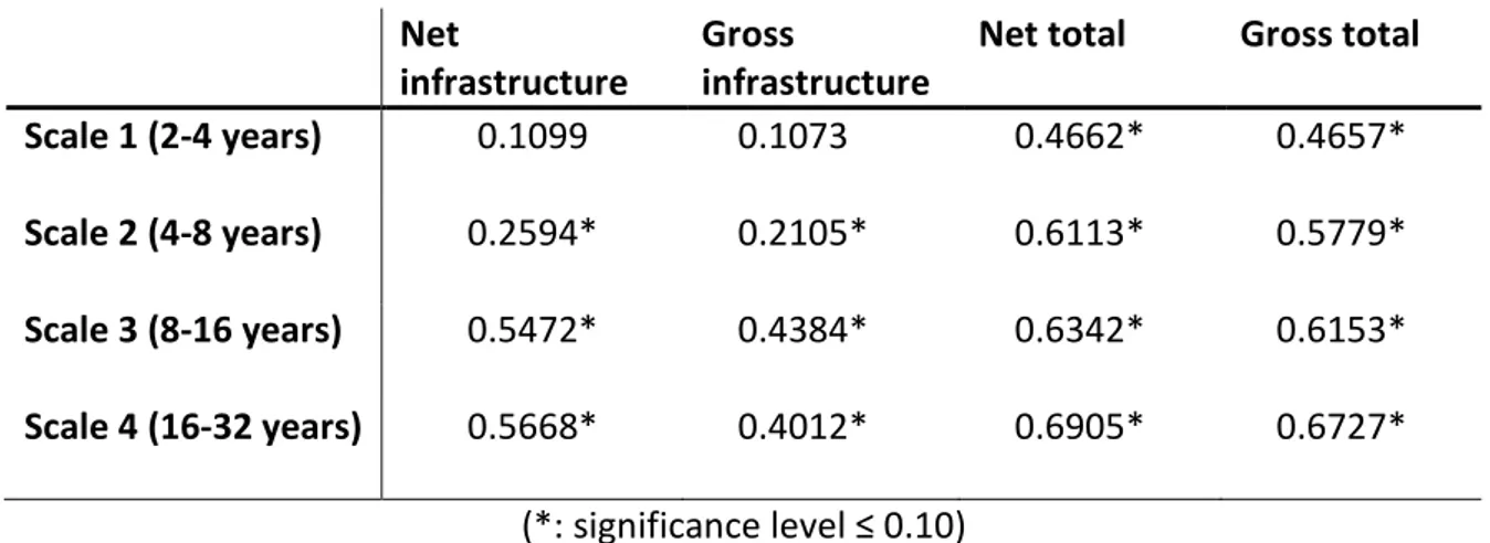
Table 1: Correlation net infrastructure investments and GDP 1800-2000

We can see that the correlation between growth and transport investments

increases with the length of the time scale. In the short term the correlation is

weak and insignificant, whereas the degree of association increases with the

time scale. The results seem reasonable since infrastructure investment

planning often take years from initiation to execution.

Table 2 compares the correlation between net and gross investments and

between infrastructure investments and total investments in the economy.

Table 2: Comparison correlation coefficients GDP & investments Net

infrastructure

Gross

infrastructure

Net total Gross total Scale 1 (2-4 years) 0.1099 0.1073 0.4662* 0.4657* Scale 2 (4-8 years) 0.2594* 0.2105* 0.6113* 0.5779* Scale 3 (8-16 years) 0.5472* 0.4384* 0.6342* 0.6153* Scale 4 (16-32 years) 0.5668* 0.4012* 0.6905* 0.6727*

(*: significance level ≤ 0.10)

The correlation structure is similar for net and gross investments for all scales,

both for investments in the transport and communications sector and total

Scale Correlation 90%-CI lower 90%-CI upper 1 0.1099 -0.0198 0.2359 2 0.2594 0.0784 0.4239 3 0.5472 0.3285 0.7102 4 0.5668 0.7894 0.7894

investments. However, for scale 3 and scale 4 there is a somewhat lower

correlation for gross infrastructure investments compared to net infrastructure

investments. This could indicate that infrastructure reinvestments are less

related to GDP than new infrastructure investments with regard to longer term

GDP-variations. Comparing infrastructure investments and total investments,

we see in general a higher contemporaneous correlation between total

investments and GDP than between infrastructure investments and GDP, a

difference especially pronounced for short-term fluctuations (scale 1 and scale

2).

Using multiresolution analysis, we test for causality in the Granger (1969)

sense between growth (GDP) and investments (NI) in the transport and

communication sector. That is, we want to test whether past values of one

variable can contribute to predicting actual values of another variable. We

estimate the following vector autoregressive model (VAR) for each of the

wavelet details separately:

t i t k i i i t k i i t t i t k i i i t k i i t e GDP d NI c c GDP e GDP b NI a a NI 2 1 1 0 1 1 1 0 + + + = + + + = − = − = − = − =

∑

∑

∑

∑

The number of lags to include is decided using the Schwartz information

criteria (SIC).4 Following Granger and Newbold (1986), we test for Granger

causality by constructing a joint F-test for the inclusion of lagged values of NI

4

It is good practice to use the most parsimonious model. Hence our strategy is to estimate a VAR with 2 lags and to successively add lags until the Schwartz information criteria indicate that a shorter lag length is more efficient. For example, for the VAR including GDP and gross

and GDP. The null hypotheses are that the coefficients for GDP in equation 6

and the coefficients for NI in equation 7 are zero, that is, they do not contribute

to reducing the variance in forecasts of NI and GDP. If both null hypotheses

are accepted, we have a feedback mechanism between NI and GDP. If both

null hypotheses are rejected, we have inclusive results regarding the causal

relationship. In order to conclude that causality is unidirectional, one null

hypothesis must be rejected and one null hypothesis must be accepted at

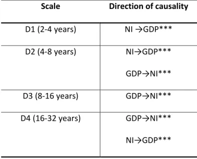
conventional significance levels. The results are found in Table 3.

For the finest scale we find that investment Granger causes growth. On

scale 2, corresponding to dynamics with a period of 4 to 8 years (roughly

business-cycle dynamics), we find that GDP Granger causes investments, and

investments Granger cause GDP (at a significance level of 5 %). The

interdependency of GDP and investments seems reasonable for these short-run

variations since investments directly boost GDP via increased spending and

high GDP growth facilitates investments in infrastructure via government

budget surpluses. On scale 3 we have a clear unidirectional causality from GDP

to investments. Hence, we see that the causality is reversed between scale 1 and

scale 3. In contrast, we have a feedback mechanism between growth and

investments for the coarsest time scale. Hence, the causality relationship

between growth and transport investments is not straightforward, but dependent

on the time scale we analyze. Only time scale decomposition can shed light on

the reversal of causality between growth and investments comparing scale 1

and scale 3. Granger causality tests on raw data indicate a feedback

our results might provide an explanation for the contradicting results of

previous studies. The results of the Granger causality tests should be

interpreted carefully, however, since the choice of lags might affect the results.

It is therefore necessary to conduct additional analyses and comparisons.

Table 3: Granger causality net infrastructure investments (NI) and GDP Scale Direction of causality

D1 (2-4 years) NI →GDP*** D2 (4-8 years) NI→GDP*** GDP→NI*** D3 (8-16 years) GDP→NI*** D4 (16-32 years) GDP→NI*** NI→GDP*** Significance levels: *:1% **:5% ***:10%

In order to investigate the direction of causality we compute the impulse

response functions (IRF) for scale 3, so that we can determine whether higher

growth increase or decreases future infrastructure investment activity on a

longer time scale. An impulse response function traces the response of the

endogenous variables in the system to a shock in one variable. In order to

compute the impulse response function we need to impose some structure on

the system since it is over identified otherwise. The so called Choleski

decomposition provides a minimal set of assumptions for this purpose (Engels,

is arbitrary; in a bivariate VAR there are two different possibilities. In Figure 5

we therefore display the two different possibilities when tracing the cumulative

effect of a GDP-shock. In this case, we can see that the response of

infrastructure investments to a shock in GDP is qualitatively the same in both

cases. The decaying effect is a result of a stationarity of the decomposed time

series.

Figure 4: The cumulative IRF for a shock in GDP on infrastructure investments

Since the data on capital depreciation (consumption of fixed assets) in the

transport and communication sector might be flawed as it possibly does not

reflect true depreciation, we also look at gross infrastructure investments in the

transport and communication sector (see Table 4).

Table 4: Granger causality gross infrastructure investments (I) and GDP Scale Direction of causality

D1 (2-4 years) I → GDP* −.02 0 .02 .04 0 5 10 0 5 10

95% CI cumulative orthogonalized irf step

D2 (4-8 years) I→GDP* GDP→I** D3 (8-16 years) GDP→I** D4 (16-32 years) GDP→I***

Significance levels: *:1% **:5% ***:10%

We see that the Granger causality direction from GDP to investments is even

more pronounced, except for the finest time scale. This indicates that

reinvestments in infrastructure are caused by economic growth and not vice

versa.

A comparison between net infrastructure investments and total net

investments might be elucidative to enable conclusions to be drawn about the

mechanism behind infrastructure planning; that is, if there are any differences

between the decision processes of infrastructure investments and other

investments in the economy. Our results from the Granger causality test for

total investments are provided in Table 4.

For total net investments we have a clear unidirectional causality from net

investments to GDP. This is in contrast to some other studies which have

confirmed that this causal relationship is from GDP to investments. However,

for short-term fluctuations captured by scale 1, we find weak evidence of GDP

causing investments, but stronger evidence of investments causing GDP, that

is, a feedback mechanism. Once again, time-scale decomposition seems to

provide a clearer picture of the relationship due to the fact that the simultaneity

A bivariate VAR might be an over-simplification of reality, since GDP consists

of many other variables that could be covariates to both infrastructure

investments and GDP. We therefore also test for causality in a VAR-model

including private consumption. Still, the qualitative results with regard to the

causality relationship are unchanged (the results are not shown here, but are

available from the author on request).

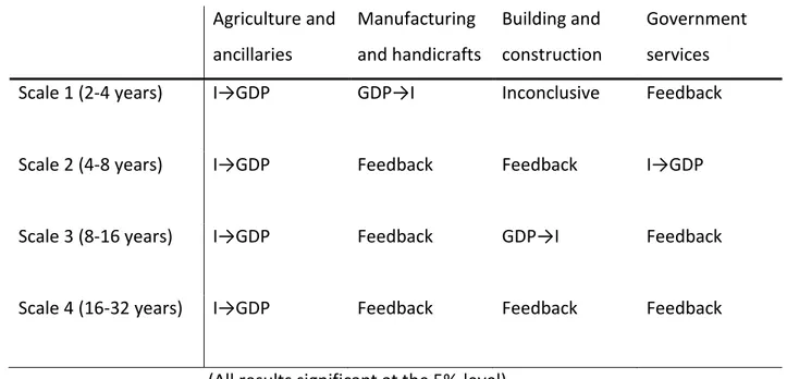
Last but not least, we analyze the causal relationship between

GDP-growth and gross investments in other major sectors of the economy (see Table

6). The pattern revealed for infrastructure investments seems to be unique, but

no clear pattern is detectable for sector-specific investments and growth. For

example, high growth levels in agricultural investments precede high

GDP-growth across all time scales. In comparison, investments in manufacturing,

government services and building/construction are most often characterized by

a feedback-mechanism between investments and GDP. Only investments in the

building and construction sector resemble the unidirectional causality seen for

infrastructure investments for scale 3.

Scale Direction of causality D1 (2-4 years) NItotal→GDP** GDP→ NItotal * D2 (4-8 years) NItotal →GDP** D3 (8-16 years) NItotal →GDP*** D4 (16-32 years) NItotal →GDP*** Significance levels: *:1% **:5% ***:10%

Table 6: Granger causality tests for gross investments (I) in other sectors and GDP Agriculture and ancillaries Manufacturing and handicrafts Building and construction Government services Scale 1 (2-4 years) I→GDP GDP→I Inconclusive Feedback

Scale 2 (4-8 years) I→GDP Feedback Feedback I→GDP

Scale 3 (8-16 years) I→GDP Feedback GDP→I Feedback

Scale 4 (16-32 years) I→GDP Feedback Feedback Feedback

(All results significant at the 5%-level)

4 Conclusions

This paper applies a wavelet-based approach to investigate the relationship

between infrastructure investments and economic activity for different time

scales. We utilize new data on GDP and investments in the transport and

communication sector for the period 1800-2000. Through a scale by scale

decomposition we try to shed light on the scaling properties of causality in the

relationship between infrastructure investments and GDP growth rates.

The findings in this paper indicate that there are considerable correlations

between economic fluctuations and investments and that infrastructure

investments Granger causes growth in the short run and that the reverse is true

for longer-time horizons. This implies that the infrastructure investment

planning process is reactive and not proactive. Considering the risk structure,

positively correlated with overall economic activity; that is, the benefits from

these projects for society as a whole are largest in good times but provide no

insurance during bad times. According to the Capital Asset Pricing Model, the

total risk of an investment is not relevant for estimating the risk of an asset; the

relevant risk measure is the correlation between the payoffs from holding the

asset and the total market performance. The implication for infrastructure

investments is that they are high risk projects for society since the demand for

infrastructure services is positively correlated with economic activity. In

addition, an ex-ante estimation of infrastructure service demand may be highly

uncertain, raising the hurdle rate for these investments and thus, according to

real option theory, leading to a postponement of investments. Other

explanations might be the long planning process for infrastructure projects and

the capacity of infrastructure networks to handle a larger quantity than the

References

Aschauer, D., (1989), Is Public Expenditure Really Productive?, Journal of

Monetary Economics, 23, 177-200.

Edvinson, R., (2005) Growth, Accumulation, Crisis: With New Macroeconomic

Data for Sweden 1800-2000, Almqvist & Wiksell International, Stockholm.

Gallegati, Marco and Gallegati Mauro, (2007), Wavelet Variance Analysis of

Output in G-7 Countries, Studies in Nonlinear Dynamics and Econometrics,

11(3).

Gencay, R., Selcuk, F. and Whitcher B., (2002), An Introduction to Wavelets

and Other Filtering Methods in Finance and Economics, San Diego Academic

Press.

Gramlich, E. M., (1994), Journal of Economic Literature XXXII, 1176-1196.

Granger, C. W. J., (1969), Investigating causal relations by economic models

and cross-spectral method, Econometrica, 37, 24–36.

Granger, C. W. J. and Newbold, P., (1986), Forecasting Economic Time Series,

Johansson, Ö., (1967): The gross domestic product of Sweden and its

composition 1861-1955. Almqvist & Wiksell, Stockholm.

Lindahl, E., Dahlgren, E., and Kock, K., (1937), National Income of Sweden

1861-1930, part one and two. PS King & Son and Nordstedt & Söner.

Lindahl, O., (1956), The gross domestic product of Sweden 1861-1951,

Meddelande från Konjunkturinstitutet, Serie B:20, Konjunkturinstitutet;

Stockholm.

Luoto, J. 2011. Aggregate Infrastructure Capital Stock and Long-Run Growth:

Evidence from Finnish Data. Journal of Development Economics 94, 181-191.

Mokhtarian, P. L., Salomon, I., (2002), Emerging Travel Patterns: Do

Telecommunications Make a Difference?, in: H.S. Mahmassani (ed.),

Perpetual Motion: Travel Behavior Research Opportunities and Application Challenges, Elsevier Science Ltd.

Munell, A. H., (1992), Policy Watch, Infrastructure and Economic Growth,

Journal of Economic Perspectives, 6(4), 189-198.

Thomas, D. S., (1941), Social and Economic Aspects of Swedish Population

Walden T. A. and Percival P. D., (2000), Wavelet Methods for Times Series