Institutionen för Matematik och Fysik
Code: MdH.IMa.Mat.0076 (2006) 10p-AF
MASTER THESIS IN MATHEMATICS /APPLIED
MATHEMATICS
A Java applet for simulation of economy with
Borrowers under costly defaults
by
Basil Wakid Hassan
Magisterarbete i matematik / tillämpad matematik
DEPARTMENT OF MATHEMATICS AND PHYSICS
MÄLARDALEN UNIVERSITYDEPARTEMENT OF MATHEMATICS AND PHYSICS
___________________________________________________________________________
Master thesis in mathematics / applied mathematics
Date:
2007-01-23
Projectname:
A Java applet for simulation of economy with borrowers under costly defaults
Author:
Basi Wakid Hassan
Supervisor:
Dr. Anatoliy Malyarenko
Examiner:
Prof. Dmitrii Silvestrov
Comprising:
10 points
---
Dedicated with love
To my wife Hanan, my son Mustafa,
My daughters Saba and Yasmin,
And to the memory of my father,
My mother
Abstract
This master thesis focuses on the simulation of economy with
borrow-ers under costly defaults. The asset-value dynamics in our model
exhib-its stochastic mean and volatility. A Java program is developed as a
tool for calculation.
Acknowledgements
This study has drawn on the aptitudes, advice and encouragement of
more people that I can possibly acknowledge. I would, however, like to
recognize the contributions of many who have helped.
First, I want to thank my wife, for her support, interest, encouragement,
and children who also have experienced the hefty time demands of this
project and have understood and helped me in numerous ways.
I greatly appreciate the assistance of my supervisor Dr. Malyarenko
Anatoliy who was the major developer of the study guide and
contrib-uted greatly to this project.
I want to thank Prof. Silvestrov Dmitrii, for his role played by
exam-iner this study and appreciate for his efforts and encouragements.
I am very grateful to all my teachers, and other colleagues and
adminis-trative staff of Malardalen University, particularly grateful to
depart-ment of Mathematics and physics for their kind help.
Table of Content
Table of Content...5
1.
Introduction ... 8
1.1. Background ... 8
1.2. Objective ... 9
2.
Mathematical &Background Reviewing of Basak-Shapiro Credit Risk
model ... 10
2.1. Basak-Shapiro Model of the debt contract and default cost... 11
2.2. Basak-Shapiro Optimization problem when debt maturity coincides with Planning horizon(T =T′) ... 12
2.3. Reviewing Mathematical and Background of The study to get the solution ... 14
3.
Analysis and Inferences... 18
3.1. Effect of model parameters on optimal wealth ... 18
3.1.1. Effect of Increase Model Parameters values ... 19
3.1.2. Effect of Wealth relative Frequency Histogram ... 23
3.1.3. Effect of Investment Policy... 24
3.2. Sensitivity analysis of risk exposure function to change in model’s parameters... 27
3.2.1. Effect of debt-contract parameter’s on risk exposure function ... 28
3.2.2. Effect of default-costs parameter’ on risk exposure function ... 31
4.
Java Applet for Basak-Shapiro model... 35
4.1. Introduction ... 35
4.2. Applet: User Guide and Parameters ... 36
4.2.1. J Pane... 36
4.2.1.1. Input panel ... 37
4.2.1.2. Control panel ... 38
4.2.1.3. Output panel ... 38
4.2.2. Debt function trajectory ... 39
4.2.3. Wealth function ... 40
4.2.4. Risk investment function... 40
4.2.5. Numerical results... 41
4.2.6. Default Relative Frequency Histogram... 41
4.2.7. Wealth Relative Frequency Histogram ... 42
4.2.8. Joint Histogram ... 42
4.2.9. Final Numerical Results ... 43
4.2.10. Risk Exposure function ... 44
5.
Conclusion ... 45
6.
References ... 47
List of Figures
Figure 1 Debt value function with defaults region boundaries ... 13
Figure 2 wealth function ... 18
Figure 3 debt value function... 18
Figure 4 wealth function when (F) increase... 19
Figure 5 debt value function when(F) increase ... 19
Figure 6 wealth function when(β) increased ... 20
Figure 7 debt value function when(β) increased ... 20
Figure 8 Wealth function when(β) reach to limit of one... 20
Figure 9 debt value function when(β) reach to limit of one... 21
Figure 10 Wealth function when
( )
λ increased... 21Figure 11 debt value function when
( )
λ increased... 22Figure 12 Wealth function when
( )
φ increased ... 22Figure 13 debt value functions when
( )
φ increased... 22Figure 14 wealth histogram when (F) is very small... 23
Figure 15 wealth histogram... 24
Figure 16 risky investment function for simulated trajectories that lead to no default positions ... 25
Figure 17 risk exposure function for simulated trajectories that lead to no default positions ... 25
Figure 18 debt value function for simulated trajectories that lead to no default positions ... 26
Figure 19 Java applet viewer: Risk exposure function ... 27
Figure 20 for F = 2 ... 28 Figure 21 for β = 0.6... 29 Figure 22 for F = 0.7 ... 30 Figure 23 for β = 0.4... 30 Figure 24 for φ = 0.5 ... 32 Figure 25 for λ = 0.9... 32 Figure 26 for φ= 0.015 ... 33 Figure 27 forλ = 0.01... 34
Figure 28 Java Applet Viewer: BasakShapiro2 credit risk model ... 36
Figure 29 error messages for retaining rate value ... 37
Figure 30 control panel ... 38
Figure 31 output panels ... 38
Figure 32 output panels ... 39
Figure 33 debt value functions ... 39
Figure 34 wealth function ... 40
Figur 35 risk investment policy... 40
Figure 36 numerical results ... 41
Figur 37 default relative frequency histogram ... 41
Figure 38 wealth relative frequency histogram... 42
Figure 39 joint histogram ... 42
List of tables
Table 1 for F = 2... 28 Table 2 for β = 0.6... 29 Table 3 for F = 0.7... 30 Table 4 for β = 0.4... 31 Table 5 for φ = 0.5... 32 Table 6 for λ = 0.9 ... 33 Table 7 forφ= 0.015... 34 Table 8 for λ = 0.01 ... 341. Introduction
1.1. Background
Risk managers are responsible to monitored risk carefully due to their damage affects on busi-nesses. They should be able to identify various risk exposure, measured and controlled.
Generally, risk defined as volatility of unexpected outputs. Firm face various types of risk such as business and no business risk. The most interest risk is, in this study, financial risk, specifi-cally credit risk. These risks focus on potential losses in financial market due to fluctuations in interest rate or defaults on financial commitments.
Commonly, risk manager’s aims to measure sources of risk, as precisely as possible, purpose to controlling and suitably price risks. So that risk regard as the magnitude of possible loss or volatility, as measured by standard deviation of the possible income or revenue of portfolio (investment or trading) over specific horizon [1].
Financial risks can be classified broadly by several categories such as, market risks, credit risks, liquidity risks, operational risks and legal risk.
The source of risks can be mainly comes from two factors:
Default risk, is define as the objective assessment of default probability for the counterparty combined with the loss given default.
Market risk or credit exposure, is defined as the probable future loss that may be happened due to a decrease in market value. Generally this occurs because the observed market rates subject to changes – e.g. yield curves, implied volatilities, and spot exchange rates.
The quantification of credit risk recently gains great attentions and become a large subject area. Increasing borrowing transactions specifically through private sector in recent years and option to default, as increased default probability of debt contracts, led to raise the need for the credit risk models whose estimate the dynamic of the borrower asset value and credit risk as part of their debt.
Often, default occurs at maturity and when the asset value of borrower less than the face value of a debt contract. Because the dynamic of asset price managed by the borrower so the prob-ability of a credit risk arise.
Credit risk defined as financial loss due to borrowers may be unwilling or unable to fulfill their contractual obligations. This loss encompasses exposure or amount at risk, represented here by the face value of the instrument or debt. And retaining rate represents the fraction recovered given default, or one minus the loss given default [2].
Basak-Shapiro models take a zero-coupon debt contract as borrowers leverage instrument that may default occur upon maturity date.
This study considers only the state where the date of repay the debt is coincides with borrowers planning horizon.
Borrowers optimal terminal net worth and debt value function and the others functions are bounded in three state of the economy area: no default, default and between as resistance of default. The models illustrate a different economics behavior of borrower optimal wealth func-tion across the above regions. Costs of default affect the optimal policy of the borrower with different manner through the horizon of default region.
1.2. Objective
Our objective is to use Basak-Shapiro model, as abase of this study, for the purpose of model-ing debt contract and costs of default that affects optimal policies of the borrower and analysis the associated investment and consumption policies.
Principally, the aim of this study is to creating an applet by trying to write a program in Java language. This program will truly enable end user dealing easily with numerical and graphical outputs of this model. To achieve this goal the study will adopt different methods than were used in Basak-Shapiro model for estimation formulas and depicting the figures.
So that, the study intending to design and realizes an applet layout that best display the above mentioned requirements used specially for this model. Our goal also to make this program capable to meet the end user needs and provide a wide flexibility in sensitivity analysis plus performing the necessary calculation for a decision making.
For accomplish these objectives, the study will figure out the appropriate codes and mathemat-ics and write a program in Java language that display an applet with a number of panels, but-tons, labels, progress bar, field among others, suitable for this model.
2. Mathematical &Background Reviewing of
Basak-Shapiro Credit Risk model
The purpose of this section is to describe and reviewing Basak-Shapiro models which used as background of this study and facilitate the following of this model [3].
The financial market in this model is a finite –horizon, [0-T ‘] which containing a single con-sumption good.
The model defines the uncertainty by filtration process of the probability space
which has also an N-dimensional Brownian motion representing by the following [4]:
[
Ω,F,{Ft},P]
]. , 0 [ , )] ( ..., ),... ( [ ) (t w1 t w t t Tw = N T ∈ ′ The stochastic processes in this model are adapted to }
{F , wheret The financial market containing N+1 investment instrument one instan-taneously risk-free and the others are risky. The dynamics of the investment net return have the following vector: ] , 0 [ T t∈ ′ , (1) ⎟⎟ ⎟ ⎟ ⎠ ⎞ ⎜⎜ ⎜ ⎜ ⎝ ⎛ + dt t r t dw t dt t ) ( ) ( ) ( ) ( σ μ r = interest rate μ= drift coefficients
(
)
T Nμ
μ
,..., , with the volatility matrix σ ≡{
σij,i=1,...,N;j=1,...,N}
which might be path dependent.If the market is complete and free of arbitrage it will exists unique state price density process
( )
ζ which have the following differential equation:dζ(t)=−ζ(t)
[
r(t)dt+Κ(t)Tdw(t)]
, ………… (2) ζ(0)=1.In the equation (2) Κ(t) representing the market price of risk and equal to
[
t r t I]
t
t) ( ) ( ) ( ) ( ≡σ −1 μ −
κ , and I ≡(1,...,1)T.
The Arrow-Debreu price is measured by ζ(T ′,ω)per each unit of probability and consumption good taken in the stat ω∈Ω at timeT ′ .
A zero-coupon bond which matures at date T [5] is a contract that guarantees the holder to re-ceive one Unit of money (dollar, kronor, sterling …..) at the date T. The borrower in this model is restrict by this instrument to get the initial wealth of W(0), which is equal to the net of bor-rowing proceeds that the borrower will get it at the time = 0.
At the end of the nonnegative planning-horizon wealth the borrower will receive a terminal net worth W (T '). The borrower chose to invest the borrowing proceed in an investment policy (θ) Symbolize the vector of fractions of wealth that the borrower intends to invest it in each risky investment opportunity. The wealth process W (t) before the
debt-maturity date satisfies the following equation
[
T N t t),... ( ) ( 1 θ θ ≡]
) ( ) ( [ ) ( ) ( ){ ( ) (t W t r t t t r t dW = +θ T μ − 1]}dt+W(t)θ(t)Tσ(t)dW(t). (3)The known value is interpreted as the initial wealth while the value represents the terminal net worth. Before debt-maturity the total value of the assets , managed by bor-rower, is ) 0 ( W W(T′) ) (t V V(t)=W(t)+D(t). Where equal the value of the debt. D(t)
The objective function which represents the expected value that the borrowers wish to maximize is assumed twice continuously differentiable severely concave, severely increasing
with , and . )] ( [W T v ′ ∞ = ′ → ) (
lim
0 x v x 0 ) (lim
′ = ∞ → x v x2.1. Basak-Shapiro Model of the debt contract and default
cost
The main goal of Basak-Shapiro models is to verify if the default costs (when it occurs) have an affect on the optimal policies of the borrower. The default able debt contract has two charac-teristics:
First, when the default occurs, the lender can calculate only a fraction of the borrower’s assets which is reproduced in variation from the absolute priority rule.
Second, the declaration of the default is happened in spite of that the borrower have enough assets to service the debt. The debt contract between borrower and lender has the following Structure:
Assumption1. The payoff of a zero-coupon debt contract is
D(T)=min{(1−β)V(T),F}.
F Is the face value of the debt contract and maturity date isT ≤T′, β representing the retain-ing rate and equal to0≤β ≤1 .
When the borrower is enabling to fully repay the face value at debt-maturity dateT ≤T′, the default occurs. In this case the debt value will be equal to: D(T)=(1−β)V(T)<F,and the
default boundary will be equal to
) 1 ( β β − F
and this is involving that the borrower’s solvency should be ) 1 ( ) ( β β − ≥ F T
W . Where βν(t) represent the value that the borrower keeps hold of it Upon default .The borrowers assets divide into two parts, tangible part of asset,(1−β)V(T) which guarantee the repaying of the debt when it is liquidizes, and the intangible part
) (T
βν such as human resources and administration and organizational skills and knowledge’s. Since the claim’s covered by tangible assets upon default the borrower then can be able to use the intangible assets to generate future cash flows. The debt maturity date (T) is fixed ahead so the default perhaps take place only in this deterministic date, or coincide with planning horizon date . (T ′)
Assumption2. At maturity date T, and upon the default occur, the borrower incurs the
follow-ing defaults costs
⎩ ⎨ ⎧ = < − + Φ = . ) ( , 0 , ) ( )], ( [ ) ( F T D F T D T D F T C λ
As it stated before the default happened when [D(T)<F],so Φ≥0 represent the fixed cost of the default that the borrower incurs andλ≥0equal to the proportional costs with the above
total cost of default .Default cost may be interpreted as direct or in-direct cost because both cost component may include these expenses.
) (T
C
)] (
[F −D T Equal the amount of default and λrepresent the proportional cost per unit of default so the total variable costs will be the multi-plication result.
In case we don’t have a debt, the investor depend on the self financing, the benchmark invest-ment model (hence-forth B) will be used for comparison. The optimal solution of this model is B-model with F=0 and (V=W). WB(T′)
2.2. Basak-Shapiro Optimization problem when debt
matur-ity coincides with Planning horizon
(T =T′)The model gives us a solution of the optimization problem of the borrower which is limited by the coincidences of the two dates, debt contract maturity and planning horizon date(T =T′). According to default cost, it is quit possible that the borrower declare his or her default ness at time T. The solution gets the following characteristics:
A. The optimization problem is stated as following:
Try to find
max [ ( ( ))].
)
(T E W T
W ν
Subject to the constraint
E{ζ(T)[W(T)+C(T)]}≤W(0). (4) The borrower s budget constraint shows that the initial wealth W (0), resulted from the pro-ceeds of net borrowing process, must be enough to cover time T values (terminal wealth plus probable costs).
In what follows we suppose that(T =T′),ν(W)=W , r(t)=r and k(t) = k.
Basak and Shapiro propose the following proposition to find the optimal solution:
When debt maturity date agree with the borrower’s planning horizon(T =T′), the optimal so-lution of the borrower’s optimal net worth will be
W*(t) = ⎪ ⎪ ⎪ ⎩ ⎪ ⎪ ⎪ ⎨ ⎧ ≤ − − − < ≤ − < default T if T y I ce resis default T if F nodefault T if T y I : ) ( )] ( ) 1 ( [ tan : ) ( 1 , : ) ( )] ( [ * * * * * ζ ζ ζ β λ β β ζ ζ ζ β βζ ζ ζ (5)
Where I (.) is the inverse function ofν′(.),ζ* ≡ν′
[
βF/(1−β)]
/y and solve the following system: 0 , * * ≥ ≥ y ζ ζ[
( )]
−[
( )]
=[
( )− ( *)+Φ]
* * * * ν ζ ζ ζ ζ ζ ν I x I y x I y I ywithx≡βy/
[
β +λ(1−β)]
,E{ζ(T)[
W*(T;t)+C(W*(T;t))]
}=W(0). And the benchmark bor-rower’s optimal terminal net worth is WB(T)=I[
yBζ(T)]
, wheresolves . B y ) 0 ( ))} ( ( ) ( { T I yB T WB E ζ ζ =
And they depict the borrower’s time-T optimal wealth with relation to the time-T B-policy, at time , with respect to the price of the consumption good
) ( * T W ) (T =T′ ζ(T)as independent
variable. They found that the borrower show three separate prototypes of economic behavior which can be charted into three regions of the states space:
A. No default
B. Default resistance. The optimal wealth is constant and does not change by increasing the price ofζ(T) .
C. Default.
Interval[0,ζ*)represents no default region, the good state, where ζ* coming just after the ter-minated of no default region. Sinceζ(T)<ζ*the borrower fulfils all his obligations toward the
lender and don’t defaulting. The intermediate interval the area in which the borrower resist to announce default ness and called default resistance region or
(resis-tance).While the Interval consists of default region, the bad states, in which the bor-rowers no more can keep his financial obligations toward the lender.
) ) ( [ζ* ≤ Tζ <ζ* ) ( [ζ* ≤ζ T
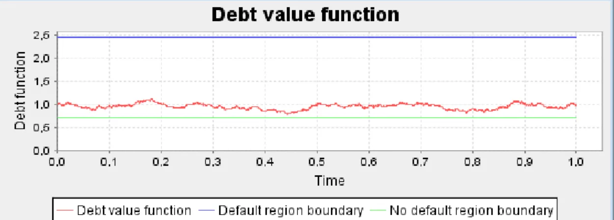
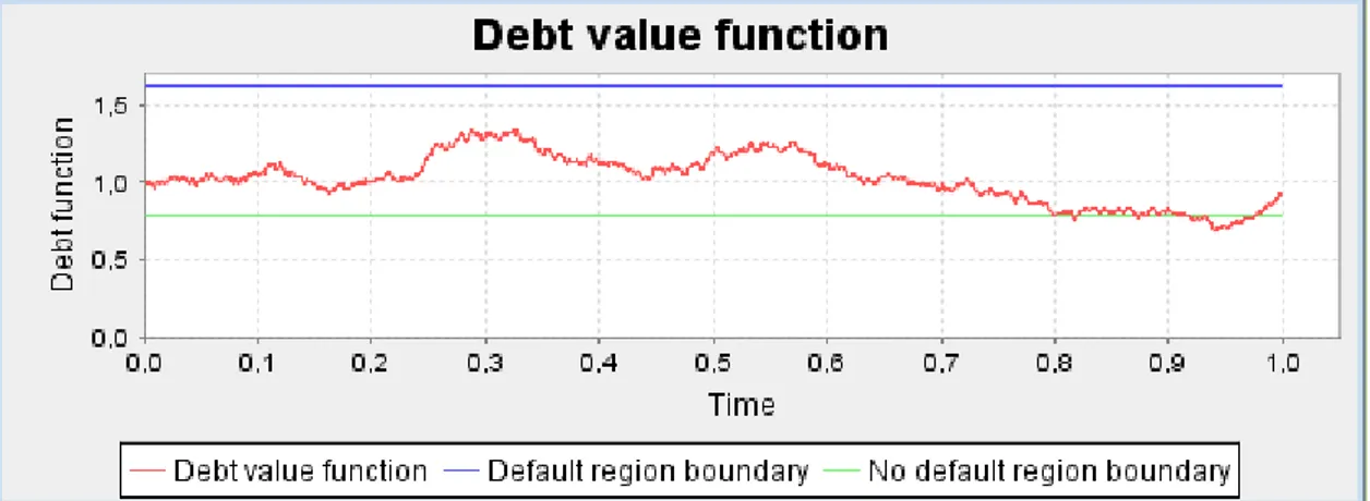
The resistance region, between the two lines, as shown in figure 1 below emerge due to unde-sirability of costly default as we can consider it as financial distress costs that is leading to obliterate the business and loss the resources.
The minimum level of the optimal wealth should be kept by the borrowers as a buffer against the default is correspond to the value of the default boundary,
β β − > 1 ) ( * F T
W , and this indicator
will be used to conclude the default state from the estimated data in this study.
Figure 1 Debt value function with defaults region boundaries
2.3. Reviewing Mathematical and Background of The study
to get the solution
We start by introducing an auxiliary variable as the solution to the following equation and take into consideration that
* ζ y z= 1 = γ : ) 1 ( ln 1 )] 1 ( )[ 1 ( )] 1 ( [ ) ( ln * * β β β λ β β ζ β β β ζ β β λ β − + = − + − − Φ − + ⎥ ⎦ ⎤ ⎢ ⎣ ⎡ + − F y F y ) 1 ( ln 1 )] 1 ( )[ 1 ( )] 1 ( [ ) ( ln β β β λ β β β β β β β λ β − + = − + − − Φ − + ⎥ ⎦ ⎤ ⎢ ⎣ ⎡ + − F z F z ) 1 ln( ln 1 )] 1 ( )[ 1 ( )] 1 ( [ ln ) 1 ( ln( β β β λ β β β β β β β λ β = + − − − + − − Φ − + − − + z F z F ) 1 ln( ln 1 )] 1 ( )[ 1 ( )] 1 ( [ ln ln ) 1 ( ln( β β β λ β β β β β β β λ β = + − − − + − − Φ − + − − − + z F z F ) 1 ( ln( ) 1 ln( ln ln 1 )] 1 ( )[ 1 ( )] 1 ( [ ln β β β β λ β β λ β β β β β = + + − − − + − − + − − Φ − + − z F z F ) 1 ( ln( ) 1 ( ln 1 )] 1 ( )[ 1 ( )] 1 ( [ ln 2 β λ β β β β λ β β β β β − + − ⎟⎟ ⎠ ⎞ ⎜⎜ ⎝ ⎛ − + = − + − − Φ − + − z F z F ⎟⎟ ⎠ ⎞ ⎜⎜ ⎝ ⎛ − + − + = − + − − Φ − + − ) 1 ( )( 1 ( ln 1 )] 1 ( )[ 1 ( )] 1 ( [ ln 2 β λ β β β β λ β β β β βF z F z ⎟⎟ ⎠ ⎞ ⎜⎜ ⎝ ⎛ − + − + = − − + − − Φ − ) 1 ( )( 1 ( ln 1 ln )] 1 ( )[ 1 ( )] 1 ( [ 2 β λ β β β β λ β β β β β F z z F (6)
In Basak and Shapiro model’s they propose isoelastic objective function that is equal to , 0 ), 1 /( ) ( = 1− −γ γ > ν γ where W
W conditioned by state prices are lognormal distributed and associated with constant interest rate and risk market price. Under these conditions they derived an explicit direct expression to calculate the borrower’s optimal wealth and investment policy prior the debt maturity and planning horizon as stated below:
[
]
[
]
⎪ ⎪ ⎪ ⎩ ⎪⎪ ⎪ ⎨ ⎧ − ⎪ ⎪ ⎭ ⎪ ⎪ ⎬ ⎫ ⎥ ⎥ ⎦ ⎤ ⎢ ⎢ ⎣ ⎡ − − − − − + ⎥ ⎥ ⎦ ⎤ ⎢ ⎢ ⎣ ⎡ − = − − γ γ ζ ζ ζ β β ζ 1 * 1 * 2 ) ( 1 * ) ( ) ) ( ) ( 1 ) ( ) ( ) ( t y d N t T X d N e F t y t T X t W rT t[
]
[
]
[
]
{
}
(1 ) ) 1 ( / ) ( ) ( ) ( ) ( 1 1 * 1 * 2 ) ( β λ β β β λ β ζ β ζ ζ β β γ + − ⎪⎩ ⎪ ⎨ ⎧ ⎪⎭ ⎪ ⎬ ⎫ − + − − − − ⎟⎟ ⎠ ⎞ ⎜⎜ ⎝ ⎛ Φ − − − − t y d N t T X d N e F rT t (7)Here we have t<T, N (.) represents the standard-normal cumulative distribution function. Where s k r s x ⎥ ⎥ ⎦ ⎤ ⎢ ⎢ ⎣ ⎡ + − ≡ γ γ γ 2 ) 1 ( ) ( ln 2 And when γ =1 So, Ln x(s) = 0 X(s) = 1 X (T-t) = 1 And
[
]
( ) ( ) 1 ) ( ) ( * 1 t z t y t y t T X ζ ζ ζ ζ γ = = − (8) And z = yζ*.Next, introduce two auxiliary functions:
t T k t T k r t x x d − − − + = ln( / ( ) ( /2)( ) ) ( 2 2 ζ d1(x)=d2(x)+ k T −t , 1 1 * γ β β ζ ⎥ ⎦ ⎤ ⎢ ⎣ ⎡ − ⎟⎟ ⎠ ⎞ ⎜⎜ ⎝ ⎛ = F y y and solve * ζ
[
]
[
]
γ γ γ β β γ β λ β β ζ β β β ζ β β λ β γ γ − − ⎟⎟ ⎠ ⎞ ⎜⎜ ⎝ ⎛ − − = − + − − Φ − + ⎥ ⎦ ⎤ ⎢ ⎣ ⎡ + − − 1 * / ) 1 ( * 1 ) 1 ( 1 ) 1 ( ) 1 ( ) 1 ( ) 1 ( ) 1 ( F y F y AndW*(0,y)=W(0). Where * * ) 1 ( ζ β β ζ zF − = .[
]
( ( )) ) ( ) ( ( 1 ) ( ) ( 1 * * 2 ) ( * * ζ ζ ζ ζ β β ζ ζ d N t z x d N e F t z t W rT t − − − − + = − −[
( )]
) 1 ( 1 * 2 ) ( ζ β λ β β β β d N e F rT t − − + ⎟⎟ ⎠ ⎞ ⎜⎜ ⎝ ⎛ −Φ − − − −[
( )]
) 1 ( * ) 1 ( ) ( ) ( * 1 1 β λ β ζ β β λ β ζ β γ d N t y t T x − − + ⎥ ⎦ ⎤ ⎢ ⎣ ⎡ − + − +(
)
[
]
[
]
*) 1 1 ( ) 1 ( * ) 1 ( /( )) ( ) ( ζ β λ β β β λ β ζ β γ d N t y t T x − − + − + − +(
)
(
( ))
) ( ) ( 1 ) ( ) ( 1 * * * 2 ) ( * * ζ ζ ζ ζ β β ζ ζ d N t z d N e F t z t W rT t − − − − + = − −(
( ))
) 1 ( 1 * 2 ) ( ζ β λ β β β β d N e F rT t − − + ⎟⎟ ⎠ ⎞ ⎜⎜ ⎝ ⎛ −Φ − − − −(
( ) ) ( * 1 * ζ ζ ζ d N t z − +)
(9) Now, the obvious equality W*(0,y)=W(0) becomes an equation with respect toζ*.Solving this equation, we obtain the values of ζ*andζ*. When t = 0, soζ(t)=ζ(0)=1.
AndW*(0)= W(0)=1.
Then the auxiliary functions are:
T k T k r x x d ( ) ln( ) ( /2) 2 2 − + = . T k x d x d1( )= 2( )+ .
From equation (9) we get, when t = 0, then the following:
[
( )]
( ( )) 1 ) 0 ( 1 * * * 2 * * ζ ζ ζ β β ζ d N z d N e F z W rT − − − − + = −(
( ))
) 1 ( 1 * 2 ζ β λ β β β β d N e F rT − − + ⎟⎟ ⎠ ⎞ ⎜⎜ ⎝ ⎛ −Φ − − −(
) ( * 1 * ζ ζ d N z − +)
= 1 (10)Simplifying equation (10) we get: ⎟⎟ ⎠ ⎞ ⎜⎜ ⎝ ⎛ − − − ⎥ ⎦ ⎤ ⎢ ⎣ ⎡ ⎟⎟ ⎠ ⎞ ⎜⎜ ⎝ ⎛ − − − + = − * 1 * * 2 * * 1 ( 1 1 ) 0 ( ζ β β ζ ζ β β β β ζ zF d N z zF d N e F z W rT
(
( ))
) 1 ( 1 * 2 ζ β λ β β β β d N e F rT − − + ⎟⎟ ⎠ ⎞ ⎜⎜ ⎝ ⎛ Φ − − − −(
) ( * 1 * ζ ζ d N z − +)
= 1 (11)In the equation (11) the only unknown is . So we found an explicit direct expression to solve the equation for and use this value to get the value of equation (10) as mentioned before.
*
ζ
*
ζ
The fraction of wealth invested in the risky investment opportunities is:
θ
*(t)=m*(t)θ
B(t), (12) Where B = 1[
σ(t)T]
−1k
, γθ
which is equal to[
( )T]
1k
, B t − = σθ
(13) The following equation calculates the risk exposure of the borrower:(
)
(
)
⎢ ⎣ ⎡ − − + ⎟⎟ ⎠ ⎞ ⎜⎜ ⎝ ⎛ − − − − − − = − − ( ) ) 1 ( 1 ) ( 1 ) ( 1 ) ( * 2 * 2 * ) ( * ζ β λ β β φ β β ζ β β d N F d N F t W e t m t T r(
)
⎥ ⎥ ⎥ ⎦ ⎤ − ⎟⎟ ⎠ ⎞ ⎜⎜ ⎝ ⎛ + − − − − − + − t T d z Fk
) ( ) 1 ( 1 ) 1 ( * 2 ζ ϕ β β λ β φ β β β λ β β . (14)In equation (14) ϕ
( )
⋅ represent the standard-normal probability distribution function.Basak and Shapiro proposed exposure of the risky investment with relation to benchmarks pol-icy is bounded by:
Ifφ =0, then0≤m*(t)≤1 . And ifφ >0, then0≤m*(t)>1
3. Analysis and Inferences
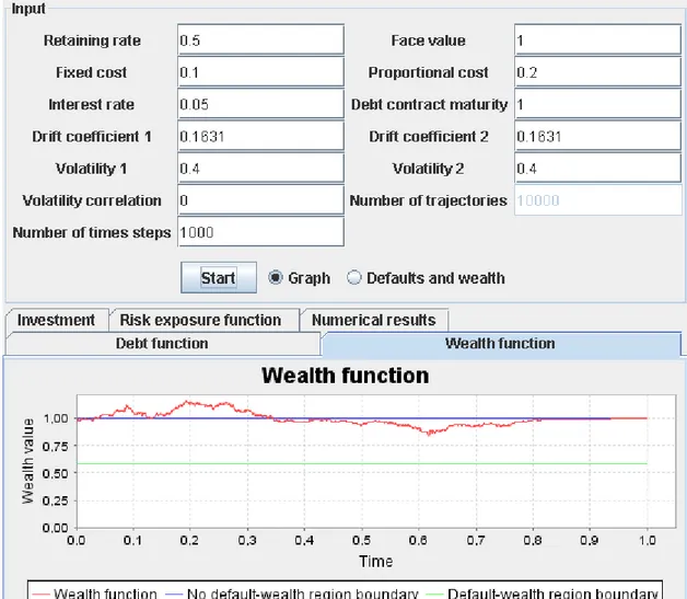
3.1. Effect of model parameters on optimal wealth
Figures 2and 3 below illustrate Java applet viewer for wealth function and debt value function
Figure 2 wealth function
In order to demonstrate the effects of the parameters F,β,λ,φ,on the optimal wealth We shall take the following cases:
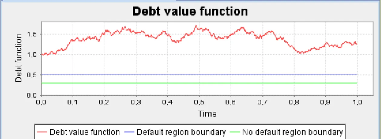
3.1.1. Effect of Increase Model Parameters values
The figure 2 above shows the wealth function with respect to times periods and no de-fault and dede-fault boundaries, and , while figure 3 depict the debt value function with respect to the time periods and region boundaries,
) ( * t W ) ( * * ζ W W*(ζ*) *
ζ and . Parameters used in portray the figures is shown in the input panel. The program gives the user a high flexibility to inspect the dependency of the optimal solution on the parameters
* ζ , , , ,β λ φ
F which it is obvious seen below when we shall try to change the parameters values and demonstrate the results?
As the face value (F) increased from 1 to 2, or the retaining rate
( )
β increased from 0.5 to 0.6. The no default-Wealth and default-Wealth region boundaries, and , increased consequently. But the opposite effect then happened on the no default and default region boundaries, ) ( * * ζ W W*(ζ*) *ζ and , which makes them decrease and led to reduce the size of the resistance region as shown clearly in figures 4 , 5 and 6,7 below :
*
ζ
Figure 4 wealth function when (F) increase
Figure 6 wealth function when (β) increased
Figure 7 debt value function when (β) increased
As the retaining rateβreach to limit of one (as we calculate it here with 0.99999) the no de-fault-wealth region boundary = 99999, and the dede-fault-wealth region boundary = 4077.5. While region boundaries,ζ* andζ*, will be equals to 0.00001 and 0.00006 respectively. Inspecting the figures 8 and 9 below give as an idea about that:
Figure 8 Wealth function when (β) reach to limit of one
Figure 9 debt value function when (β) reach to limit of one
The effect of reaching the retaining rate limits make the optimal wealth value to be very small, around 1.35, and this is indeed explain the reason behind disappearing of wealth func-tion from the Figure 8.In addifunc-tion to that the probability of default, thus, will be (1) that’s mean a surly default and explain also the vanish of the resistance region in Figure 9 which in fact leads to extend the default region over all the sates and incur the maximal cost of default in spite of the value of the debt, D(0), equal to zero.
If we increase the proportional cost parameter,λ,from 0.2 to 1.0 then we succeed to decrease the probability of default from 0.1432 down till 0.0098, in addition getting an increment of the region boundary valueζ*from 1.61 up till 2.45 and lowerζ* from 0.79 down till 0.72, resulting to expand the resistance region in both directions and raise the optimal wealth value from 1.1 to 1.3 and sustain it to be over no default-wealth region boundary which guarantee a good result at the bad states. Figures 10, 11 illustrate the above results.
) (
*
T W
Figure 11 debt value functions when
( )
λ increased
The effect of increasing the fixed costs,φ, from 0.1 to 0.5 reflected directly by extends the re-sistance region from (0.79, 1.61) till (0.71, 4.6) respectively and produce a sharp reduc-tion in the probability of default as it’s reach’s till 0.0001 in addireduc-tion to eliminating the burden of fixed default costs, which is shown in Figures 12 and 13 below:
* *,ζ
ζ
Figure 12 Wealth function when
( )
φ increased
Figure 13 debt value functions when
( )
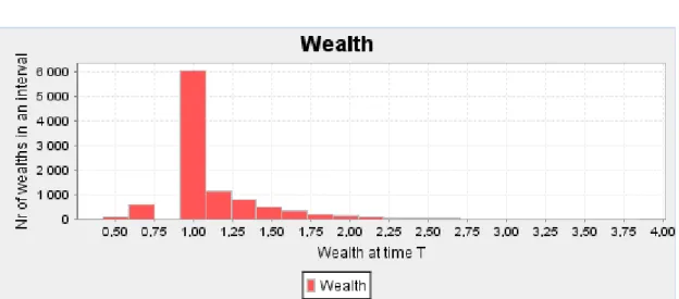
φ increasedThe discontinuity in optimal wealth function disappear when the value of the fixed costs reach to very small amount,0.000001, participated in shrinking of both region boundaries to be(0.89, 1.07) and default boundaries and to be ( 1, 0.9986) as it is shown in Figure 14 clearly . * *,ζ ζ ) ( * * ζ W W*(ζ*)
Figure 14 wealth histograms when (F) is very small
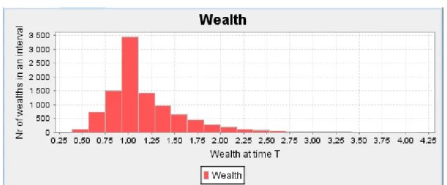
3.1.2. Effect of Wealth relative Frequency Histogram
Let know examine the wealth relative frequency histogram which represent the number of tra-jectories, 10000, simulated to calculate the optimal wealth’s value W*(T)at time T.
A chart is build by subdividing the axis of optimal wealth at time T into intervals of equal width.
Over each interval construct a rectangle, such that the height of the rectangle is relative to the part of the total number of the wealth baths (trajectories) falling in each cell. The relative fre-quencies (fraction of total number of wealth baths), compute for each interval, are shown in Figure 15.
Our objective of depicting the histogram is to make inferences, and the accompanying wealth histograms are sufficient for our objectives.
The probabilistic interpretation that can be derived from the frequency of wealth at time T his-togram is that the likelihood that it will fall in a given interval is proportional to the area under the histogram lying over that interval [6].
Correspondingly the wealth histogram analogous to the shape of the probability density func-tion of the terminal wealth policies that was menfunc-tioned in Basak and Shapiro models.
The area of the high rectangle in the Figure 15 represents a similar proportional expression To the probability mass build up in the optimal wealth at time T. Consequently it is clear that this rectangle constructed at the interval contains the mid point = 1, correspondent to the value of the no default-wealth region boundary
) 1 ( ) ( * * β β ζ − = F
the wealth histogram correspond to discontinuity with no states cover optimal wealth values between ( *) and * ζ W
[
]
⎭ ⎬ ⎫ ⎩ ⎨ ⎧ − + = ) 1 ( ) ( * * * β λ β ζ β ζ y WI
.Viewing Figure 15 shows the rectangles in the no default-wealth region move to the right with decreasing area of these rectangles meaning more wealth with less probability.
Interval that consist of the value of the mean wealth = 1.12223 reflect the heights probability. Whereas intervals hold the default-wealth region = 0.5875 with two rectangles de-creases when moving to the left meaning less wealth with less probability.
) ( *
* ζ
W
Figure 15 wealth histogram
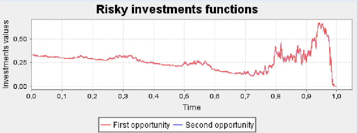
3.1.3. Effect of Investment Policy
Often it is possible to gives a concise and helpful description of a situation by drawing a graph. For example, Figure 16 describes investment values of the fraction of wealth’s invested in each opportunity (here we have first opportunity) at various times up till debt maturity.
The graph shows that the longer the time the more the borrower’s risky investment func-tionsθ*(t).So the fractions of the wealth in risky investment grow larger as time passes. But there is maximum size that value cannot exceed nearby maturity. The maximum size re-flect the restrictions imposed, when default been likely, by the obligations fulfillment of the borrow debt contract at maturity. This enforces the borrowers and discourages him from taking additional risk and the function decay down till almost risk less position.
This policy is adapted when the program simulated trajectories that lead to no default positions and the program can shows also opposite graphs that lead to default positions (of course this is happen when the user tries to simulate several trajectories by pushing the start button) which may gives the user a high flexibility and advantage when he or she working within this pro-gram.
Figure 16 risky investment functions for simulated trajectories that lead to no default positions
In Figure 17 the program have been drawn the graph that depicts the risk exposure func-tionm*(t).
As we can see the function fluctuated through the time. The graph describes a change that is taking place. The amount of money invested in the risky opportunities is changing as time passes. Program provides mathematical tools to study each of these changes in a quantitative way.
From comparing the two Figures 16 and 17 we can illustrates the relationship between the value of amount invested in the risky opportunity and the degree of risk that borrowers encoun-ter. Where amount invested in the risky opportunity proportional with borrowers risk exposure, as the two graphs shows that clearly.
Figure 17 risk exposure function for simulated trajectories that lead to no default positions
Figure 18 debt value functions for simulated trajectories that lead to no default positions
The simulated trajectories that depicts the graphs of the functionsθ*(t),m*(t)andζ(t)reveal the borrowers optimal policy in the times interval [0.0 - 0.8] characterized by a declining of the portion invested in risk opportunity (opportunities) because the borrowers seeking to secure the default-resistance level and guarantee the debt value functionζ(t)left between default bounda-riesζ*(t),ζ*(t)as shown in Figures 16,17and 18 above.
As the time pass, specifically in a time interval [0.8 – 0.95], the borrower’s seek to rise the risk portion of invested wealth and consequently led to grow the borrowers risk exposure.
The need of taking more risk generated from necessitates covering potential default cost as well as default-resistance costs.
Of course anticipating favorable economic conditions induce for more investment in a risky opportunities but this will not continuous until the end.
As time headed for maturity, of the debt contract, nearby and threaten of default is very likely. The borrower prefers risk less investment that may be helps him at least to fulfill his obliga-tions or cover the potential default costs.
3.2. Sensitivity analysis of risk exposure function to change
in model’s parameters
One of unique or distinct feature the program that can provide till users is his ability at conduct the sensitivity analysis among different parameters used in the model and displays the mutual effects and result graphically and numerically.
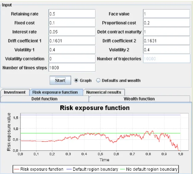
Figure 19 display the parameters used in calculating risk exposure function and the associated graph of this function, for a trajectory have been chose randomly.
Figure 19 Java applet viewer: Risk exposure function
As it mentioned before when debt maturity coincides with borrower’s planning hori-zon
(
T =T′)
.Then values of γ =1andW(0)= k1, =0.4. Then:ζ* =0.79047,ζ* =1.61444 Additionally, effected parameters on the exposure functions can be divided into two types: First: debt-contract parameters(F,β)Second: default-costs parameters(φ,λ)
3.2.1. Effect of debt-contract parameter’s on risk exposure
func-tion
To illustrate the effects of changes in values of(F,β), Figures 20, 21, 22 and 23 and schedules (1, 2, 3, and 4) display the situation when increasing and decreasing the values of by 2 and 0.7 respectively ) (F Figure 20 for F = 2 Table 1 for F = 2
Figure 21 for β = 0.6
Table 2 for β = 0.6
Increasing F form 1 to 2 and βfrom 0.5 to 0.6 correlated with lower in default boundary till in case changing the value of F and
till if changing 51263 . 0 , 29943 . 0 * * = ζ = ζ 86859 . 0 , 50416 . 0 * * = ζ = ζ β.
Subsequently, the probability of default rises sharply and reaches to one. These changes also have an impact on shrinking the resistance region which is displayed in the above Figures and schedules.
Additionally, decrease the value of F till 0.7 andβ till 0.4; generate an opposite effect on the risk exposure function and the above mentioned parameters that participated in build up this function as displayed in Figures 22, 23 and schedules 3 and 4.
Risk exposure function generally become sensitive to the reductions in the values of F andβ. The likelihood of default almost vanish(equal 0.0012 When decreasing F and 0.001 with β de-creasing) which contribute in enhance the financial position’s of the borrower’s by lowering the risk and allowing avoidance of penalties of default through wideness the resistance re-gion.
Figure 22 for F = 0.7 Table 3 for F = 0.7 Figure 23 for β = 0.4
Table 4 for β = 0.4
3.2.2. Effect of default-costs parameter’ on risk exposure
func-tion
The source of risk is not only restricted with debt-contract parameter’s, but it’s expand to com-prise other’s sources.
Risk also occurs from vary default-costs parameters, specifically, default fixed cost φ and de-fault proportional costλ.
Performing sensitivity analysis via this program provides a cushion against default costs risk. Figures 24, 25 illustrate the increasing of default costs and shows outcomes of these increments on the risk exposure function.
Rising fixed cost φ from 0.10 till 0.5. And proportional costλfrom 0.2 till 0.9 gives us imme-diate impact on risk exposure function reflected by reducing the probability of default till 0.0001 and extending resistance region by changing the default boundaries
fromζ* =0.79047,ζ* =1.61444 till 0.7144, 4.59221.
*
* = ζ =
ζ
The above changing, in fact, improves the borrower’s financial positions by reducing the risk and likewise default on financial obligations.
Figure 24 for φ = 0.5 Table 5 for φ = 0.5 Figure 25 for λ = 0.9
Table 6 for λ = 0.9
Figures 26, 27 and schedules 7, 8 shows adverse effects on risk exposure function, comparisons with increment cases. When the values of the parameter’sφandλ falling.
Probability of default well rise from 0.0001 till 0.4765 with decreasing ofφ, and 0.0145 till 0.2478 decliningφ
Figure 26 for φ= 0.015
Table 7 forφ= 0.015 Figure 27 forλ= 0.01 Table 8 for λ= 0.01
4. Java Applet for Basak-Shapiro model
4.1. Introduction
Java programming language enable user’s to write an applet program that can be comprised in an HTML page. Similarly to the way an image is including in a page. When one use a Java technology-enabled browser to view a page that has an applet’s. The browsers Java Virtual Machine (JVM) transfer and execute the applets cod’s to your system [7].
Applet program is a special type of Java technology possibly downloads and run from internet. This program entrenched inside a web-page and operates in background of the browser. An applet is a subclass of the Java.applet.Applet class, supplied with standard interface between the applet and the browser context.
The Swing package was the code name of the project that developed the new components. It is used to refer to the new component and related API that is apart of the Java Foundation Classes (JFC) in the Java platform.
These classes contain a group of characteristics to aid user’s build GUI; Swing provides a spe-cial subclass of Applet, named Javax.swing.JApplet. That is used in all applets programming using Swing components from buttons to split panes and tables to construct their GUIs. First step start by compiler for Java, which translate a source code into in-between language named Java byte codes. Second step is that the Java byte code interpreted by the interpreter on Java platform and run on the computer.
There are four main methods in the Applet class (init, start, stop, destroy) on which any applet is built.
Init methods is projected and designed for all types of initialization requested for Applet. Start methods called after init method automatically, and at any time user returns to the page including the applet after opening other pages.
Stop methods is called automatically at any time the user left the page consisting Applet: Destroy method, specifically, called when the browser closed normally.
Basak-Shapiro Applet, as extension of Applet class, uses different types of objects. These in-teract and communicate with each others. Such as Panels, Chart Panel, buttons, radio buttons, tapped Panes, labels, and text fields among other objects. The objects are displayed in a border grid Layouts.
4.2. Applet: User Guide and Parameters
BasakShaoiro2 class is extended from applet class. The objects are created from this class which help as also to perform the necessary control actions needed in this program.
Generally, border layout used in input, output and control panels and main panel have been utilized, grid layout. These layouts give high flexibility for placement of objects in different location
4.2.1. J Pane
Input, control and output panels created for java applet Basak-Shapiro, Which is used in calcu-lation the credit risk and others variables, will be placed in North, Centre and South location. The applet viewer shown in the Figure 28 below is obtained building, compiling and running the codes as it mentioned in Appendix for the BasakShapiro2 model.
4.2.1.1. Input panel
At the north of the applet viewer BasakShabiro2.class as displayed in Figure 28 located the input panel. This panel contains the input data values of the model parameters which set by default and initially appear when the user build and run Applet.
However, user can insert the suitable values in each relevant text filed revealed in input data panel, for example, retaining rate, face value, fixed cost, proportional cost and excreta . In case a user entered negative number in one of data text fields, or chose to enter numbers more than ± 1 in a volatility correlation text field, and press the start button the following error message is obtained. In order to correct the problem clicks the OK button to set that value to default. Figure 29 display this situation.
Figure 29 error messages for retaining rate value
4.2.1.2. Control panel
The control panel has two alternatives, Graph and defaults and wealth’s radio buttons. When the user chose the graph button, number of trajectories text filed is not active. But By choosing the default and wealth’s radio button the number of trajectories text field will activate. In addition the progress bar will appear. Figure 30 below illustrates this.
Figure 30 control panel
4.2.1.3. Output panel
The output panel displays both the numerical results and graphs of calculations. After choosing graph radio button and click the start button the output panel will be consist of debt function label that has been already activated, wealth function, investment, risk exposure function, nu-merical results labels. This is shown in Figure 31
In case the user choose default and wealth’s button, the output panel will be made of default label in activate appearance, wealth, joint distribution, risk exposure function, numerical results labels. This is shown in Figure 32
Figure 32 output panels
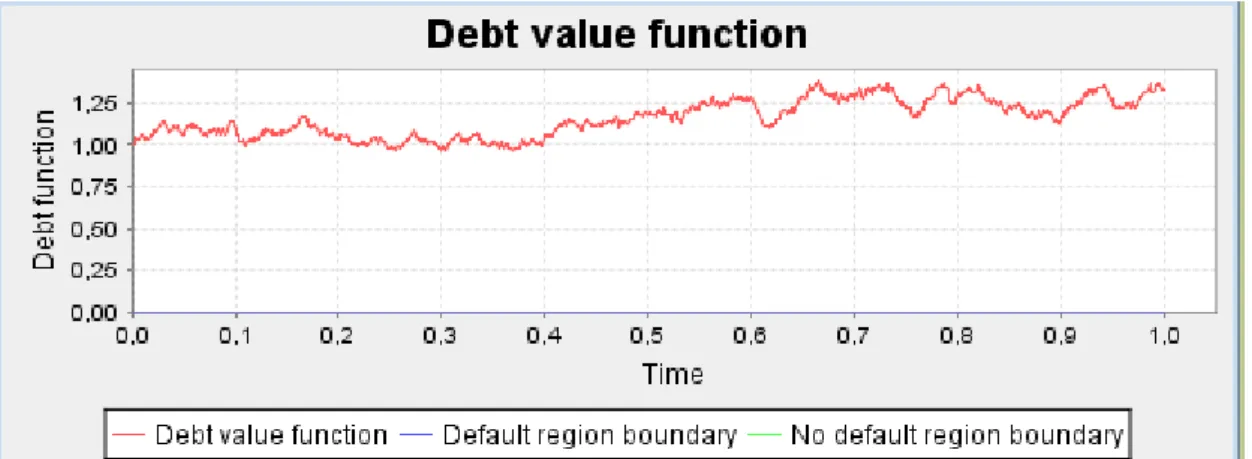
4.2.2. Debt function trajectory
Display the graphical lines representation of debt value function, default region boundary and no default boundary for one random trajectory calculated by the program.
X axis represent the time periods interval’s and y axis is debt value. Figure 33 below shown this
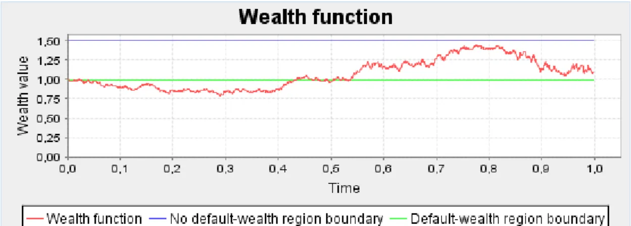
4.2.3. Wealth function
When the user click on wealth function label he or she will get Figure 34 below that display the graphical lines representation of wealth function, no default-wealth region boundary and de-fault wealth region boundary for one random trajectory calculated by the program.
X axis represent the time periods interval’s and y axis is wealth value.
Figure 34 wealth function
4.2.4. Risk investment function
By clicking investment labels in output panel, the user will have Figure 35 that illustrate the investment opportunities policies graphs, where lines represent risk investment functions for first and second opportunity. X axis represent the time periods interval’s and y axis is invest-ment values for each opportunity.
4.2.5. Numerical results
This panel demonstrates the numerical values calculated by the program. These values concern the default-wealth region boundary and no default-wealth region boundary which was used in figure 16 for wealth function. And the values of default region boundary and no default region boundary which have been used in Figure 33 for debt value functions.
Figure 36 display this panel
Figure 36 numerical results
If the user chooses default and wealth radio button and then click on start button in control panel he or she shall get the following:
4.2.6. Default Relative Frequency Histogram
This histogram represents the default trajectories simulated by the programs among the total numbers of trajectories chooses in input panel.
The code of calculating the numbers of histogram columns, as following:
int nbins1 = (int) Math.pow (defaultCounter, 0.333);
X axis represent the time periods interval’s and y axis is number of default trajectories in an interval. Figure 37 below illustrated this.
4.2.7. Wealth Relative Frequency Histogram
When the user click on wealth label in output panel she or he will get the wealth histogram as mentioned before.
The code of calculating the numbers of histogram columns, as following:
int nbins2 = (int) Math.pow (N, 0.333);
X axis represent wealth values intervals at maturity, time T, and y axis is number of wealth baths in an interval. Figure 38 shows that
Figure 38 wealth relative frequency histograms
4.2.8. Joint Histogram
Joint histogram represents the bivariate density of the borrower’s time –T optimal wealth, when debt maturity coincides with the borrower’s planning horizon with rela-tion to the default wealth trajectories. Figure 39 shows that
) (
*
T
W (T =T′)
Figure 39 joint histogram
4.2.9. Final Numerical Results
Here user can get almost all the necessary output of BasakShapiro2 models.
These outputs are useful in decisions making or problem analysis. The discretion of this output shown in figure 41 below
4.2.10. Risk Exposure function
To get the risk exposure function the just click on risk exposure function label’s in out panel where X axis represent time intervals and y axis is risk exposure value which calculated ac-cording to formula 14. As shown in Figure 40
Figure 40 risk exposure function
5. Conclusion
Our study is based on Basak-Shapiro model that aim to verify if the default costs, when default occurs, have an effect on the optimal decisions and polices of borrowers (firm or household) and analyzed the associated investment policies and implications for market dynamics.
In part 2 the study viewing Basak-Shapiro model approaches in modeling the debt contract and default costs when debt maturity coincides with planning horizon . In part 3 we introduce the study approaches for deriving the necessaries formulas for model outputs and others variables. The study design Java program to re-calculate, generally, with new approaches the various Outputs and variables needed for the model. Accordingly, we find that our Java program has the same results as Basak-Shapiro model calculations. In other words, it also shows that our program has a high flexibility and advantages that make it appropriate for credit risk model. The state price density process (ζ) figure out with the times periods, as a new methods of es-timation that adapted in this study, and redefined as a debt value function describing a change that it taking place between debt value and time periods. The graph of the debt function sup-plied with the calculation of non default region boundary(ζ*)and default region boundary
with almost compatible values as in Basak-Shapiro models. )
(ζ*
The borrower’s time-T, plus time-t, optimal wealth introduced in this study proportional with times periods and depicts in one compact graph and redefined as wealth function ,this in turn provided with no default-wealth region boundary
) ( * t W ) 1 ( ) ( * * β β ζ − = F W and default-wealth region boundary
[
]
⎭ ⎬ ⎫ ⎩ ⎨ ⎧ − + = ) 1 ( ) ( * * * β λ β ζ β ζ yW
I
. This technique differs than what have been used in Bask-Shapiro models. This is allowing end user to follow the graph of the functions, typically its values, through out times periods of debt contract until the maturity date of debt contract T. The same approach was used also in depicting risk investment functions, as repre-senting the investment opportunities, and risk exposure functionm*(t).As end user can easily change the inputs values of the Java program so he or she is able to see the effects of changing model parametersF,β,λ,φon borrower’s optimal wealth across the defaults regions and analysis the reasons of the probability of default at time state of the econ-omy.
Defaults probabilities were demonstrated with default histogram. Java program presents histo-grams of default of the model simulated trajectories.
Probability of default is estimated through the program, in addition to the mean and variance of the default. The program calculates also quartiles (10%, 25%, 50%, 75% and 90%) that aid end user to carry out the necessary statistic inferences needed for this model.
Java Program arranges wealth histograms of credit risk model. Borrower’s optimal value and wealth mean takes approximately same values when the numbers of simulated trajectories in-creases. Java program compute wealth variance and quartiles (10%, 25%, 50%, 75% and 90%)
those all indeed offer a helpful tool to make statistical inferences concern probabilistic interpre-tation of borrower’s optimal wealth at maturity date of debt contact.
Java program figure out risky investment opportunities functions with time period till maturity. The study concluded as a time headed for debt maturity threaten of default is very likely so the borrowers prefer risk less investments to the default and fulfill his obligations.
Then, we analyze the sensitivity of risk exposure function and exam the effects of changing the debt-contract parameters(F,β)default-costs parameters(Fφ,λ). These effects displayed graphically and numerically. We highlighted the different influence of variety types of cost and explained analytically how a borrower’s risk function may be seen.
We also pointed out how the probability of default vanishes or reduced with the extension of resistance region by changing default boundaries. These changes improve the borrower’s fi-nancial positions by reducing the risk and likewise default on fifi-nancial obligations.
Finally, we remember that our main objective was to build an applet for Basak-Shapiro model for estimating credit risk. After identifying our aims, we in advance to inspect the mathematical backdrop for model computation. This guide us to the conception of layout of our applet; we then utilize of Java library to build out the essential codes appropriate
For create the applet.
We then uphold that the objective of our study has been attained, and the user guide described in part 4 will assist the user recognize how the UI works. Up till now, we have never test the optimization when prehorizon default is allowed in this study. We recommended the others researchers to follow and complete this goal.
6. References
[1] Dempstar.M.A.H, Risk management: Value at risk and beyond, Cambridge University, Cambridge, 2002
[2] Jorion philippe, Value at risk: The new benchmark for managing market risk. 2nd ed. New York, McGraw-Hill, 2000
[3] Suleyman Basak and Shapiro Alexander, a Model of credit risk, optimal policies and asset
prices, journal of business, University of Chicago, Vol.78.no 4(2005), 1215-1266
[4] Jarrow. Robert A, Turnbull. S, Derivative securities, 2nd ed, South-Western College Pub-lishing, Ohio, 2000
[5] Hull.J.C, Option future and other derivatives.,6th ed. Upper Saddle River, NJ: Prentice Hall, 2006
[6] Dennis D. Wackerly, William M III, Richard L. Scheaffer, Mathematical statistics applica-tions., 6th ed, Duxbury and Book, 2002
[7] Campione, M., Walrath, K. and Huml, A. The Java TM tutorial: a short course on the
ba-sic, 3rd ed, The JavaTM Series, Addison Wesley, Upper Saddle River, NL, 2006
[8] Dimitrii, S., H., Jönsson and A. Malyarenko, How to write seminar reports and thesis, 2006 [9]Mathew. John H, Fink. Kurtis D, Numerical methods using MAT LAB., 4th ed , Person Pren-tice Hall, 2004
[10]Howard Anton, Chris Robres, Elementary linear algebra, 8th ed, John Wiley & Sons.Inc, 2000
7. Appendix
Java Code /**
* @(#) BasakShapiro.java 1.0 06/09/21 *
* Copyright (c) 2006 Mälardalen University
* Högskoleplan Box 883, 721 23 Västerås, Sweden. * All Rights Reserved.
*
* The copyright to the computer program(s) herein * is the property of Mälardalen University.
* The program(s) may be used and/or copied only with * the written permission of Mälardalen University * or in accordance with the terms and conditions * stipulated in the agreement/contract under which * the program(s) have been supplied.
*
* Description: Monte Carlo simulation of the state price * density process in Basak-Shapiro model
*
* Glasserman, P.
* Monte Carlo methods in financial engineering * Springer, Berlin, 2003
*
* @version 1.0 21 Sep 2006 * @author Basil Wakid Hassan * Mail:bwd0300@student.mdh.se */ import java.awt.*; import java.awt.event.*; import javax.swing.*; import javax.swing.border.*; import java.text.*; import java.util.*; import org.jfree.chart.*; import org.jfree.chart.axis.*; import org.jfree.chart.plot.*; import org.jfree.data.xy.*; import org.jfree.data.statistics.*; import org.freehep.j3d.plot.*;
public class BasakShapiro2 extends JApplet
implements FocusListener, ActionListener {
// class variables // panels
private JPanel mainPanel = null;
private JPanel inputPanel = null;
private JPanel dataPanel = null;
private JPanel controlPanel = null;
private ChartPanel debtPanel = null;
private ChartPanel wealthPanel = null;
private JPanel riskyPanel = null;
private ChartPanel investmentPanel = null;
private JPanel numericalPanel = null;
private ChartPanel riskExposurePanel = null;
//Labels
private JLabel retainingRateLabel = null;
private JLabel faceValueLabel = null;
private JLabel fixedCostLabel = null;
private JLabel proportionalCostLabel = null;
private JLabel interestRateLabel = null;
private JLabel debtContractMaturityLabel = null;
private JLabel driftCoefficient1Label = null;
private JLabel driftCoefficient2Label = null;
private JLabel volatility1Label = null;
private JLabel volatility2Label = null;
private JLabel volatilityCorrelationLabel = null;
private JLabel numberOfTrajectoriesLabel = null;
private JLabel numberOfTimesStepsLabel = null;
// labels for numerical panel
private JLabel defaultRigonBoundaryLabel = null;//1
private JLabel noDefaultRigonBoundaryLabel = null;//3
private JLabel defaultValueLabel = null;//5
private JLabel probabilityOfDefaultLabel = null;//7
private JLabel defaultMeanLabel = null;//9
private JLabel defaultVarianceLabel = null;//11
private JLabel defaultTenLabel = null;//13
private JLabel defaultTwentyfiveLabel = null;//15
private JLabel defaultFiftyLabel = null;//17
private JLabel defaultSeventyFiveLabel = null;//19
private JLabel defaultNinetyLabel = null;//21
private JLabel wealthPriorDebtMaturityLabel = null;//2
private JLabel optimalWealthLabel = null;//4
private JLabel probabilityOfOptimalWealthLabel = null;//6
private JLabel wealthMeanLabel = null;//8
private JLabel wealthVarianceLabel = null;//10
private JLabel wealthTenLabel = null;//12
private JLabel wealthTwentyfiveLabel = null;//14
private JLabel wealthFiftyLabel = null;//16
private JLabel wealthSeventyFiveLabel = null;//18
private JLabel wealthNinetyLabel = null; //20
//Text fields
private JTextField retainingRateField = null;
private JTextField faceValueField = null;
private JTextField fixedCostField = null;
private JTextField proportionalCostField = null;
private JTextField interestRateField = null;
private JTextField debtContractMaturityField = null;
private JTextField driftCoefficient1Field = null;
private JTextField driftCoefficient2Field = null;
private JTextField volatility1Field = null;
private JTextField volatility2Field = null;
private JTextField volatilityCorrelationField = null;
private JTextField numberOfTrajectoriesField = null;
// text fields for numerical panel
private JTextField defaultRigonBoundaryField = null;//1
private JTextField noDefaultRigonBoundaryField = null;//3
private JTextField defaultValueField = null;//5
private JTextField probabilityOfDefaultField = null;//7
private JTextField defaultMeanField = null;//9
private JTextField defaultVarianceField = null;//11
private JTextField defaultTenField = null;//13
private JTextField defaultTwentyfiveField = null;//15
private JTextField defaultFiftyField = null;//17
private JTextField defaultSeventyFiveField = null;//19
private JTextField defaultNinetyField = null;//21
private JTextField defaultWealthRegionBoundaryField = null;//2
private JTextField noDefaultWealthRegionBoundaryField = null;//4
private JTextField optimalWealthField = null;//6
private JTextField wealthMeanField = null;//8
private JTextField wealthVarianceField = null;//10
private JTextField wealthTenField = null;//12
private JTextField wealthTwentyfiveField = null;//14
private JTextField wealthFiftyField = null;//16
private JTextField wealthSeventyFiveField = null;//18
private JTextField wealthNinetyField = null;//20
// buttons
private JButton startButton = null;
// radio button group
private ButtonGroup group = null;
// radio buttons
private JRadioButton graphButton = null;
private JRadioButton defaultsButton = null;
// progress bar
private JProgressBar progressBar = null;
// tabbed panes
private JTabbedPane outputTabbedPane = null;
// the corresponding boolean variable
private boolean bGraph = true;
// Lego plot
private LegoPlot plot = null;
// String constants
private final String INPUT_LABEL = "Input";
private final String RETAININGRATE_LABEL = "Retaining rate";
private final String FACEVALUE_LABEL = "Face value";
private final String FIXEDCOST_LABEL = "Fixed cost";
private final String PROPORTIONALCOST_LABEL = "Proportional cost";
private final String INTERESTRATE_LABEL = "Interest rate";
private final String DEBTCONTRACTMATURITY_LABEL = "Debt contract
matur-ity";
private final String DRIFTCOEFFICIENT1_LABEL = "Drift coefficient 1";
private final String DRIFTCOEFFICIENT2_LABEL = "Drift coefficient 2";
private final String VOLATILITY1_LABEL = "Volatility 1";