Agent-based simulation fusion for improved decision making for service operations

http://www.diva-portal.org

Postprint

This is the accepted version of a paper presented at International Conference on Information Fusion,

Seattle, 06 Jul - 09 July, 2009..

Citation for the original published paper: Hilletofth, P., Ujvari, S., Johansson, R. (2009)

Agent-based simulation fusion for improved decision making for service operations.

In: Proceedings of the 12th International Conference on Information Fusion (pp. 998-1005). Seattle, US

N.B. When citing this work, cite the original published paper.

Permanent link to this version:

Proceedings of the 12th International Conference on Information Fusion (Seattle, WA)

Agent-Based Simulation Fusion for Improved Decision

Making for Service Operations

Per Hilletofth

Logistics Research Centre University of Skövde per.hilletofth@his.se

Sandor Ujvari

Logistics Research Centre University of Skövde sandor.ujvari@his.se

Ronnie Johansson

Informatics Research Centre University of Skövde ronnie.johansson@his.se

Abstract - We use agent-based modeling and simulation

to fuse data from multiple sources to estimate the state of some system properties. This implies that the real system of interest is modeled and simulated using agent principles. Using Monte-Carlo simulation, we estimate the values of some decision-relevant numerical properties. We use the estimated properties, such as utilization of resources and service levels, as a decision support for a Maintenance Service Provider. Our initial results indicate that this kind of fusion of information sources can improve the understanding of the problem domain (e.g. to what degree some critical properties influence service operations) and also generate a basis for decision-making.

Keywords: Agent-based simulation fusion, Service

operation, Agent-based modeling and simulation, Decision support.

1 Introduction

Outsourcing of maintenance involves the use of external companies, referred to as Maintenance Service Providers (MSP). MSPs can encompass the entire maintenance function or selected activities. Provided services can either be corrective, preventive or conditional [1]. MSPs are subject to a rapidly changing business environment strongly influenced by the Forrester Effect of non-stock production [2], and research has shown that information is vital in avoiding up and down swings in resource needs. Additionally, operations need to be well balanced in terms of utilization rate of personnel (hours billed divided by hours worked) versus service rate towards customers. Another important topic is to keep a balance between maintenance cost and the up-time of the customers’ production systems. MSPs also serve other customers in various geographical locations, and these can have long-term contracts for service levels.

One way to improve decision-making for MSPs to deal with the aforementioned topics is to generate business intelligence by exploiting business data from various available sources [3]. The decision support could consist of estimation of decision-relevant properties that relate to the performance of the MSP’s organization (i.e., properties which the decision maker has the opportunity to affect or which could provide improved understanding

of the business situation). The organization (or system, more generally) properties of interest inherently depend on the interactions (possibly random) of the components of the organization. Sources contain information about the customers as well as properties of the MSP’s own organization and the business environment (e.g., changing demand patterns, new market actors and suppliers’ performance).

Within the Information Fusion (IF) community, various methods for synergistic exploitation of multiple sources are being studied and developed. In fact, IF can be defined as “the study of efficient methods for automatically or semi-automatically transforming information from different sources and different points in time into a representation that provides effective support for human or automated decision making” [4]. Popular methods for fusing sources include various types of filtering [5], Bayesian networks [6], and evidential theory [7]. However, for the kind of problem we are considering here, the relationships between the business data and the decision-related properties are intricate and difficult to capture with the aforementioned methods. The filtering techniques, e.g., help to estimate the state of a dynamic system from observations. However, the system or organization properties that we study in our work should not be tracked and the decision-relevant system properties are not observed. Bayesian networks require that conditional probabilities between observation variables and decision-relevant variables can be specified, which are not always accessible (especially if the interrelations between different components of the system are complex). Evidential theoretical approaches require that evidences for decision-relevant properties can be specified which might be far from trivial. The alternative approach to fusion, which we use in this work, is agent-based modeling and simulation (ABMS). The ABMS approach allows us to model the components of the organization and estimate organization properties based on business data and simulations. The motivation for this approach is that for some problems and environments all decision-relevant properties are not known, and finding these is a part of the problem. These should be discovered during the modeling and simulation process. Using this approach the modeling process becomes iterative requiring high scalability and means for uncomplicated remodeling [8]. These are all features of ABMS.

Surprisingly, ABMS has, so far, received very little attention from the IF community (in spite of its seemingly close relation to impact assessment), unlike agent-based methods for distributed control [9] and information processing [10-11]. A notable exception is [12] who, without an explicit fusion perspective, use ABMS to evaluate the possible consequences of candidate plans.

In this research, an agent-based simulation model of service related maintenance has been developed. The simulation model is inspired by an actual case company, e.g. some random components of the model are gained from the case company, but additional data has also been used. Empirical data was collected during a three year period (2006-2008) from various sources including databases, interviews, observations, and internal documents. In the simulation model, the service order fulfillment process is managed by a set of agents that are responsible for one or more activities. It comprises a complex service network (more than 25 customer factories), which is modeled using one common type of industrial machine to be served. The remainder of the paper is structured as follows: In Section 2, the general concept of agent-based simulation for information fusion is presented. Thereafter, in Section 3 the MSP organization is presented. In Section 4, the simulation model for the MSP and some initial results are presented in Section 5. In Section 6, the research is concluded and further research avenues are proposed.

2 Agent-Based Simulation Fusion

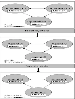
ABMS represents a new paradigm in modeling and simulation, especially suited to resemble complex and dynamic systems distributed in time and space [13]. It implies that the real system of interest is modeled in the form of a set of interacting agents within a certain environment (i.e. as an agent system) and implemented in simulation software, resulting in an agent-based simulation model (Figure 1).

An agent system consists of a set of individual agents with specified relationships to one another within a certain environment. The agents are presumed to be acting in what they perceive as their own interests, such as economic benefit (i.e. they have individual missions), and their knowledge regarding the entire system (i.e. other agents and environment) is limited [8]. Still, the most important feature of an agent system is the agents’ ability to collaborate, coordinate and interact with each other as well as with the environment to achieve individual and common goals [14]. By sharing information, knowledge, and tasks among the agents in the system, collective intelligence may emerge that cannot be derived from the internal mechanism of an individual agent. Furthermore, the ability to coordinate makes it possible for agents to coordinate their actions among themselves, i.e. taking the effect of another agent’s actions into account when making a decision about what to do.

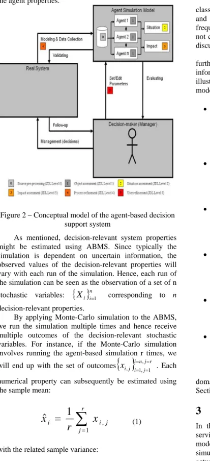
An agent-based simulation can be used to simulate the actions and interactions of system components to estimate the effects on the system as a whole as well as to evaluate decision-relevant properties of the system. This implies that an agent-based simulation can be used as a decision support system (Figure 2). The simulation basically consists of the interacting agents and some situation and impact variables. The utilized data in the simulation can be collected from databases and other sources representing the real system.

Figure 1 – The Process of agent-based modeling and simulation

Decision makers can set parameters in the simulation model, run the simulation and evaluate the results. Based on the retrieved information/knowledge they can make decisions regarding how to handle the real system. They could also continually alter different parameters and simulate again to evaluate different management alternatives. As a method for performing information fusion, ABMS permits the fusion of multiple information sources regarding a system of interest to estimate not easily accessible system properties. The information pertaining to the sources may be both known (e.g., customer data) and uncertain (e.g., machine failure). Random samples of the uncertain information may be used in a simulation run. The information may also be

historical and immediate. Historical data (e.g., previously

performed maintenance tasks) can be used, e.g., to estimate agent properties and interaction patterns. Immediate data concern rapidly changing properties of

simulation, e.g., the weather conditions, availability of spare parts. The information sources will in this way affect both the structure of the agent simulation (i.e., the types of agents and their interaction patterns) as well as the agent properties.

Figure 2 – Conceptual model of the agent-based decision support system

As mentioned, decision-relevant system properties might be estimated using ABMS. Since typically the simulation is dependent on uncertain information, the observed values of the decision-relevant properties will vary with each run of the simulation. Hence, each run of the simulation can be seen as the observation of a set of n stochastic variables:

{ }

X

_{i i}n₌₁ corresponding to n decision-relevant properties.

By applying Monte-Carlo simulation to the ABMS, we run the simulation multiple times and hence receive multiple outcomes of the decision-relevant stochastic variables. For instance, if the Monte-Carlo simulation involves running the agent-based simulation r times, we will end up with the set of outcomes

{ }

i n j r

j i j i

x

=₌ ,₌= 1 , 1 , . Each

numerical property can subsequently be estimated using the sample mean:

∑

=

=

r j j i i

x

r

x

1 ,

1

ˆ

₍₁₎

with the related sample variance:

(

)

∑

=

−

−

=

r j i j i i

x

x

r

s

1 2 , 2

ˆ

1

1

ˆ

(2)

Categorical properties (i.e., properties which are classes rather than numerical) could also be considered and the analysis could involve estimating their relative frequency. Categorical properties are, however, currently not considered for our application and will not be further discussed in the paper.

A conceptual model of the generic ABMS, which further relates ABMS (with Monte-Carlo simulation) to information fusion, is shown in Figure 2. The figure illustrates how the levels of the information fusion JDL model [15] can be interpreted in ABMS.

• Level 0 – Source pre-processing – is performed when real system data is adapted to the simulation model. This involves, e.g., dealing with missing data and adapting data to the requirements of the agent simulation.

• Level 1 – Object assessment – is performed when real system properties are being estimated for use in the simulation, e.g., estimating the capabilities and interaction protocols of agents from data • Level 2 – Situation assessment – is performed

when the situation variables are estimated from the simulation, e.g., the performance of agents in a manufacturing simulation

• Level 3 – Impact assessment – is performed when parameters concerning future effects are considered, e.g. risks to business venture or threats to a military campaign

• Level 4 – Process refinement – is performed when the simulation model is updated or the set of data the simulation is based upon is changed

• Level 5 – User refinement – is performed when the user sets parameters, runs different simulation scenarios, and evaluates the results, iteratively In the following section, we describe the problem domain of a MSP and present our simulation model in Section 4.

3 Research Environment

In this research, an agent-based simulation model for service related maintenance has been developed. The model has been implemented using leading agent-based simulation software named Anylogic. It is inspired by an actual case company, but additional data has also been used. The case company tries to manage all customer

orders and inquiries through a service central. The service central primarily works with orders and inquiries concerning operative maintenance. These types of orders stand for a big share of the total amount of orders. However, the service central also answers questions concerning product and service assortment and guide customer in the organization. Only maintenance coordinators are connected to the service central, which implies that a customer asking for other services is further guided in the organization. Customer orders and inquiries concerning other services than operative maintenance go through the sales department, which handles customer contacts and communicates with different coordinators in the organization. The maintenance coordinators are responsible for the weekly maintenance planning as well as for day-to-day planning. This implies that they determine which technicians that should be assigned to which tasks. Currently, the organization is divided into two divisions, mechanical and electrical maintenance. The engineers who belong to the two divisions are responsible for conducting the tasks and also reporting what have been done. Currently the reported information mostly concerns information for invoicing. The case company has identified the service fulfillment process and its management to be one of the most important improvement areas. It has been recognized that there is a need to change the service organization. The company wants to manage all orders and inquiries, irrespective of type, through a sales and service central in order to make the operations more efficient (optimize resource utilization) and more effective (enhance turnover and profits). Essentially, it‘s about enhancing the planning of maintenance services, which in a recently completed customer questionnaire has been ranked as one of the case company’s most important improvement areas. The company is, however, not clear on how the sales and service central should be structured and managed. One discussed solution is to enlarge the current service central’s responsibilities in order to create a centralized order entrance handling the entire product and service assortment. The sales and service central should store, collect, and fuse information to provide appropriate decision support. Information can be gathered from customers (customer information, service needs, location of target/problem, information about target/problem), simulations (simulate “what-if” scenarios), databases (customer information concerning system, equipment and what that have been done earlier) and staff (skills, utilization, working radius) to support decisions concerning needed maintenance services.

4 Simulation Model

The simulation model is inspired by an actual case company. For instance, some random components are gained from service times, travel times, demand types and operating structure of the case company. However,

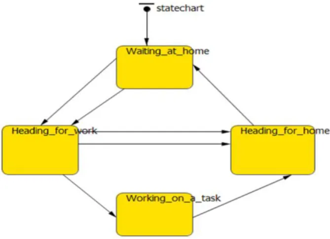
additional data has been used to allow the simulation model to be developed. Empirical data was collected during a three year period (2006-2008) from various sources including databases, interviews, observations, and internal documents. The sources contain information such as: operation structure, customer locations, service times, travel times, demand types and type of maintenance tasks. The simulation model contains two kinds of agents: engineers and tasks. Each task requires a finite time to be completed and the individual engineers work on these tasks. Both kinds of agents send a lot of messages to each other in order to inform about changes in their states. There are two types of engineers: mechanical and electrical engineers. In this model, each task requires one type of engineers to work on them, e.g. an electrical engineer cannot work on a task which requires the skills of a mechanical engineer. Also, the engineers have further been divided to engineers working on corrective tasks and to engineers working on planned tasks. Thus, there are four different types of engineers in the model and their numbers can be altered. Each engineer has four different states: waiting at home, heading for a task, working on a task, and heading home (Figure 3). The engineers start at their home location and wait for a task to arrive; when it does they will change their state to “heading for a task”. As soon as the engineer reaches its target, it will change its state to “working on a task”. At the same time, the engineer will send a message to the task to inform that it is being worked on. The engineer will work on the task until it receives a message from the task. When the message arrives, the state changes to “heading for home” and it will further change to “waiting at home” as soon as the engineer arrives at home.

Figure 3 – State chart for engineer agents

There are two types of tasks: corrective and planned. The locations of the tasks have been predefined and there are 28 different locations where they can occur. The corrective tasks occur unexpectedly while the planned tasks are planned well-ahead of their occurrence. The generation of both corrective and planned tasks is

extracted from real task data for reality. In the model the task lengths and frequency of occurrence are however estimations. Table 1 provides information on how corrective tasks are generated in the model. A new corrective task is generated between 4 to 12 hours, uniformly distributed. The corrective task generated will only contain one sub-task, i.e. require only one visit from an engineer (or engineers). The duration of the visit is normally distributed with a mean value of 2.8 hours and a standard deviation of 5 hours (each task will always have a positive length). 75% of corrective tasks require a mechanical engineer.

Each planned task is generated every 10 to 30 hours, uniformly distributed. Unlike the corrective tasks, planned tasks can have anything between 1 to 3 sub-tasks and the length for each sub-task comes from a normal distribution with a mean value of 10 and a standard deviation of 5. There will always be at least one task, but there is a 50% chance to have a second task. If there is a second sub-task, a third one will also have a 50% chance of occurring. A planned task will also have a randomized preferred starting date. In planned tasks each engineer has a schedule for two weeks. When a new planned task is generated, the total length of the task is used to fit the task to a free time-slot. The time-slots will be checked one at a time for each engineer so the actual starting date will not be minimized. If a planned task cannot be fitted to any of the engineers, the planned will be tried to be fitted at a later time (each hour in the model). If there is more than one unscheduled planned task, the shorter one will “steal” a time-slot from the longer one. This is because there will be a free slot earlier for a smaller task. This does not reflect reality well, but it is only an initial model.

Both corrective and planned tasks have only three states. The first one, “corrective situation”, only initiates the agent. Immediately after this the state changes to “Backlog” which is used to calculate the time waited for service. As soon as the first engineer arrives, the state is changed to “being worked on”. Figure 4 shows an example of the states in a corrective task.

Figure 4 – State chart for corrective task agents

Corrective tasks can be allocated to the engineers in two ways; as soon as a new corrective task is generated, each of the right type of engineers will inform whether they are working on a task or not. If there are no available engineers, the task will go to a queue to wait for an engineer to become available. If the amount of available engineers is higher than the amount of corrective tasks to be worked on (in queue plus new tasks) more than one engineer will be assigned to the task. However, when this happens, each task waiting for work will always have at least one engineer assigned to it. The engineers will also look for a task as soon as they arrive at home if they do not already have an assigned task. The heuristics is the same, e.g. there might be more than one engineer to be sent to a task. It is also possible that the customer gives incorrect information about the required task and the wrong type of engineer is sent to the task first. As soon as the “wrong” engineer arrives at the location, he immediately notices that he is not capable of completing the task. The engineer will then head home and the task is then given to the other types of engineers. When the first engineer arrives (right type or wrong type) the waiting time will be reported. Overall there are a lot of different variables which can be altered to study the behavior of the model and these are summarized in Table 1. The first four variables only show how many engineers exist in the model. The rest of the variables are random model components. Overall, the simulation model has a lot of randomness and each simulation run differs greatly from the previous ones. Thus, the model should be used for a Monte Carlo analysis in order to get more accurate results, also using a number of different seed values.

Table 1 – Variables inside the simulation model.

Variable Current values

Number of corrective electrical engineers 3 Number of corrective mechanical engineers 3 Number of planned electrical engineers 2 Number of planned mechanical engineers 3

Time between corrective tasks 4 – 12 hours, uniformly distributed Time between planned tasks 10 – 30 hours, uniformly distributed Length of planned tasks Mean: 10 hours, standard deviation 5 hours Length of corrective tasks Mean: 2.8 hours, standard deviation 5 hours Chance of ordering the wrong engineer 10 percent

The statistics that are recorded in the simulation model are presented in Table 2. These decision-relevant properties or indicators provide a situation image of the system’s overall performance (situation indicators) and can also highlight risks in the system, e.g. if the values are higher/lower than expected or wanted (impact indicators). Table 2 – Statistics gathered from the simulation model.

Statistics

Amount of kilometers driven

Amount of hours waiting for service at each customer location Amount of corrective tasks at each customer location Amount of hours spent working on a task Amount of hours spent moving Amount of hours spent waiting at home

Most of the statistics (given by Equation 1 and 2) can be calculated using the summarized time spent in different states of the agents. The time spent waiting, moving and working on a task can directly be calculated with the amount of agents each hour at each state. Also, the amount of hours waiting for service can be calculated with the amount of corrective tasks in “Backlog” state and amount of tasks at each location with the amount of tasks in “corrective situation” state. The last one, the amount of kilometers driven, is calculated with the help of state transitions in the engineer agents.

5 Simulation Results

The simulation model has a graphical view (Figure 5): the red stick-figures are electrical engineers while the mechanical ones are cyan. The crosses are corrective tasks while the circles are planned tasks.

Figure 5 – The main view of the simulation model. As the model contains a lot of random components, a Monte-Carlo analysis should be used to estimate the results of the model. In the Monte-Carlo analysis the same statistics were followed as in Table 2. The total amount of hours waited for service was divided by the amount of tasks at individual locations and this statistics indicates the average waiting time for each task. Most of the statistics is presented in Table 3 while Figure 6 shows an example of one of these statistics.

Table 3 – The results for the most important variables.

Variable Mean Standard deviation

Engineers waiting 52.2% 2

Engineers moving 21.6% 1.1

Engineers working 26.2% 1.4

Total kilometers driven 37 781 km 1 979 Corrective waiting time 5.14 hours 0.68

Figure 6 – Engineers waiting (ratio of available working

hours).

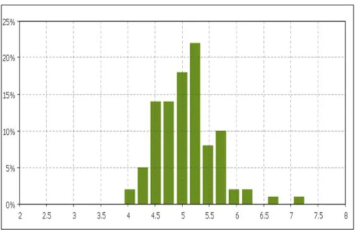
On average the engineers have to wait for work 52% of their time. Only 26% of their total working time is used on the actual value adding time of servicing while 22% is spent of moving between locations. As the engineers have to spend much time traveling between locations, the amount of kilometers driven has a strong impact on the profitability of individual customers. Figure 7 shows the average amount of kilometers driven. The mean value is 37781 kilometers and the amount of standard deviation is 1979 kilometers.

Figure 7 – Kilometers driven

The final statistics, average waiting time overall and at each individual location, mean value depends on a lot of different things. Each individual task’s waiting time does not depend solely on the location but also from the availability of the engineers. This, on the other hand, is dependent on the location of the previous tasks and their lengths. Also, if a wrong engineer is sent to a corrective task, a lot of time is wasted. These waiting times are presented in Figures 8 and 9.

Figure 8 – Average waiting time for customer (hours)

Figure 9 – Average waiting time for customer in individual locations (hours)

As it can be noticed from Figure 9, the average waiting time on individual locations differs a lot. It should be noted that even in the town, where the MSP is located, the average waiting time is three hours, despite the fact that the engineers spend 50% of their time waiting for tasks. This can be expected, when the rate of corrective tasks is relatively high with respect to planned tasks. Figure 9 can also be used to estimate the availability promised to customers.

6 Discussion and Conclusions

For some problems and environments all decision-relevant properties are not known, and finding these is a part of the problem. Since these can be discovered during the modeling and simulation process we have shown that an effective decision support system for MSPs can be developed using agent-based simulation fusion. The simulation model enables decision makers to set parameters, run the different simulation scenarios and evaluate the results, iteratively and to evaluate different management alternatives. Based on the retrieved information/knowledge they can make decisions regarding, how to handle the real system. The results of

this research are twofold: in part relating to the application domain, and in part relating to the use of ABMS for information fusion.

Some conclusions can be drawn about the problem domain based on this work. These conclusions should be considered in light of the validation of the model; since some data is not available before the real system estimations have been made. However, these have been evaluated by application domain experts and the behavior of the model does not show any unrealistic properties. Still, the performance results presented here are not necessarily representative over time for the investigated MSP; with improved input data this could improve significantly. The simulation research findings reveal that response lead time in corrective maintenance varies greatly based on two factors, namely the amount of needed resources, and the travel time. Demand itself is relatively easy to manage since typically only one maintenance engineer visit is required when service is actually needed. However, in planned maintenance, demand management has a more significant role, since more than one visit on site is typically needed, and the predictability of the number of visits as well as maintenance hours is larger. As the maintenance operator uses a centralized service structure (all resources in one location), considerable amount of time and accumulated costs are tied in traveling to the customer sites. Our simulation experiment shows that management of travel times and costs should receive attention and also that the centralized service strategy should be evaluated. A closer study and monitoring of performance and costs can in the future motivate a more decentralized structure.

Based on these results it can be argued that the agent-based simulation fusion has improved the understanding of the problem domain (i.e. maintenance planning) and also generated a basis for decision-making. ABMS fusion has so far not been well explored but provides an intriguing way of considering information sources and fusing them. One challenge for future research is to characterize the types of problems for which ABMS fusion is necessary and cannot be replaced by simpler approaches. Another challenge is how to evaluate the reliability of the agent simulation. It will have to be dependent on the validity of the simulation model. A third challenge is to combine the result of the ABMS fusion with other sources.

These results should be generic for other types of service organizations since the problem of achieving a high customer service rate and a high utilization rate is inherently difficult in low-beforehand demand information contexts (e.g. some instances of taxi-operations, ambulance etc). The results of using this type of simulation approach is twofold; i) it is possible, once the simulation is validated, to test the outcome of different settings to find a balance between e.g. customer service rate and utilization rate, the result of new locations on the ratio travel-time and work-time at customers, ii) estimate

and motivate the actual value of increased data gathering and information generation in most parts of the work process, e.g. service reports, customer production data etc.

References

[1] A. Garg, and S.G. Deshmukh, “Maintenance management: literature review and directions”, Journal of

Quality Maintenance Engineering, Vol. 12, pp. 205-238,

2006.

[2] H. Akkermans, and B. Vos, “Amplification in service supply chains: an exploratory case study from the telecom industry”, Production and Operations

Management, Vol. 12, pp. 204-223, 2003.

[3] P. Hilletofth, S. Ujvari, and O.-P. Hilmola, “Information Fusion in Maintenance Planning”,

Proceedings of the Swedish Production Symposium,

28-30 August, Göteborg, 2007

[4] H. Boström, S.F. Andler, M. Brohede, R. Johansson, A. Karlsson, J. van Laere, L. Niklasson, M. Nilsson, A. Persson, and T. Ziemke, On the Definition of Information

Fusion as a Field of Research, Technical Report

HS-IKI-TR-07-006, Informatics Research Centre, University of Skövde, 2007.

[5] S. Blackman, and R. Popoli (1999), Design and

analysis of modern tracking systems, Artech House,

ISBN: 1-58053-006-0.

[6] S. Das, High-level data fusion, Artech House, ISBN: 978-1-59693-281-4, 2008.

[7] G. Shafer, A mathematical theory of evidence, Princeton University Press, 1976.

[8] C.M. Macal, and M.J. North, “Tutorial on agent-based modeling and simulation part 2: how to Model with Agents”, Proceedings of the Winter Simulation Conference, 2006

[9] G.M. Mathews, and H. F. Durrant-Whyte, “Scalable decentralised control for multi-platform reconnaissance and information gathering tasks”, Proceedings of the 9th

International Conference on Information Fusion, 2006.

[10] M. Brännström, R. Lennartsson, A. Lauberts, H. Habberstad, E. Jungert, and M. Holmberg, “Distributed data fusion in a ground sensor network”, Proceedings of

the 7th International Conference on Information Fusion,

pp. 1096—1103, 2004

[11] D. Perugini, D. Lambert, L. Sterling, and A. Pearce, “Distributed information fusion agents”, Proceedings of

the 6th International Conference on Information Fusion,

pp. 86-93, 2003.

[12] Q. Huang, J. Hållmats, K. Wallenius, and J. Brynielsson, “Simulation-based decision support for command and control in joint operations”, Proceedings of

the 2003 European Simulation Interoperability Workshop,

number 03E-SIW-091, pages 591-599, Stockholm, Sweden, June 2003.

[13] M.K. Lim, and Z. Zhang, “A multi-agent based manufacturing control strategy for responsive manufacturing”, Journal of Materials Processing Technology, Vol. 139, No. 1/3, pp. 379-384, 2003.

[14] P. Hilletofth, T. Aslam, O.-P. Hilmola, “Multi-Agent based Supply Chain Management: Case Study of Requisites”, International Journal of Networking and

Virtual Organisations, forthcoming 2009.

[15] J. Llinas, C. Bowman, G. Rogova, A. Steinberg, E. Waltz, and F. White, “Revisiting the JDL Data Fusion Model II”, Proceedings of the 7th International

Conference on Information Fusion, pp. 1218-1230,