This is the published version of a paper published in International Journal of Distributed Sensor
Networks.
Citation for the original published paper (version of record):
Ahmad, N., Khursheed, K., Imran, M., Lawal, N., O'Nils, M. (2013)
Modeling and Verification of a Heterogeneous Sky Surveillance Visual Sensor Network.
International Journal of Distributed Sensor Networks, : Art. id. 490489
http://dx.doi.org/10.1155/2013/490489
Access to the published version may require subscription.
N.B. When citing this work, cite the original published paper.
Permanent link to this version:
Volume 2013, Article ID 490489,11pages http://dx.doi.org/10.1155/2013/490489
Research Article
Modeling and Verification of a Heterogeneous Sky Surveillance
Visual Sensor Network
Naeem Ahmad, Khursheed Khursheed, Muhammad Imran,
Najeem Lawal, and Mattias O’Nils
Division of Electronics Design, Mid Sweden University, Holmgatan 10, 851 70 Sundsvall, Sweden
Correspondence should be addressed to Naeem Ahmad; naeem.ahmad@miun.se Received 19 April 2013; Accepted 29 July 2013
Academic Editor: Ivan Lee
Copyright © 2013 Naeem Ahmad et al. This is an open access article distributed under the Creative Commons Attribution License, which permits unrestricted use, distribution, and reproduction in any medium, provided the original work is properly cited. A visual sensor network (VSN) is a distributed system of a large number of camera nodes and has useful applications in many areas. The primary difference between a VSN and an ordinary scalar sensor network is the nature and volume of the information. In contrast to scalar sensor networks, a VSN generates two-dimensional data in the form of images. In this paper, we design a heterogeneous VSN to reduce the implementation cost required for the surveillance of a given area between two altitude limits. The VSN is designed by combining three sub-VSNs, which results in a heterogeneous VSN. Measurements are performed to verify full coverage and minimum achieved object image resolution at the lower and higher altitudes, respectively, for each sub-VSN. Verification of the sub-VSNs also verifies the full coverage of the heterogeneous VSN, between the given altitudes limits. Results show that the heterogeneous VSN is very effective to decrease the implementation cost required for the coverage of a given area. More than 70% decrease in cost is achieved by using a heterogeneous VSN to cover a given area, in comparison to homogeneous VSN.
1. Introduction
Visual sensor networks (VSNs) are the image sensor based distributed systems. They consist of a large number of low-power camera nodes which collect image data from environ-ment and perform distributed and collaborative processing on this data [1, 2]. These nodes extract useful information from collected images by processing the image data locally and also collaborate with other neighboring nodes to create useful information about the captured events. The large amount of image data produced by camera nodes and the limited network resources demand the exploration of new techniques and methods of sensor management and processing and communication of large data. It demands interdisciplinary approach with the disciplines such as vision processing, communication, networking, and embedded processing [3]. Camera sensor nodes with different types and costs are available in the market today. These nodes have different optical and mechanical properties. They have varied ranges of computation capabilities, communication powers, and energy requirements. The choice of camera nodes to
design a VSN depends on the requirements and constraints of a given application. Depending on the type of the camera nodes, VSNs can be divided into two major categories, homogeneous and heterogeneous VSNs [4]. A homogeneous VSN uses similar types of nodes while a heterogeneous VSN uses different types of nodes.
VSNs have a large number of potential applications. They can be used in surveillance applications for intrusion detec-tion, building monitoring, home security, and so forth. These applications capture images of the surroundings and process them for recognition and classification of the suspicious objects [5,6]. Visual monitoring is being used in retail stores and in homes for security purposes [7]. Modern VSNs can provide surveillance coverage across a wide area, ensuring object visibility over a large range of depths [8,9]. They can be used in traffic monitoring applications [10–14] for vehicle count, speed measurements, vehicle classifications, travel times of the city links, and so forth. VSNs have a number of applications in sports and gaming field [15,16]. They can collect statistics about the players or the game to design more specific training to suit the individual players. VSNs have
applications in environment monitoring to collect data about animals and the environment which can be helpful to solve the nature conservation issues [17, 18]. Video monitoring has important applications in searching empty parking lots [19]. The PSF application [20] is designed to locate and direct a driver to the available parking spaces, near a desired destination. Video tracking techniques are used for people tracking [21].
A homogeneous VSN is formed by combining similar camera nodes. In contrast to this, a heterogeneous VSN contains different types of nodes [4, 22]. A heterogeneous VSN provides many advantages over homogeneous VSN such as resolution of conflicting design issues, reduction in energy consumption without degrading surveillance accu-racy, higher coverage, lower cost, and reliability. The tasks allocation strategy in heterogeneous VSNs is designed such that the simpler tasks are assigned to resource-constrained nodes while more complex tasks are assigned to high per-formance nodes. For example, in a surveillance application, a motion detection task can be assigned to lower-resolution nodes while object recognition task can be assigned to high-resolution nodes. This strategy results in optimized use of node resources. This optimization in heterogeneous VSNs results in maximization of network lifetime as compared to homogeneous VSNs. In designing homogeneous VSNs, the sensor selection and node design are finalized on the basis of most-demanding application tasks. Assigning such a node to simpler tasks wastes precious node resources. A homogeneous VSN design is unable to provide all the desired features, such as higher coverage, low cost, reliability, and energy reduction, at the same time. It optimizes one or more parameters at the expense of other parameters [9,23].
A single camera has limited field of view and is unable to provide coverage of a large area. To cope with this problem, arrays of cameras are used. The decreasing cost and increasing quality of cameras have made the visual surveillance of an area common by using a network of cameras [24]. An important research area is the placement of visual sensors to achieve a specific goal. A common goal is to place the image sensors in the arrays for complete coverage of a given area. The other goal can be to minimize the cost of visual sensor arrays, while maintaining the required resolution. Currently, the designers place cameras by hand due to the lack of theoretical research on planning visual sensor placement. In future, the number of cameras in smart surveillance applications is expected to increase to hundreds or even thousands. Thus, it is extremely important to develop camera placement strategies [25,26]. In recent years, a large number of smart camera networks are deployed for a variety of applications. An important design issue in these distributed environments is the proper placement of cameras. Optimum camera placement increases the surveillance coverage and also improves the appearance of objects in cameras [24].
This paper discusses the design of a heterogeneous VSN, to be used for application of monitoring large birds, such as eagle, in the sky. The heterogeneous VSN will be able to provide coverage of each point in the area with the required minimum resolution. The heterogeneous VSN is designed by combining three sub VSNs for the surveillance
of an area between two altitude limits. The VSN will be implemented with real monitoring nodes, which will be designed by following the model. Images will be captured and measurements will be performed to verify the full coverage at the given lower altitude and minimum achieved resolution at the given higher altitude. The heterogeneous VSN will reduce the implementation cost in comparison to homogeneous VSN.
The remaining of this paper is organized as follows.
Section 2describes the necessary theory for designing homo-geneous and heterohomo-geneous VSNs. Section 3 discusses the camera models and optics used in the experiment.Section 4
describes the heterogeneous VSN coverage model.Section 5
discusses the experimental measurement performed to verify VSN parameters.Section 6discusses the results, and finally
Section 7describes the conclusion.
2. Theory
This section describes a brief theory about designing VSNs and discusses the homogeneous and heterogeneous VSN models. The heterogeneous VSN is a combination of a number of homogeneous VSNs and is effective in reducing the implementation cost for the surveillance of an area. An example of heterogeneous VSN is presented, and cost com-parison between homogeneous and heterogeneous VSNs is made to see the cost reduction capability of the heterogeneous VSN.
2.1. Homogeneous VSN Model. The design of a VSN for the
surveillance of golden eagles is presented in [27]. The VSN is formed with a number of cameras. A 3D visualization of the coverage with a matrix of cameras is shown inFigure 1. A sharp tip at the bottom of the figure represents a camera node. A number of such nodes form a matrix which is used to monitor eagles in the sky between two altitude limits above the ground, the higher altitude𝑎ℎand the lower altitude𝑎𝑙. The area covered by the VSN is increased as the altitude from the camera nodes is increased. The area coverage increases till lower altitude𝑎𝑙, where VSN is able to fully cover a given area. Above altitude𝑎𝑙the coverage starts to overlap. This overlap is used to apply triangulation technique to find the exact size and altitude of an eagle.
As the altitude of an eagle is increased from camera nodes, the resolution of its image on the camera sensor is decreased. A minimum image resolution is necessary to recognize an object moving at altitude𝑎ℎand is assumed to be 10 pixels per meter. For altitudes higher than𝑎ℎ, the resolution of the object image drops below the minimum required criterion, so the VSN coverage is assumed zero above this altitude. The dark surface at the top ofFigure 1represents the altitude𝑎ℎ.
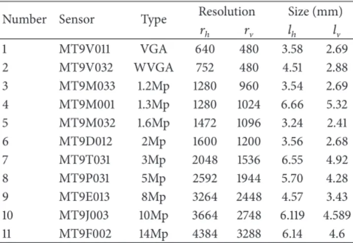
The first step to design a VSN is the selection of a camera sensor. A number of camera sensors are used in this study, and the details about their type, resolution, and size are given inTable 1. The second step of VSN design is the calculation of focal length of lens to be used with the chosen camera, which
Overlap Coverage Camera nodes L ower altitude Higher altitude dx dy
Figure 1: 3D visualization of coverage with a matrix of cameras.
Table 1: Camera sensors used in study.
Number Sensor Type Resolution Size (mm)
𝑟ℎ 𝑟V 𝑙ℎ 𝑙V 1 MT9V011 VGA 640 480 3.58 2.69 2 MT9V032 WVGA 752 480 4.51 2.88 3 MT9M033 1.2Mp 1280 960 3.54 2.69 4 MT9M001 1.3Mp 1280 1024 6.66 5.32 5 MT9M032 1.6Mp 1472 1096 3.24 2.41 6 MT9D012 2Mp 1600 1200 3.56 2.68 7 MT9T031 3Mp 2048 1536 6.55 4.92 8 MT9P031 5Mp 2592 1944 5.70 4.28 9 MT9E013 8Mp 3264 2448 4.57 3.43 10 MT9J003 10Mp 3664 2748 6.119 4.589 11 MT9F002 14Mp 4384 3288 6.14 4.6
ensures the minimum required resolution at altitude𝑎ℎand can be calculated by the following equation:
𝑓 = 𝑝𝑥 𝑙𝑥 ⋅ 𝑙ℎ 𝑟ℎ ⋅ 𝑎ℎ 𝑜r 𝑓 = 𝑝𝑦 𝑙𝑦 ⋅ 𝑙V 𝑟V ⋅ 𝑎ℎ, (1)
where𝑝𝑥and𝑝𝑦are the minimum number of pixels of the object image along width and length, 𝑙𝑥 and 𝑙𝑦 are width and length of the object,𝑎ℎis the higher altitude,𝑙ℎ and𝑙V are the image sensor lengths, and 𝑟ℎ and 𝑟V are the image sensor resolutions along horizontal and vertical directions, respectively. The angle of view (AoV) of a node, using a particular image sensor and a lens of specific focal length, can be calculated by the following equation:
𝛼 = 2 arctan 𝐾
2𝑓, (2)
where𝐾 is the chosen length (horizontal, vertical, or diago-nal) of the camera sensor and𝑓 is the lens focal length. The combination of camera and lens forms an individual node, and a number of such nodes are required to surveil a given area.
The third step of VSN design is the placement of nodes which ensures full coverage at the given lower altitude𝑎𝑙. The placement of nodes is calculated by calculating the distances 𝑑𝑥and𝑑𝑦between the two neighboring nodes, along𝑥 and 𝑦
directions, respectively. These distances can be calculated by the following equations:
𝑑𝑥= 𝑎𝑙𝑓⋅ 𝑙ℎ, 𝑑𝑦= 𝑎𝑙𝑓⋅ 𝑙V. (3) The fourth step of VSN design is to calculate the total number of nodes𝑛 (called cost) to cover a given area. The cost to cover a given area𝐴, can be calculated by the following equation:
𝑛 = 𝐴
(𝑙V/𝑙ℎ) ⋅ ((𝑎𝑙⋅ 𝑟ℎ⋅ 𝑙𝑥) / (𝑎ℎ⋅ 𝑝𝑥))2, (4) where𝑙ℎand𝑙V,𝑟ℎ,𝑟V,𝑝𝑥,𝑙𝑥,𝑎𝑙, and𝑎ℎare as defined above.
By using camera sensors given inTable 1 and the equa-tions from (1) to (4), a VSN can be designed to cover a given area in the given altitude ranges. The favorable VSN design objective is to increase the coverage of an area but decrease its implementation cost. However, in actual practice, the cost of a VSN is greatly increased when the covered area is increased. For example, to cover an area of 1 km2, between altitude limits from 3000 to 5000 m above the ground, a homogeneous VSN requires a cost of 20 nodes. This cost calculation assumes minimum resolution of 10 pixels per meter and 14 Mp camera sensor. If the area of 1 km2 is increased by extending the altitude limits from 500 to 5000 m, the cost of the VSN is increased to 694. In this example, the increase in area is about 2.25 times, but the corresponding increase in cost is about 35 times. This result indicates the need for a new technique which is able to increase the area coverage but at the same time decreases the implementation cost. In the following paragraphs the design of a heterogeneous VSN is presented which fulfills this purpose.
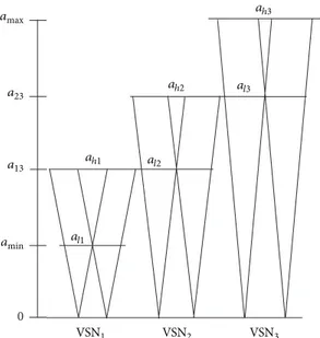
2.2. Heterogeneous VSN Model. The input parameters to
design a heterogeneous VSN include the area𝐴 to be covered, lower altitude𝑎𝑙, higher altitude𝑎ℎ, and the object size, 𝑙𝑥 and𝑙𝑦, to be monitored. The VSN is designed with three sub-VSNs: VSN1, VSN2, and VSN3, as shown in Figure 2. The VSN1is designed for lower altitude𝑎𝑙1and higher altitude𝑎ℎ1 and covering the top most part of the given altitudes range, the VSN2is designed for lower altitude𝑎𝑙2and higher altitude 𝑎ℎ2and covering the middle part of the given altitudes range, and the VSN3 is designed for lower altitude𝑎𝑙3 and higher altitude𝑎ℎ3and covering the lower part of the given altitudes range.
The given higher altitude 𝑎ℎ is treated as the higher altitude𝑎ℎ1 for VSN1. Suppose an image sensor𝑆1, having parameters𝑙ℎ1, 𝑙V1,𝑟ℎ1, and𝑟V1, is chosen to implement the nodes for VSN1along with a lens of focal length𝑓1. The lens focal length must ensure the minimum required resolution for the given object, when moving at the altitude 𝑎ℎ1. The value of𝑓1 can be calculated by using (1) for sensor𝑆1 and altitude𝑎ℎ1.
The VSN2 is designed to cover an area 𝐴 between the higher altitude 𝑎ℎ2 and the lower altitude 𝑎𝑙2. Suppose an image sensor𝑆2, having parameters 𝑙ℎ2, 𝑙V2, 𝑟ℎ2, and 𝑟V2, is chosen to implement the nodes for VSN2along with a lens
0 ah1 ah2 ah3 al1 al2 al3 amin a13 a23 amax VSN1 VSN2 VSN3
Figure 2: Heterogeneous VSN model.
of focal length𝑓2. The value of the altitude𝑎ℎ2, where the combination of the sensor𝑆2and the lens of focal length𝑓2 can provide the minimum required resolution for the given object, can be derived from (1) and is given below:
𝑎ℎ2=𝑝𝑙𝑥 𝑥 ⋅
𝑟ℎ2
𝑙ℎ2 ⋅ 𝑓2. (5) The VSN2 will cover the altitudes range from 𝑎ℎ2 and below. The VSN1 must ensure the coverage of the altitudes range from𝑎ℎ1to𝑎ℎ2. The higher altitude𝑎ℎ2for VSN2will serve as the lower altitude𝑎𝑙1for VSN1, as shown in Figure 2. The value of𝑎ℎ2is used to calculate the distance𝑑𝑥1between VSN1nodes by using (3), for focal length𝑓1and sensor𝑆1. Suppose the same distance𝑑𝑥1 is set between the nodes of VSN2, such that the nodes of VSN2are placed at the midpoint between the nodes of VSN1. The value of the lower altitude𝑎𝑙2 for VSN2is calculated by solving the triangles, connected to VSN1and VSN2. The value of𝑎𝑙2can be calculated by using the following equation:
𝑎𝑙2= 𝑎ℎ2⋅ 𝑙ℎ1
𝑓1 ⋅
𝑓1⋅ 𝑓2
𝑓1𝑙ℎ2+ 𝑓2𝑙ℎ1. (6)
If the same camera sensor is used for both VSN1and VSN2, then the above equation is reduced to the following equation:
𝑎𝑙2= 𝑎ℎ2⋅ 𝑓2
𝑓1+ 𝑓2. (7) The VSN3is designed to cover the altitudes range from𝑎𝑙2 to the given lower altitude𝑎𝑙. The value𝑎𝑙2of VSN2will serve as the higher altitude𝑎ℎ3, and the given value of lower altitude 𝑎𝑙will serve as the lower altitude𝑎𝑙3for VSN3, as shown in
Figure 2. Suppose an image sensor𝑆3, having parameters𝑙ℎ3, 𝑙V3, 𝑟ℎ3, and𝑟V3, is chosen to implement the nodes for VSN3
along with a lens of focal length 𝑓3. The lens focal length
(1.08 × 0.54) cm
Figure 3: Bird to be monitored by VSN.
must ensure the minimum required resolution for the given object, when moving at the altitude𝑎ℎ3. The value of𝑓3can be calculated by using (1) for sensor𝑆3 and altitude𝑎ℎ3. To verify whether the VSN3has the lower altitude the same as that given in the specification, the following equation can be used:
𝑎𝑙= 𝑑𝑥
((𝑙ℎ1/𝑓1) + (𝑙ℎ2/𝑓2) + (2𝑙ℎ3/𝑓3)), (8) where𝑙ℎ1,𝑙ℎ2, and𝑙ℎ3are sensors and𝑓1,𝑓2, and𝑓3are lenses focal lengths for VSN1,VSN2and VSN3, respectively.
The lower altitude value𝑎𝑙3can be used to calculate the placement of VSN3nodes with respect to the nodes of VSN1 and VSN2. The proper placement of VSN3 will ensure the full coverage of the area for the given lower altitude value. If𝑑𝑥31and𝑑𝑥32are the distances of VSN3nodes with respect to VSN1and VSN2nodes (Figure 6), respectively, their values can be calculated by using the following equations:
𝑑𝑥31= 1 2( 𝑙ℎ1 𝑓1 + 𝑙ℎ3 𝑓3) 𝑎𝑙, (9) 𝑑𝑥32= 12(𝑙ℎ2 𝑓2 + 𝑙ℎ3 𝑓3) 𝑎𝑙. (10)
After describing the theory to design homogeneous and heterogeneous VSNs, an example of heterogeneous VSN is designed in the following paragraphs, by using the concepts described above.
2.3. Example of Heterogeneous VSN. Suppose coverage of an
area is required between altitudes range from 293 to 47.3 cm. Thus, the values of𝑎ℎand𝑎𝑙 for the desired heterogeneous VSN are 293 and 47.3 cm, respectively. Suppose this VSN is designed to monitor an object, having length and width of 0.54 and 1.08 cm, respectively, shown in Figure 3. First of all, the design of the network VSN1is presented. The higher altitude𝑎ℎ1of VSN1is equal to the given higher altitude𝑎ℎ, 293 cm. Suppose the sensor chosen to implement the nodes of this VSN is 5 Mp. The parameters of this sensor are given in
Table 1. The value of𝑓1to be used with sensor𝑆1is calculated by using (1) and is found to be 12 mm.
Suppose the components chosen to implement the nodes for VSN2are 5 Mp image sensor and lens with focal length 8.5 mm. The value of the altitude𝑎ℎ2, where this combination of the sensor and the lens can provide the minimum required resolution for the given object, is calculated by using (5) and is found to be 208.6 cm. This higher altitude value𝑎ℎ2for VSN2 will also serve as the lower altitude value𝑎𝑙1for VSN1. The VSN1must ensure the coverage of the altitudes range from 293 to 208.6 cm. The value of 208.6 m is used to calculate
Table 2: Summary of sub=VSNs.
Parameter VSN1 VSN2 VSN3
Higher altitude (cm) 293 208.6 86.5
Lower altitude (cm) 208.6 86.5 47.3
Image sensor 5 MP 5 MP WVGA
Focal length (mm) 12 8.5 9.6
the distance𝑑𝑥1between VSN1nodes, along𝑥 side, by using (3). The values for focal length and sensor used to calculate 𝑑𝑥1are the same as for VSN1, that is, 12 mm focal length and 5 Mp image sensor. The value of𝑑𝑥1is found to be 97.9 cm. Similarly, the value of𝑑𝑦1can be found along𝑦 side. The same distance of 97.9 cm is set between the nodes of VSN2along𝑥 side, as discussed before. The lower value of𝑎𝑙2for VSN2 is calculated by using (7) and is found to be 86.5 cm.
After discussing the design of VSN2, the design for the network VSN3 is considered. This network is designed to cover the altitudes range from𝑎𝑙2to the given lower altitude 𝑎𝑙. The value𝑎𝑙2of VSN2serves as the higher altitude𝑎ℎ3for VSN3while the value of lower altitude𝑎𝑙serves as the lower altitude𝑎𝑙3. VSN3must ensure the coverage of the altitudes range from 86.5 to 47.3 cm. Suppose WVGA image sensor is chosen to implement the nodes for VSN3. The value of𝑓3to be used with WVGA sensor, to ensure the minimum required image resolution for the given object, when it is moving at altitude 𝑎ℎ3, is calculated by using (1) and is found to be 9.6 mm. The placement of the VSN3nodes with respect to the VSN1and VSN2nodes is finalized by calculating the distances 𝑑𝑥13and𝑑𝑥23, by using (9) and (10), and are found to be 22.19 and 22.76 cm, respectively.
The summary of the sub-VSNs parameters, discussed above, is given inTable 2.
2.4. Cost Reduction by Heterogeneous VSN. Suppose an area
of 1000 cm by 1000 cm is required to be covered between altitude limits from 293 to 47.3 cm. The area is covered by using two different types of VSNs: homogeneous VSN and heterogeneous VSN. Suppose 5 Mp image sensor is used to implement both types of VSNs. The cost required to implement the homogeneous VSN is calculated by using (4) and is found to be 793 nodes. In case of heterogeneous VSN, the cost required to implement VSN1for altitudes range from 293 to 208.6 cm is 40 nodes, for VSN2from 208.6 to 86.5 is 117 nodes, and for VSN3from 86.5 to 47.3 is 69 nodes. The total cost required to implement the complete heterogeneous VSN is 226 nodes. If we compare the costs for homogeneous VSN and heterogeneous VSN, it is obvious that heterogeneous VSN is offering more than 70% decrease in cost. Similar results can be verified by using WVGA image sensor in place of 5 Mp sensor. Although in case of using WVGA sensor more cost will be required to implement the same ranges of altitudes, but the decrease in cost will be more than 70% in case of using heterogeneous VSN.
In the remaining of this paper, the heterogeneous VSN which is described in the above example, is implemented by using actual cameras and optics.
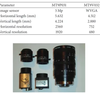
Table 3: Parameters of camera sensors.
Parameter MT9P031 MT9V032
Image sensor 5 Mp WVGA
Horizontal length (mm) 5.632 4.512
Vertical length (mm) 4.224 2.880
Horizontal resolution 2560 752
Vertical resolution 1920 480
Figure 4: Cameras and lenses used in VSN design.
3. Camera Models and Optics
The image sensors chosen to implement the monitoring nodes for sub VSNs in the above example include 5 Mp and WVGAs. The 5 Mp image sensor MT9P031 is used in camera model UI-5480CP-M from UEye and is shown in
Figure 4. The horizontal length𝑙ℎand the vertical length𝑙V of this sensor are 5.632 and 4.224 mm, respectively. Also, the horizontal resolution𝑟ℎand vertical resolution𝑟Vof this sensor are 2560 and 1920, respectively. These parameters are shown in Table 3. The power is applied to this camera module through Hirose connector while the data is received via Ethernet link.
The WVGA image sensor MT9V032 is used in camera model UI-1220SE-M from UEye and is shown inFigure 4. The horizontal length𝑙ℎand the vertical length𝑙Vof this sen-sor are 4.512 and 2.880 mm, respectively. Also, the horizontal resolution𝑟ℎand vertical resolution𝑟Vof this sensor are 752 and 480, respectively. These parameters are shown inTable 3. The camera is using a USB interface which is used to apply power as well as receive data from the camera module.
The cameras and the accompanied optics used to imple-ment the heterogeneous VSN are shown in Figure 4. The combination of a camera and the accompanied lens of relevant focal length form a monitoring node. An individual laptop machine is used with each monitoring node as data gathering and analysis platform. The 5 Mp camera module is connected to the laptop by using CAT 6 Ethernet cable. The power is supplied to the camera module by using 6 pin Hirose connector. The camera is connected to the laptop as client while the laptop is used as server. The WVGA camera is connected to the laptop by using a USB cable. The power to a camera node and laptop is supplied by using a 12 Volt rechargeable battery. A complete node is shown inFigure 5. The images of the bird are captured by UEye cockpit software.
Figure 5: A complete camera node.
This is the camera interface to capture images/videos or to change the controlling parameters of the camera.
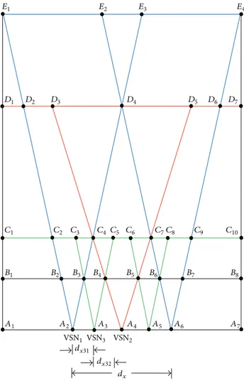
4. Coverage Model
The camera coverage model based on all the above design parameters is shown in Figure 6. The model contains five altitude lines𝐴, 𝐵, 𝐶, 𝐷, and 𝐸. The altitude line 𝐴 represents the ground plane and monitoring nodes are placed on this line. This line contains seven points from 𝐴1 to 𝐴7. The camera nodes of VSN1 are placed at points 𝐴2 and 𝐴6, the camera node of VSN2 is placed at point 𝐴4, and the camera nodes for VSN3 are placed at points 𝐴3 and 𝐴5. The second altitude line is 𝐵 which contains eight points from 𝐵1 to 𝐵8. The network VSN3 provides full coverage on this line by making intersections with VSN1and VSN2. The third altitude line is𝐶 which contains ten points from 𝐶1 to𝐶10. The VSN2 provides full coverage on this line by making intersections with VSN1. This altitude line also acts as the highest altitude boundary for VSN3. This is because the VSN3is not able to provide the required resolution above this altitude. The fourth altitude line is 𝐷 which contains seven points from𝐷1 to 𝐷7. This altitude line acts as the highest altitude boundary for VSN2. The VSN2is not able to provide the required resolution above this altitude. The last altitude line is𝐸 which contains four points from 𝐸1to𝐸4. This altitude line represents the highest altitude for VSN1as well as for the entire heterogeneous VSN, where an object can be monitored with the required minimum resolution.
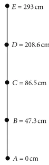
To perform coverage and resolution measurements, it is necessary to find the altitudes of the lines above ground and the distances of the points from the edge of the relevant lines. The altitude line𝐴 represents the ground so it has altitude 0 cm. The altitude line𝐵 is the lower altitude for VSN3; it is at the altitude 47.3 cm above the ground, as calculated before. The altitude line𝐶 is the higher altitude for VSN3or the lower altitude for VSN2. Thus, it is at altitude 86.5 cm above the ground. The altitude line𝐷 is the higher altitude for VSN2or the lower altitude for VSN1. Thus, it is at the altitude 208.6 cm above the ground. The altitude line𝐸 represents the higher altitude for VSN1. Thus, it is at the altitude 293 cm above the ground. All these altitudes are summarized inFigure 7.
After finding the altitudes of the lines, the distances of the points from the edge of the respective altitude lines are calculated. For altitude line𝐴, the distance of point 𝐴2from
A1 A2 A3 A4 A5 A6 A7 B1 B2 B3 B4 B5 B6 B7 B8 C1 C2 C3 C4 C5 C6 C7C8 C9 C10 D1 D2 D3 D4 D5 D6 D7 E1 E2 E3 E4 VSN1 VSN3 VSN2 dx dx32 dx31 Figure 6: VSN model.
point𝐴1can be calculated by solving the triangle𝐸1𝐴1𝐴2in
Figure 6. The distance of point𝐴2from point𝐴1is calculated and is found to be 68.8 cm. The distance between points𝐴2 and𝐴6is𝑑𝑥which is 97.9 cm. The distance of point𝐴6from point𝐴1is calculated by adding the distance of point𝐴1from 𝐴2and the distance of point𝐴2from𝐴6and is found to be 166.6 cm. The distance of point𝐴7from𝐴1is 235.4 cm. The point𝐴4is𝑑𝑥/2 distance away from𝐴2. Thus, the point𝐴4is at 117.7 cm away from𝐴1. The point𝐴3is at 22.19 cm distance from𝐴2, and point𝐴5is at 22.19 cm distance from𝐴6. Thus, the points𝐴3and𝐴5are at distances 91.0 and 144.5 cm away from𝐴1, respectively.
Similarly, the distances of the points on other altitude lines are calculated. For altitude line𝐵, the distances of the points𝐵2,𝐵3,𝐵4,𝐵5,𝐵6,𝐵7, and𝐵8from𝐵1 are 57.7, 79.9, 102.1, 133.3, 155.5, 177.7, and 235.4 cm, respectively. For altitude line𝐶, the distances of the points 𝐶2,𝐶3,𝐶4,𝐶5,𝐶6,𝐶7,𝐶8, 𝐶9, and𝐶10 from𝐶1 are 48.5, 70.7, 89.1, 111.3, 124.2, 146.3, 164.8, 186.9, and 235.4 cm, respectively. For altitude line𝐷, the distances of points𝐷2,𝐷3,𝐷4,𝐷5,𝐷6, and𝐷7from𝐷1 are 19.8, 48.6, 117.7, 186.8, 215.6, and 235.4 cm, respectively. For altitude line𝐸, the distances of the points 𝐸2,𝐸3, and𝐸4from
E = 293cm D = 208.6cm C = 86.5cm A = 0cm B = 47.3cm Figure 7: VSN altitudes.
Table 4: Values of the points in VSN model.
No. 𝐴 (cm) 𝐵 (cm) 𝐶 (cm) 𝐷 (cm) 𝐸 (cm) 1 0 0 0 0 0 2 68.8 57.7 48.5 19.8 97.9 3 91.0 79.9 70.7 48.6 137.5 4 117.7 102.1 89.1 117.7 235.4 5 144.5 133.3 111.3 186.8 — 6 166.6 155.5 124.2 215.6 — 7 235.4 177.7 146.3 235.4 — 8 — 235.4 164.8 — — 9 — — 186.9 — — 10 — — 235.4 — —
𝐸1are 97.9, 137.5, and 235.4 cm, respectively. The values of all these points are given inTable 4.
5. Measurements of VSN Parameters
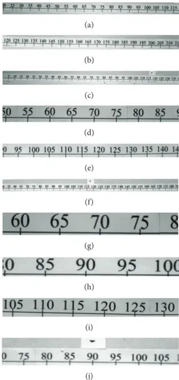
Two important parameters of a VSN which must be ensured are the full area coverage at a given lower altitude and the minimum required image resolution for an object, when moving at the given higher altitude. The remaining part of the paper describes the measurements to verify these parameters. The measurements are performed in a room. To measure all the distances, a 240 cm long scale is constructed on a long strip of paper. The markings on the scale are marked after every 5 cm. The scale is glued on a wall of the room. The wall is treated as sky for this experiment. A bird of size (1.08× 0.54) cm, shown inFigure 3, is printed on a card board and is used to measure the minimum required image resolution.
5.1. Coverage Measurements. This section measures coverage
at lower altitude of a given sub-VSN to verify whether this network is able to provide full coverage or not. The measurements are performed for altitudes 𝐷, 𝐶, and 𝐵, which are lower altitudes for the networks VSN1, VSN2, and VSN3, respectively. For coverage measurement, the images
are captured at the respective altitude line with the concerned camera nodes. The coverage of each node is measured and compared with the calculated coverage for that node to verify whether these nodes are covering the complete required area or there is some gap in the coverage.
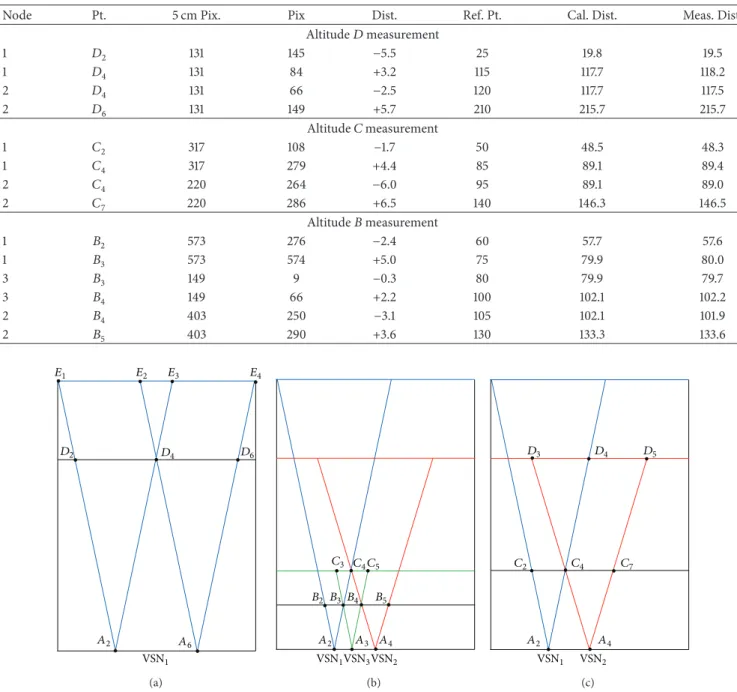
5.1.1. Altitude D. It is the lower altitude of VSN1, where full coverage of this network is assumed. For more clear visualiza-tion of this altitude, a separate model which is extracted from heterogeneous VSN model (Figure 6) is shown inFigure 8(a). To perform measurements for coverage verification at lower altitude of VSN1, the wall is treated as altitude line𝐷. The ground line 𝐴 of length 235.4 cm is drawn parallel to the wall, 208.6 cm away from the wall. The points𝐴2and𝐴6are marked at distances 68.8 cm and 166.6 cm from the edge of the line, according toFigure 8(a). Node 1 is placed at point 𝐴2while node 2 is placed at point𝐴6. Both nodes are using similar 5 Mp image sensors and lenses of focal length 12 mm, as discussed before. The complete setup is shown inFigure 9. The calculated distances expected to be covered by nodes 1 and 2 are from point𝐷2(19.8 cm) to𝐷4(117.7 cm) and from point𝐷4(117.7 cm) to𝐷6(215.6 cm). Images are captured with both monitoring nodes, and pixels are counted to measure the distances covered by these nodes.
The image captured by node 1 is shown inFigure 10(a). The pixel measurements in this figure show that about 131 pixels represent 5 cm distance. There are about 145 pixels from the left edge of the figure to the 25 cm point, which represents about 5.5 cm distance. Thus,𝐷2point has value of 19.5 cm. Similarly, there are about 84 pixels from right edge of the figure to the 115 cm point, which represent about 3.2 cm distance. Thus,𝐷4point has value of 118.2 cm.
The image captured by node 2 is shown inFigure 10(b). The pixel measurements in this figure show that about 131 pixels represent 5 cm distance. There are about 66 pixels from the left edge of the figure to the 120 cm point, which represents about 2.5 cm distance. Thus,𝐷4point has value of 117.5 cm. Similarly, there are about 146 pixels from the right edge of the figure to the 210 cm point, which represents about 5.6 cm distance. Thus,𝐷6point has value of 215.6 cm. All these values are shown inTable 5.
5.1.2. Altitude C. It is the lower altitude of VSN2, where full coverage of this network is assumed. For more clear visual-ization of this altitude, a separate model which is extracted from heterogeneous VSN model, is shown in Figure 8(b). To perform measurements for coverage verification at lower altitude of VSN2, the wall is treated as altitude line𝐶. The ground line𝐴 of length 235.4 cm is drawn parallel to the wall at a distance of 86.5 cm away from the wall. The points𝐴2 and𝐴4 are marked at distances 68.8 and 117.7 cm from the edge of the line, according toFigure 8(b). The camera node 1 is placed at point𝐴2while the camera node 2 is placed at point𝐴4. Both camera nodes 1 and 2 have similar 5 Mp image sensor, but different lens focal lengths, 12 mm and 8.5 mm, respectively. The calculated distances expected to be covered by nodes 1 and 2 are from point𝐶2(48.5 cm) to𝐶4(89.1 cm) and from point 𝐶4 (89.1 cm) to𝐶7 (146.3 cm). Images are
Table 5: Coverage measurements details.
Node Pt. 5 cm Pix. Pix Dist. Ref. Pt. Cal. Dist. Meas. Dist.
Altitude𝐷 measurement 1 𝐷2 131 145 −5.5 25 19.8 19.5 1 𝐷4 131 84 +3.2 115 117.7 118.2 2 𝐷4 131 66 −2.5 120 117.7 117.5 2 𝐷6 131 149 +5.7 210 215.7 215.7 Altitude𝐶 measurement 1 𝐶2 317 108 −1.7 50 48.5 48.3 1 𝐶4 317 279 +4.4 85 89.1 89.4 2 𝐶4 220 264 −6.0 95 89.1 89.0 2 𝐶7 220 286 +6.5 140 146.3 146.5 Altitude𝐵 measurement 1 𝐵2 573 276 −2.4 60 57.7 57.6 1 𝐵3 573 574 +5.0 75 79.9 80.0 3 𝐵3 149 9 −0.3 80 79.9 79.7 3 𝐵4 149 66 +2.2 100 102.1 102.2 2 𝐵4 403 250 −3.1 105 102.1 101.9 2 𝐵5 403 290 +3.6 130 133.3 133.6 A2 A6 D2 D4 D6 E1 E2 E3 E4 VSN1 (a) A2 A3 A4 B2 B3 B4 B5 C3 C4C5 VSN1VSN3VSN2 (b) A2 A4 C4 C7 C2 D4 D5 D3 VSN1 VSN2 (c)
Figure 8: VSN models, (a) VSN1, (b) VSN2, and (c) VSN3.
captured with both nodes, and pixels are counted to measure the distance covered by these nodes.
The image captured by node 1 is shown inFigure 10(d). The pixel measurements in this figure show that about 317 pixels represent 5 cm distance. There are about 108 pixels from the left edge of the figure to the 50 cm point, which represents about 1.7 cm distance. Thus,𝐶2 point has value of 48.3 cm. Similarly, there are about 279 pixels from the right edge of the figure to the 85 cm point, which represents about 4.4 cm distance. Thus,𝐶4point has value of 89.4 cm.
The image captured by node 2 is shown inFigure 10(e). The pixel measurements in this figure show that about 220 pixels represent 5 cm distance. There are about 264 pixels
from the left edge of the figure to the 95 cm point, which represents about 6.0 cm distance. Thus,𝐶4 point has value of 89.0 cm. Similarly, there are about 286 pixels from right edge of the figure to the 140 cm point, which represents about 6.5 cm distance. Thus, 𝐶7 point has value of 146.5 cm. All these values are given inTable 5.
5.1.3. Altitude B. It is the lower altitude of VSN3, where full coverage of this network is assumed. For more clear visual-ization of this altitude, a separate model which is extracted from heterogeneous VSN model is shown in Figure 8(c). To perform measurements for coverage verification at lower altitude of VSN3, the wall is treated as altitude line𝐵. The
Figure 9: VSN installation.
ground line𝐴 of length 235.4 cm is drawn parallel to the wall at a distance of 47.3 cm away from the wall. The points𝐴2,𝐴3, and𝐴4are marked at distances 68.8, 91.0, and 117.7 cm from the edge of the line, according toFigure 8(c). Camera node 1 is fixed at point𝐴2, camera node 2 is fixed at point𝐴4, while camera node 3 is fixed at point𝐴3. Both camera nodes 1 and 2 have similar 5 Mp image sensors but different lens focal lengths, 12 mm and 8.5 mm, respectively. Camera node 3 has WVGA camera sensor and lens of focal length 9.6 mm. The calculated distances expected to be covered by nodes 1, 3, and 2 are from point𝐵2(57.7 cm) to𝐵3(79.9 cm), from point𝐵3 (79.9 cm) to𝐵4(102.1 cm), and from point𝐵4(102.1 cm) to𝐵5 (133.3 cm), respectively.
The image captured by node 1 is shown inFigure 10(g). The pixel measurements in this figure show that about 573 pixels represent 5 cm distance. There are about 276 pixels from the left edge of the figure to the 60 cm point, which represents about 2.4 cm distance. Thus,𝐵2point has value of 57.6 cm. Similarly, there are about 574 pixels from the right edge of the figure to the 75 cm point, which represents about 5.0 cm distance. Thus,𝐵3point has value of 80.0 cm.
The image captured by node 3 is shown inFigure 10(h). The pixel measurements in this figure show that about 149 pixels represent 5 cm distance. There are about 9 pixels from the left edge of the figure to the 80 cm point, which represents about 0.3 cm distance. Thus,𝐵3 point has value of 79.7 cm. Similarly, there are about 66 pixels from the right edge of the figure to the 100 cm point, which represents about 2.2 cm distance. Thus,𝐵4point has value of 102.2 cm.
The image captured by node 2 is shown inFigure 10(i). The pixel measurements in this figure show that about 403 pixels represent 5 cm distance. There are about 250 pixels from the left edge of the figure to the 105 cm point, which represents about 3.1 cm distance. Thus, 𝐵4 point has value of 101.9 cm. Similarly, there are about 290 pixels from the right edge of the figure to the 130 cm point, which represents about 3.6 cm distance. Thus,𝐵5 point has value of 133.6 cm. All these values are given inTable 5.
5.2. Resolution Measurements. After measuring the coverage
at respective lower altitudes of the sub-VSNs, the mea-surement of the minimum achieved image resolution is performed for the given object, when moving at the higher altitude of the respective sub-VSN, to verify whether this resolution fulfills the minimum resolution criterion. The measurements are performed for altitudes𝐸, 𝐷, and 𝐶, which
(a) (b) (c) (d) (e) (f) (g) (h) (i) (j)
Figure 10: VSN measurements at different altitudes with different
nodes: (a–c) VSN1, altitude𝐷 node 1, altitude 𝐷 node 2, and altitude
𝐸, node 1; (d–f) VSN2, altitude𝐶 node 1, altitude 𝐶 node 2, and
altitude𝐷 node 1; (g–j) VSN3, altitude𝐵 node 1, altitude 𝐵 node 2,
altitude𝐵 node 3, altitude 𝐶 node 1.
are higher altitudes for the networks VSN1, VSN2, and VSN3, respectively. For resolution measurement, the images are captured at the respective altitude line with the concerned camera nodes. The resolution of the object image obtained by each node is measured for verification.
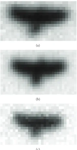
5.2.1. Altitude E. It is the higher altitude of VSN1(Figure 8(a)) where minimum required object image resolution is assumed. To perform measurements for resolution verification for VSN1, the wall is treated as altitude line 𝐸 and the bird image ofFigure 3 is fixed on the wall. The ground line𝐴 of length 235.4 cm is drawn parallel to the wall at a distance of 293 cm away from the wall. Both nodes 1 and 2 are placed the same way as for measuring the full coverage, and images are captured by these nodes. One such image captured by node 1 is shown inFigure 10(c). For more clear observation, a small portion ofFigure 10(c)which contains bird image is shown magnified inFigure 11(a). The bird pixels are measured along the width side by using segmentation.
(a)
(b)
(c)
Figure 11: Bird resolution at the highest altitude: (a) VSN1, (b) VSN2,
and (c) VSN3.
The number of pixels obtained is 19. This value is very near to the calculated value of 20.
5.2.2. Altitude D. It is the higher altitude of VSN2
(Figure 8(b)) where minimum required object image resolution is assumed. To perform measurements for resolution verification for VSN2, the wall is treated as altitude line𝐷. The ground line 𝐴 of length 235.4 cm is drawn parallel to the wall at a distance of 208.6 cm away from the wall. Both nodes 1 and 2 are placed the same way as for measuring the full coverage, and images are captured by these nodes. One such image captured by node 2 is shown inFigure 10(f). For more clear observation, a small portion ofFigure 10(f)which contains bird image is shown magnified in Figure 11(b). The bird pixels are measured along the width side by using segmentation. The number of pixels obtained is 19. This value is very near to the calculated value of 20.
5.2.3. Altitude C. It is the higher altitude of VSN3
(Figure 8(c)) where minimum required object image resolution is assumed. To perform measurements for resolution verification for VSN3, the wall is treated as altitude line𝐶. The ground line 𝐴 of length 235.4 cm is drawn parallel to the wall at a distance of 86.5 cm away from the wall. The
nodes 1, 3, and 2 are placed the same way as for measuring the full coverage, and images are captured by these nodes. One such image captured by node 3 is shown inFigure 10(j). For more clear observation, a small portion ofFigure 10(j)which contains bird image is shown magnified in Figure 11(c). The bird pixels are measured along the width side by using segmentation. The number of pixels obtained is 19. This value is very near to the calculated value of 20.
6. Results
The coverage measurement results inTable 5show that the measured values for different points are in accordance with the values calculated by heterogeneous VSN model. Even the measured values are broader than the calculated values. For example, the analysis of the range covered by node 1 at altitude line𝐷 between 𝐷2and𝐷4points (first two rows ofTable 5) shows that the calculated value of𝐷2 is 19.8 cm while the measured value is 19.5 cm. It shows that the node is providing coverage before the calculated value. Similarly, the calculated value of𝐷4is 117.7 cm while the measured value is 118.2 cm, which shows that the node is providing coverage after the calculated value. Thus, the node is providing reliable coverage of the required area. Similar is the case with other values in the table. Moreover, the resolution measurement results are also in accordance with the calculated values. The implementation cost comparison for both homogeneous and heterogeneous VSNs shows that the heterogeneous VSN provides more than 70% decrease in cost as compared to homogeneous VSN.
7. Conclusion
This paper discusses the design of a heterogeneous VSN for the surveillance of a volume between two altitude limits. Images are captured and measurements are performed to verify full coverage and minimum achieved resolution at lower and higher altitudes, respectively. The measurements verify that the heterogeneous VSN is able to provide full volume coverage between the given altitude limits. The core advantage of heterogeneous VSN over homogeneous VSN is the higher cost reduction.
References
[1] K. Obraczka, R. Manduchi, and J. Garcia-Luna-Aceves, “Man-aging the information flow in visual sensor networks,” in
Proceedings of the 5th International Symposium on Wireless Personal Multimedia Communication, 2002.
[2] H. Medeiros, J. Park, and A. Kak, “A light-weight event-driven protocol for sensor clustering in wireless camera networks,” in
Proceedings of the 1st ACM/IEEE International Conference on Distributed Smart Cameras (ICDSC ’07), pp. 203–210, Vienna,
Austria, September 2007.
[3] S. Soro and W. Heinzelman, “A survey of visual sensor net-works,” Advances in Multimedia, vol. 2009, Article ID 640386, 21 pages, 2009.
[4] Y. Charfi, N. Wakamiya, and M. Murata, “Challenging issues in visual sensor networks,” IEEE Wireless Communications, vol. 16, no. 2, pp. 44–49, 2009.
[5] M. Chitnis, Y. Liang, J. Y. Zheng, P. Pagano, and G. Lipari, “Wireless line sensor network for distributed visual surveil-lance,” in Proceedings of the 6th ACM International Symposium
on Performance Evaluation of Wireless Ad-Hoc, Sensor, and Ubiquitous Networks (PE-WASUN ’09), pp. 71–78, October 2009.
[6] Y.-C. Tseng, Y.-C. Wang, K.-Y. Cheng, and Y.-Y. Hsieh, “iMouse: an integrated mobile surveillance and wireless sensor system,”
Computer, vol. 40, no. 6, pp. 60–66, 2007.
[7] T. Brodsky, R. Cohen, E. Cohen-Solal et al., “Visual surveillance in retail stores and in the home,” in Advanced Video-Based
Surveillance Systems, pp. 50–61, Kluwer Academic, Boston,
Mass, USA, 2001.
[8] G. L. Foresti, C. Micheloni, L. Snidaro, P. Remagnino, and T. Ellis, “Active video-based surveillance system,” IEEE Signal
Processing Magazine, vol. 22, no. 2, pp. 25–37, 2005.
[9] P. Kulkarni, D. Ganesan, and P. Shenoy, “The case for multi-tier camera sensor networks,” in Proceedings of the 15th International
Workshop on Network and Operating Systems Support for Digital Audio and Video (NOSSDAV ’05), pp. 141–146, June 2005.
[10] D. Beymer, P. McLauchlan, B. Coifman, and J. Malik, “Real-time computer vision system for measuring traffic parameters,” in Proceedings of the IEEE Computer Society Conference on
Computer Vision and Pattern Recognition, pp. 495–501, June
1997.
[11] K. H. Lim, L. M. Ang, K. P. Seng, and S. W. Chin, “Lane-vehicle detection and tracking,” in Proceedings of the International Multi
Conference of Engineers and Computer Scientists, vol. 2, 2009.
[12] J. M. Ferryman, S. J. Maybank, and A. D. Worrall, “Visual surveillance for moving vehicles,” in Proceedings of the IEEE
Workshop on Visual Surveillance (ICCV ’98), pp. 73–80, 1998.
[13] D. Koller, J. Weber, and J. Malik, “Robust multiple car tracking with occlusion reasoning,” in Proceedings of the European
Conference on Computer Vision, pp. 189–196, 1994.
[14] D. Koller, J. Weber, T. Huang et al., “Towards robust automatic traffic scene analysis in real-time,” in Proceeding of International
Conference on Pattern Recognition, 1994.
[15] M. Xu, J. Orwell, L. Lowey, and D. Thride, “Architecture and algorithms for tracking football players with multiple cameras,”
Proceedings of IEE Vision, Image and Signal Processing, vol. 152,
no. 2, pp. 232–241, 2005.
[16] C. J. Needham and R. D. Boyle, “Tracking multiple sports players through occlusion, congestion and scale,” in Proceedings
of the British Machine Vision Conference, vol. 1, no. 2, pp. 93–102,
2001.
[17] R. Kays, S. Tilak, B. Kranstauber et al., “Camera traps as sensor networks for monitoring animal communities,” International
Journal of Research and Review in Wireless Sensor Networks, vol.
1, pp. 19–29, 2011.
[18] S. Uchiyama, H. Yamamoto, M. Yamamoto, K. Nakamura, and K. Yamazaki, “Sensor network for observation of seabirds in Awashima island,” in Proceedings of the International Conference
on Information Networking (ICOIN ’11), pp. 64–67, Barcelona,
Spain, January 2011.
[19] C. Micheloni, G. L. Foresti, and L. Snidaro, “A co-operative multi camera system for video-surveillance of parking lots,” in Proceedings of the IEE Workshop on Intelligent Distributed
Surveillance Systems, pp. 21–24, 2003.
[20] J. Campbell, P. B. Gibbons, and S. Nath, “Irisnet: an internet-scale architecture for multimedia sensors,” in Proceedings of the
ACM Multimedia, 2005.
[21] J. Krumm, S. Harris, B. Meyers, B. Brumit, M. Hale, and S. Shafer, “Multi-camera multi-person tracking for easy living,” in
Proceedings of the 3rd IEEE International Workshop on Visual Surveillance, pp. 3–10, 2000.
[22] J. Wang and B. Yan, “A framework of heterogeneous real-time video surveillance network management system,” in Proceedings
of the International Conference on Information Technology, Computer Engineering and Management Sciences (ICM ’11), pp.
218–221, Nanjing, China, September 2011.
[23] P. Kulkarni, D. Ganesan, and P. Shenoy, “The case for multi-tier camera sensor networks,” in Proceedings of the 15th International
Workshop on Network and Operating Systems Support for Digital Audio and Video (NOSSDAV ’05), pp. 141–146, June 2005.
[24] H. Aghajan and A. Cavallaro, Multi-Camera Networks,
Princi-ples and Applications, Academic Press, 2009.
[25] E. H¨orster and R. Lienhart, “Approximating optimal visual sensor placement,” in Proceedings of the IEEE International
Conference on Multimedia and Expo (ICME ’06), pp. 1257–1260,
Toronto, Canada, July 2006.
[26] E. H¨orster and R. Lienhart, “On the optimal placement of mul-tiple visual sensors,” in Proceedings of the 4th ACM International
Workshop on Video Surveillance and Sensor Networks, 2006.
[27] N. Ahmad, N. Lawal, M. O’Nils, B. Oelmann, M. Imran, and K. Khursheed, “Model and placement optimization of a sky surveillance visual sensor network,” in Proceedings of
the 6th International Conference on Broadband and Wireless Computing, Communication and Applications (BWCCA ’11), pp.
Submit your manuscripts at
http://www.hindawi.com
Control Science and Engineering
Journal of
Hindawi Publishing Corporation
http://www.hindawi.com Volume 2013
Machinery
Hindawi Publishing Corporation
http://www.hindawi.com Volume 2013Part I
Hindawi Publishing Corporation
http://www.hindawi.com Volume 2013
Distributed
Sensor Networks
International Journal of ISRN Signal ProcessingHindawi Publishing Corporation
http://www.hindawi.com Volume 2013
Hindawi Publishing Corporation
http://www.hindawi.com Volume 2013 Mechanical Engineering Advances in Modelling & Simulation in Engineering
Hindawi Publishing Corporation
http://www.hindawi.com Volume 2013
Advances in OptoElectronics
Hindawi Publishing Corporation
http://www.hindawi.com Volume 2013
ISRN
Sensor Networks
Hindawi Publishing Corporation
http://www.hindawi.com Volume 2013
VLSI Design
Hindawi Publishing Corporation
http://www.hindawi.com Volume 2013
Hindawi Publishing Corporation
http://www.hindawi.com Volume 2013
Hindawi Publishing Corporation
http://www.hindawi.com Volume 2013
The Scientific
World Journal
ISRN
Robotics
Hindawi Publishing Corporation
http://www.hindawi.com Volume 2013
International Journal of
Antennas and
Propagation
Hindawi Publishing Corporation
http://www.hindawi.com Volume 2013
ISRN
Electronics
Hindawi Publishing Corporation
http://www.hindawi.com Volume 2013
Hindawi Publishing Corporation
http://www.hindawi.com Volume 2013 Journal of
Sensors
Hindawi Publishing Corporation
http://www.hindawi.com Volume 2013
Electronic Components
Chemical Engineering
International Journal of
Hindawi Publishing Corporation
http://www.hindawi.com Volume 2013 Hindawi Publishing Corporation
http://www.hindawi.com Volume 2013 Electrical and Computer Engineering
Journal of
ISRN
Civil Engineering
Hindawi Publishing Corporation
http://www.hindawi.com Volume 2013
Advances in
Acoustics &
Vibration
Hindawi Publishing Corporation