Department of Wildlife, Fish, and Environmental Studies
An investigation into whether poaching
creates an ecological trap for white
rhinoceros in Hluhluwe-iMfolozi Park, South
Africa
En undersökning för att reda ut om tjuvskytte orsakar en
ekologisk fälla för vita noshörningar i Hluhluwe-iMfolozi Parken,
Sydafrika
An investigation into whether poaching creates an ecological
trap for white rhinoceros in Hluhluwe-iMfolozi Park, South Africa
En undersökning för att reda ut om tjuvskytte orsakar en ekologisk fälla för vitanoshörningar i Hluhluwe-iMfolozi Parken, Sydafrika
Alice Michel
Supervisor: Joris Cromsigt, Swedish University of Agricultural Sciences, Department of Wildlife, Fish, and Environmental Studies
Assistant supervisor: Elizabeth le Roux, Nelson Mandela University, Department of Zoology Examiner: Navinder Singh, Swedish University of Agricultural Sciences, Department
of Wildlife, Fish, and Environmental Studies
Credits: 30 credits
Level: Second cycle, A2E
Course title: Master degree thesis in Biology at the Department of Wildlife, Fish, and Environmental Studies
Course code: EX0633
Course coordinating department: Department of Wildlife, Fish, and Environmental Studies
Place of publication: Umeå
Year of publication: 2019
Cover picture: Alice Michel
Title of series: Examensarbete/Master's thesis
Part number: 2019:8
Online publication: https://stud.epsilon.slu.se
Keywords: ecological trap, rhinoceros, maladaptation, megaherbivore,
In an ecological trap, animals choose habitat based upon cues that once led mem-bers of their species to optimal habitat, but now lead to habitat where individual fitness is reduced because of changing conditions. The southern white rhinoceros (Ceratotherium simum) is a threatened species due to poaching for its keratin horn. Here, I investigate the degree to which poaching creates an ecological trap for white rhinoceros in South Africa’s Hluhluwe-iMfolozi Park. To this end, I develop a model for white rhino habitat preference and analyse rhino movement through time over the gradient of habitat preference and poaching risk. Three aspects of the eco-logical trap scenario were assessed: environmental habitat quality in hotspots rela-tive to cold-spots for poaching, rhino movement into high-quality habitat regardless of poaching risk, and the impact of poaching on white rhino fitness at the popula-tion level. I found that while high quality habitat exists in poaching hotspots, net colonization was higher into high quality habitat in low-risk areas for poaching than in high-risk poaching hotspots. Further, fitness has declined for rhino populations in hotspots relative to cold-spots of the same quality, and likely represents a loss in fitness to the park population as a whole. While at this time there is little evidence to suggest rhino are pulled away from high quality cold-spots to areas at high risk for poaching, continued monitoring of the habitat quality-risk gradient is crucial to understanding and managing the white rhino population in Hluhluwe-iMfolozi Park.
Keywords: ecological trap, rhinoceros, maladaptation, megaherbivore, source-sink, habitat quality, middens
1 Introduction 5
2 Materials & Methods 9
2.1 Study Site 9
2.2 Data Collection 11
2.2.1 Mapping poaching hotspots 11
2.2.2 Midden density and associated habitat variables along transects 12 2.2.3 Mapping grazing lawn cover prior to rhino poaching 15 2.2.4 Rhino density measured along aerial transects 15
2.3 Analyses 17
2.3.1 Middens as a proxy for rhino density 17
2.3.2 Assessing white rhino habitat preference in HiP 17 2.3.3 Assessing habitat quality of poaching hotspots in HiP 18 2.3.4 Assessing rhino movement into poaching hotspots 18
2.3.4.1
Midden freshness 19
2.3.4.2
White rhino population demography 19
3 Results 21
3.1 Data Collection 21
3.1.1 Road transects 21
3.1.2 Grazing lawn maps 22
3.2 Analyses 22
3.2.1 Middens as a proxy for rhino density 22
3.2.2 Assessing white rhino habitat preference in HiP 24 3.2.3 Assessing habitat quality of poaching hotspots in HiP 25 3.2.4 Assessing rhino movement into poaching hotspots 27
3.2.4.1
Midden freshness 27
3.2.4.2
White rhino population demography 27
4 Discussion 33
4.1 Fitness and resource quality mismatch in hotspots 33
4.2 Rhino preference for high-quality cold-spots 35
4.3 Severity of the potential trap 37
4.4 Future directions 37
4.5 Conclusions 39
References 41
Acknowledgements 47
Evolution has generated a staggering degree of biodiversity, each species having, over time, accumulated mutations that enabled adaptation to their surroundings. Nevertheless, when surroundings rapidly change, there is no guarantee that a pre-viously well-adapted animal will continue to thrive. Fast-paced environmental change is on the rise, due to the activities of our own species. As a result, many species are now at risk of expressing maladaptive traits, or traits that have negative fitness consequences (Crespi 2000). When an adaptive behaviour becomes mala-daptive, and individuals do not change their behaviour, it is considered an evolu-tionary trap (Robertson, Rehage & Sih 2013). Evoluevolu-tionary traps pertain to food, mate, and habitat choice; an evolutionary trap in habitat-selection is also called an ecological trap (Robertson & Hutto 2006).
In an ecological trap scenario, an animal chooses to settle in habitat where it does poorly relative to other available habitats because the cues it uses to determine habitat quality have become decoupled from realized habitat quality (Battin 2004; Robertson & Hutto 2006; Hale & Swearer 2016). For an ecological trap to arise, fitness must differ between habitats, individuals must prefer higher-fitness areas, and then fitness must be lowered in the preferred habitat relative to less-preferred habitats, but individuals must still either prefer this habitat as much (‘equal-preference trap’) or more (‘severe trap’) than others (Robertson & Hutto 2006). Common examples include sea turtle hatchlings moving towards city lights instead of the beach (Witherington 1992), insects attracted to solar panels instead of water (Horváth et al. 2010), and birds nesting in human-altered environments (Robertson & Hutto 2006; Demeyrier et al. 2016; Hale & Swearer 2016). Ecological traps have typically been most rigorously documented in insects and birds (Robertson, Rehage & Sih 2013), and seldom in mammals, though there are examples in leop-ards and wild dogs living in reserves in southern Africa (Balme, Slotow & Hunter 2010; van der Meer et al. 2014). These carnivores are drawn to the edges of re-serves due to higher prey abundance, lower intraspecific competition, and/or to
avoid lions, but fall into an ecological trap because of human encounters and death at the reserve edge (Balme, Slotow & Hunter 2010; van der Meer et al. 2014). Another species faced with rapid environmental change is the white rhinoceros (Ceratotherium simum). As a 2,000-kg megaherbivore, rhino are considered to be relatively invulnerable to predation (Owen-Smith 1988), and while people were likely hunting rhino from early on (Churchill 1993), advances in weaponry rapidly increased the risk of human predation on rhino over the past two centuries. In the early 20th century, the southern white rhinoceros was extirpated from most of its ancestral range, but it has since undergone a population rebound thanks to the creation of game reserves, especially Hluhluwe-iMfolozi Park (HiP), in KwaZulu-Natal, South Africa (Rookmaaker 2000). Within HiP, rhino have been protected for 124 years (Cromsigt, Archibald & Owen-Smith 2017). However, rhino are now again threatened by poaching for their keratin horn (Thomas 2010; Emslie & Knight 2014; Ferreira et al. 2017; Dang Vu & Nielsen 2018). In HiP, rhino poach-ing occurs in specific regions of the park, whether due to accessibility or high rhi-no density, or some combination of the two. This creates areas of high poaching risk and areas of relatively low risk, and presents an opportunity to determine if poaching acts as an ecological trap for white rhino by potentially drawing them into areas of the park that are of good resource quality but high-risk for poaching. Such a trap would occur if high-intensity poaching occurs in high quality habitat in terms of resources that continues to be highly attractive to rhino, and thus, mala-daptively, draws rhino into the trap habitat despite the novel poaching risk (Figure 1). Previous work has shown rhino prefer savannah grassland, riverine, and wood-land systems, with low slope and water holes (Owen-Smith 1988; Shrader, Owen‐ Smith & Ogutu 2006). During the wet season and periods during the dry season with rainfall, rhino rely most strongly on areas with short-grassland grazing lawns, which they maintain through their high-intensity grazing (Waldram, Bond & Stock 2008). During the dry season, they tend to loosen their requirements, shifting to the utilization of shade grasses like Panicum maximum and as the season progress-es to medium-tall Themeda grasslands, while maintaining the same general diet preference and food intake throughout the year (Owen-Smith 1988; Shrader, Ow-en‐Smith & Ogutu 2006).
An ecological trap is an extension of the classic source-sink model (Pulliam 1988), whereby “source” habitats are high quality in terms of resources yet low poaching risk. When they reach carrying capacity, quality is diminished through competi-tion, causing dispersing animals to seek out alternative habitats. Pre-threat, the only option would be to move into lower-quality habitat, where population growth
is slower than the source due to environmental limitations. This describes a tradi-tional low-quality “sink” habitat in ecological theory (Pulliam 1988). But, if there is high-quality habitat that is not at carrying capacity due to poaching, rhinos may follow their previously adaptive behavioural response to habitat cues and choose to move there in spite of the novel poaching risk. This habitat then becomes a high-quality “sink”. Poachers temporarily drain the sink, yet more dispersers steadily move in.
Here, I hypothesized that:
1.) White rhino prefer habitat that includes both short and medium-tall grass-lands for feeding, woodland for shade when resting, low slope, and access to water.
2.) Good-quality habitat that meets the criteria in (1) is present in areas at high risk to poaching.
3.) Rhino will move into these good-quality, yet high poaching areas in (2), making the rate of immigration higher into the trap habitat than into the source and sink habitats (Figure 1). Since sub-adult rhinos are the dispers-er age-category within the white rhino population (Shraddispers-er & Owen-Smith 2002), this movement into poaching hotspots would also manifest in pro-portionally more sub-adult rhinos into the high-quality, high-risk areas in (2) after the onslaught of poaching began, relative to that in high quality, low-risk areas and relative to before poaching intensified.
If these hypotheses hold, it would suggest that poaching creates an ecological trap for white rhino.
Figure 1. Depiction of the hypothesized ecological trap scenario for white rhino in
HiP. According to ecological theory, in the natural system animals will utilize the full potential of high-quality areas and growth rate will be maximized (λ > 1; top left quadrat), until the carrying capacity in these areas is reached. At this time, disperser individuals, such as sub-adults, will leave these “source” habitats and move into lower-quality “sink” habitat, where the growth rate is low (λ < 1) (Pulliam 1988) (bottom row). In the upper right quadrat, habitat quality in terms of resource availability is high, but realized habitat quality has recently become low due to poaching. If rhinos leaving the source habitat choose to move into the next highest-quality habitat in terms of resource quality (thick arrow), they suffer re-duced fitness due to poaching and the high-quality area functions as a sink; an ecological trap occurs (Battin 2004). Alternatively, if rhino habitat selection is not only based on resource quality, individuals may avoid the risk and move to the low quality safe areas (thin arrow). In low quality sink areas where poaching occurs despite potentially lower numbers of rhino, rhino are not expected to return at the same rates as in high-quality high-risk areas (lower right quadrat). Figure adapted from Battin, 2004.
2.1 Study Site
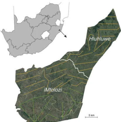
This study was conducted in Hluhluwe-iMfolozi Park, a 90,000 ha fenced reserve in KwaZulu-Natal, South Africa (Cromsigt, Archibald & Owen-Smith 2017). HiP includes a diverse range of habitat types within the southern African savannah biome, including open grassland, thicket, and woodland (Whateley & Porter 1983), due to variation in geology, soil, topology, rainfall, fire, and herbivory across the park (Archibald et al. 2005; Cromsigt & Olff 2008; Veldhuis et al. 2017). HiP includes two regions: northern Hluhluwe Park and southern iMfolozi Park, which are divided by an open-access corridor road (Figure 2). Hluhluwe is more mountainous and is characterized by mesic savannah, while iMfolozi is drier and flatter, with undulating hills and semi-arid savannah vegetation.
What is today HiP was once the only place in Africa where the southern white rhinoceros was not completely extirpated due to hunting; even there, the white rhino population was hunted down to an estimated 200 individuals by 1900 (Rookmaaker 2000). Today, HiP has a high density of white rhino, and all south-ern white rhino elsewhere are descended from HiP stock (Cromsigt, Archibald & Owen-Smith 2017). Since 1961, park management have translocated approximate-ly 10,000 rhino from HiP, a process that has repopulated the southern white rhino across southern Africa (Player 1967; Rookmaaker & Antoine 2012; Cromsigt, Archibald & Owen-Smith 2017). Moreover, HiP is one of the only places where they reach ecologically functional, and likely historically representative, densities, with their grazing driving lawn formation and ecological cascades (Rookmaaker 2000; Cromsigt, Archibald & Owen-Smith 2017; le Roux, Kerley & Cromsigt 2018).
Currently however, the threat against rhino is renewed, with poaching posing the greatest threat to rhinos worldwide (Ripple et al. 2015). In HiP, poaching has in-creased dramatically in recent years, starting in 2007 with the rise in poaching across southern Africa (Thomas 2010) and increasing since then in HiP. Poaching
statistics for HiP are confidential, but across South Africa 769 rhino were poached in 2018 (Thomas 2019).
The habitat heterogeneity, high rhino density, and spatial heterogeneity in poach-ing intensity across the park made Hluhluwe-iMfolozi Park the ideal location to test the ecological trap hypothesis for white rhino. Furthermore, HiP management, Ezemvelo KZN Wildlife, has kept a database of rhino density and removals through time that made this project possible.
Figure 2. Map of the study site, Hluhluwe-iMfolozi Park in KZN, South Africa,
showing the dividing corridor road in white between the two regions and the 34 fixed-line walking transects from which grazing lawn data from 2004 (brown lines) and 2014 (brown lines and green lines) was obtained.
Due to the crisis whose impact this project aimed to study, rhino density and re-movals data is sensitive information. Permission to use this data was granted under project registration number E/5141/02. Hence maps of rhino density and removals are not shown for security reasons.
2.2 Data Collection
2.2.1 Mapping poaching hotspots
In order to study rhino movement with regard to the poaching risk gradient, I de-fined high-risk, “hotspot” areas for poaching and low-risk, “cold-spot” areas. HiP management have recorded GPS locations for individual rhino poached from late 2011 to the present based on carcasses found and for legal live rhino removals by management for translocations to other reserves from 2000 through 2016, when translocations stopped.
I considered the size of male rhino territories in HiP, 1.65 km2 (Owen-Smith
1975), as the maximum area of impact of a poaching event, and hence any area
within 724 m (the radius of a circle of area 1.65 km2) of a poached rhino was
con-sidered as falling within a hotspot. While females and non-territorial males are not constrained to this range size, it is also roughly consistent with average mesoher-bivore flight distance (Tarakini et al. 2014). Thus, the coordinates of each poach-ing event in park records were buffered by radius 724 m in QGIS 3.4.3 (QGIS Development Team 2018), giving a circle around every poached animal of area
1.65 km2. The circles for every poaching event were merged, resulting in a
poach-ing hotspot map. The same method was used to define management removal areas based on the HiP management removals database. It was important to identify areas of impact of poaching removals and of management removals for evaluating rhino habitat preference (hypothesis 1; see below for detailed methods).
I made a grid of sizes 3, 12, and 25 km2 over HiP and calculated the proportion of
each cell that was encompassed by a poaching hotspot or area affected by man-agement removal by overlaying the hotspot maps described above over the grid cells. These grid sizes were chosen to represent the maximum male rhino range
(2.6 km2), average female rhino home range (11.6 km2), and maximum female
rhino annual range (21 km2) in HiP (Owen-Smith 1988). Cells with less than 10%
poaching hotspot and management removal area were considered cold-spots, which were used to determine which habitat rhino prefer (hypothesis 1). Cells with at least 50% cover by poaching hotspot were considered hotspots for poaching and were used to assess habitat quality and migration into poaching hotspots relative to cold-spots for poaching only (not management removals) (hypotheses 2&3). The intermediate range of the poaching gradient was excluded to avoid ambiguity. The number of removals per year was also calculated per grid cell, using ‘rgeos’ and ‘maptools’ in R to get an estimate of removal intensity (Bivand & Lewin-Koh 2013; Bivand et al. 2018; R Core Team 2019).
2.2.2 Midden density and associated habitat variables along road transects
To quantify rhino habitat preference across HiP, I relied on midden density as a proxy for rhino density. Rhino deposit dung in communal latrines, or middens, which also function as sites of social interaction (Marneweck, Jürgens & Shrader 2018). Each territorial male has many middens within his territory that all rhino passing through use (Owen-Smith 1975). Midden distribution is likely representa-tive of long-term rhino distribution, while dung freshness shows whether there has been recent local rhino activity (Marneweck et al., 2018; Ezemvelo KZN Wildlife Staff, personal communication).
To measure midden density across HiP, I drove 216 km of road transects and rec-orded midden presence and freshness for all middens observed within 20m of the road in October 2018. Road transects were undertaken by driving at 10 km/h along tourist roads and management tracks covering all main areas of the park. Two observers and a driver were present in the vehicle, a Ford Ranger, and each ob-server recorded middens on either the left or right side of the road. A total of 106 km of transect ran through poaching hotspots, 26 km ran through just management removal hotspots, and 82 km were in cold-spots. Midden freshness was catego-rized as “recent”, or within about two weeks of age (moist interior), or “old”, dry and older than two weeks old. A 75 km subset of roads was driven twice (2-4 weeks apart) to check the precision of dung freshness estimates. A range finder was used to measure the distance to each midden.
Along these same transects I also mapped variables that are likely to be important in terms of rhino habitat quality (Shrader, Owen‐Smith & Ogutu 2006). These variables included: grazing lawn coverage, 2018 burn extent, and habitat type. Grazing lawns are communities of stoloniferously growing grass both eaten and maintained by rhino through their high-intensity, low-specificity feeding (Waldram, Bond & Stock 2008). Burns were considered important because fresh growth attracts a number of different grazer species (Archibald et al. 2005). In 2018, fires occurred in September and early October. Lawns and burns were mapped separately on each side of the road by marking a GPS location of each 10x10m lawn or burnt patch for smaller patches, or by marking the start and end point while driving along the road for longer lawns and burn patches. Only patches within 15m of the road of size at least 10x10m were marked. The left and right cover was averaged for analyses. Habitat type was defined as “open” or “closed”. Open habitat included grassland, Acacia- and Dichrostachys-encroached grass-land, and open woodgrass-land, while closed habitat refers to forest, closed woodland (tree canopies touching), and riverine habitats. I also recorded road type, as asphalt or dirt, whenever driving into a different type. I hypothesized that rhino prefer to walk along dirt roads, and hence midden usage may be biased. GPS points and notes were recorded using the Gaia GPS application on an iPhone 5S.
I used QGIS 3.4.3 (QGIS Development Team 2018) and ‘rgeos’ and ‘maptools’ in R (Bivand & Lewin-Koh 2013; Bivand et al. 2018; R Core Team 2019) to map coordinates for middens, grazing lawns, burn scars, habitat type, road type, and the
total driving path into the same grid cells of sizes 3, 12, and 25 km2 as described
before. Midden density and lawn and burn cover were calculated as the count of middens per km of road driven in each grid cell and the summed length of lawn or burn patches recorded per km road.
To augment on-the-ground measurements, I mapped river cover, topography, woody cover, and fire frequency from satellite imagery and rainfall from long-term datasets maintained by park management. River cover was the total length of waterways per square kilometre. Topography was quantified from a 90m resolu-tion DEM (Jarvis et al. 2008) as mean slope per grid cell. Woody cover was in-tended as a more quantitative measure of habitat type. It was the fraction of woody biomass per grid cell extracted from a 0.5 m resolution map of woody cover creat-ed using Google Earth images (Veldhuis et al. 2017). Woody cover rangcreat-ed from 10% to 60% per grid cell and the median, 23.6%, was considered the cut-off be-tween open and closed habitat type since it reflected our on-the-ground habitat type measure. Since rainfall varies spatially across HiP, I used a 250m resolution elevation-weighted interpolation map of rainfall based on records at 17 rainfall stations across HiP from 2001-2007 (le Roux et al. 2019) and calculated the aver-age rainfall over this time period per grid cell. This was used as an estimate of relative rainfall index per grid cell across the park for 2018. Fire frequency was measured as the number of years from 2002 to 2016 during which at least 25% of grid cell area burned. Annual burn maps from this period were provided by T. Herkenrath (unpublished MSc thesis in prep) and constructed based on park rec-orded burn maps and MODIS satellite imagery (Giglio et al. 2018). All habitat variables measured are summarized in Table 1.
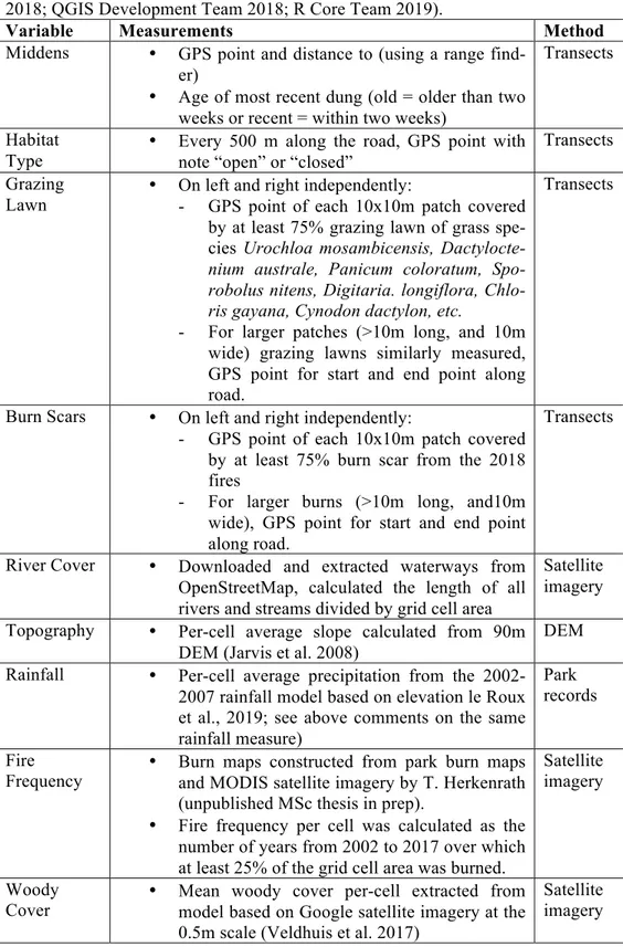
Table 1. Midden and habitat variable measurements. Calculations and processing
of data was done in QGIS 3.4.3 and R (Bivand & Lewin-Koh 2013; Bivand et al. 2018; QGIS Development Team 2018; R Core Team 2019).
Variable Measurements Method
Middens • GPS point and distance to (using a range
find-er)
• Age of most recent dung (old = older than two weeks or recent = within two weeks)
Transects
Habitat
Type • Every 500 m along the road, GPS point with note “open” or “closed”
Transects Grazing
Lawn • On left and right independently: - GPS point of each 10x10m patch covered
by at least 75% grazing lawn of grass spe-cies Urochloa mosambicensis,
Dactylocte-nium australe, Panicum coloratum, Spo-robolus nitens, Digitaria. longiflora, Chlo-ris gayana, Cynodon dactylon, etc.
- For larger patches (>10m long, and 10m wide) grazing lawns similarly measured, GPS point for start and end point along road.
Transects
Burn Scars • On left and right independently:
- GPS point of each 10x10m patch covered by at least 75% burn scar from the 2018 fires
- For larger burns (>10m long, and10m wide), GPS point for start and end point along road.
Transects
River Cover • Downloaded and extracted waterways from
OpenStreetMap, calculated the length of all rivers and streams divided by grid cell area
Satellite imagery
Topography • Per-cell average slope calculated from 90m
DEM (Jarvis et al. 2008)
DEM
Rainfall • Per-cell average precipitation from the
2002-2007 rainfall model based on elevation le Roux et al., 2019; see above comments on the same rainfall measure)
Park records
Fire
Frequency • Burn maps constructed from park burn maps and MODIS satellite imagery by T. Herkenrath (unpublished MSc thesis in prep).
• Fire frequency per cell was calculated as the number of years from 2002 to 2017 over which at least 25% of the grid cell area was burned.
Satellite imagery
Woody
Cover • Mean woody cover per-cell extracted from model based on Google satellite imagery at the
0.5m scale (Veldhuis et al. 2017)
Satellite imagery
2.2.3 Mapping grazing lawn cover prior to rhino poaching
Since rhino maintain grazing lawns, lawn cover in hotspots may be lower in 2018 relative to before rhino removals. Grazing lawns can be recreated if rhino return, but only in areas that have the capacity to support them. Soil, geology, drainage, and grass species can predispose an area to supporting the grazing lawn ecotype if rhino maintain it (Cromsigt & Olff 2008; Hempson et al. 2015). Since I was inter-ested in habitat quality before rhino removals, I built a map of lawn cover across HiP from vegetation surveys on fixed-line transects undertaken in 2004 and 2014 (le Roux 2018). Lawn cover was recorded on 26 of 32 transects (covering a dis-tance of 191.9 km in Hluhluwe and the northern half of iMfolozi; Figure 2) during 2004 and on all 32 transects (covering a distance of 278.6 km over the entire park) during 2014. On the fixed-line transects, an observer recorded lawn as present or absent in each 5m stretch along the transect (Cromsigt, Prins & Olff 2009; le Roux 2018). To mark a 5 m stretch as covered by grazing lawn, lawn species had to cover at least 75% of a 5 x 10 m patch (5m along the transect and 5 m to both sides of the transect). I estimated lawn cover per grid cell by summing the number of 5 x 10 m lawn patches in each grid cell, and dividing by the total number of 5 x 10 m patches surveyed in each grid cell.
I used linear regression to first determine how well lawn cover in 2004 predicted lawn cover in 2014 (using only grid cells monitored in both 2004 and 2014) and, second, to check how well 2014 lawn cover predicted lawn cover measured along road transects in 2018. I performed the latter regression separately for poaching hotspots and for cold-spots.
2.2.4 Rhino density measured along aerial transects
To measure white rhino distribution through time, I estimated rhino density from aerial census data collected on an annual basis by Ezemvelo KZN Wildlife man-agement in iMfolozi Park (the northern Hluhluwe section is not surveyed). Every dry season (roughly in September every year) since 2008, park management has conducted a survey from a fixed-wing airplane counting all the white rhino along complete-coverage aerial transects over the southern iMfolozi region of HiP. They record a GPS location for every rhino sighting and note the age category of each individual. Age is given in the following classes: A is a calf less than 3 months, B is a calf 3-12 months, C is 1-2 years, D is 2-3.5 years, E is 3.5-7 years, and F ani-mals are sexually mature (Emslie, Adcock & Hansen 1995).
I used the census data to calculate a number of population metrics per grid cell (Table 2). For all three grid sizes, I calculated annual rhino density and propor-tional rhino density averaged between 2008 and 2018. For the three other metrics
(see table 2), I used the 12 km2 grid cell size only. I used R to subset the grid cells
to just the iMfolozi region, then counted the number of rhino by age class in each grid cell (Bivand & Lewin-Koh 2013; Bivand et al. 2018; R Core Team 2019).
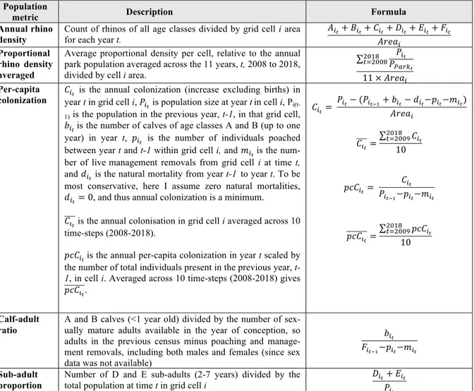
Table 2. White rhino population metrics, calculated per grid cell based off of
an-nual aerial counts of individual rhino of age classes A, B, C, D, E, and F through time.
Population
metric Description Formula
Annual rhino density
Count of rhinos of all age classes divided by grid cell i area for each year t.
!!!+ !!!+ !!!+ !!!+ !!!+ !!!
!"#$! Proportional
rhino density averaged
Average proportional density per cell, relative to the annual park population averaged across the 11 years, t, 2008 to 2018, divided by cell i area.
!!! !!"#$! !"#$ !!!""# 11 × !"#$! Per-capita
colonization !year t in grid cell i, !!! is the annual colonization (increase excluding births) in !! is population size at year tin cell i, P
i(t-1) is the population in the previous year, t-1, in that grid cell, !!!is the number of calves of age classes A and B (up to one
year) in year t, !!! is the number of individuals poached
between year t and t-1 within grid cell i, and !!! is the
num-ber of livemanagement removals from grid cell i at time t, and !!! is the natural mortality from year t-1 to year t. To be
most conservative, here I assume zero natural mortalities, !!!= 0, and thus annual colonization is a minimum.
!!! is the annual colonisation in grid cell i averaged across 10
time-steps (2008-2018).
!"#!!is the annual per-capita colonization in year t scaled by
the number of total individuals present in the previous year,
t-1, in cell i. Averaged across 10 time-steps (2008-2018) gives
!"#!!. !!!= !!!− (!!!!!+ !!!− !!!−!!!−!!!) !"#$! !!!= !!! !"#$ !!!""# 10 !"#!! = !!! !!!!!−!!!−!!! !"#!!= !"#!! !"#$ !!!""# 10 Calf-adult ratio
A and B calves (<1 year old) divided by the number of sex-ually mature adults available in the year of conception, so adults in the previous census minus poaching and manage-ment removals, including both males and females (since sex data was not available)
!!!
!!!!!−!!!−!!!
Sub-adult proportion
Number of D and E sub-adults (2-7 years) divided by the total population at time t in grid cell i
!!!+ !!!
2.3 Analyses
To test whether poaching acts as an ecological trap to white rhino I evaluated: a) Whether middens can be used as a proxy for rhino density;
b) Which criteria defines good quality habitat for rhino, based on midden density;
c) Whether poaching hotspots contain good quality habitat; and d) Whether rhino move into hotspots following poaching events.
2.3.1 Middens as a proxy for rhino density
The suitability of middens along road transects as a proxy for rhino density was investigated using white rhino aerial census. I modelled all middens as well as only middens that contained fresh dung as a function of rhino density using a qua-si-Poisson model offset by road length, separately for the three grid cell sizes: 12
km2, 3 km2 and 25 km2. I used only grid cells containing at least 1 km of road.
Quasi-poisson was chosen over Poisson because the overdispersion parameter exceeded 1.5 (Zuur et al. 2009). All model residuals were visually inspected for normality, heteroskedasticity, and violation of independence.
2.3.2 Assessing white rhino habitat preference in HiP
The density of recently used middens was used to determine which habitat
varia-bles contribute to rhino habitat preference at the 12 km2 grid cell size. To avoid
rhino removal influencing rhino distribution patterns, the model for this analysis only used grid cells in cold-spots for rhino removals. I used recent middens rather than all middens to best represent recent rhino density, even if all middens proved to be a slightly better proxy for rhino density at the one time-frame of the aerial census in grid cells (previous section). The reasoning behind this was that, over the span of a grid cell, if a measured habitat variable along the road becomes unfa-vourable, rhino density could shift slightly yet still be within the same grid cell, but constraining to recent middens would capture that unfavourable measurement. I conducted generalised linear modelling using a Poisson distribution, including the following explanatory variables: 1) 2018 lawn cover, 2) woody cover, 3) slope, 4) 2018 burn cover, 5) fire frequency, 6) river cover, 7) annual precipitation and 8) the interaction between lawn cover and woody cover. All cold-spot grid cells were on asphalt roads; thus road type was not a variable in this analysis. Multiple col-linearity was avoided by testing variables with high variance inflation factors (VIF, ‘car’, (Fox et al. 2012)) independently in separate GLMs (Zuur et al. 2009). Backwards model selection was performed using AIC. Significance estimates for all explanatory variables were obtained by dropping each from the full model
(Zuur et al. 2009). The model was verified by plotting residuals against fitted val-ues and all explanatory variables to check for violation of homogeneity, normality, and independence. Fitted values were plotted against observed values to visualize the predictive power of the model.
To ensure that any variables did not appear to predict midden density simply be-cause of low sample size (N=13), I loosened the stringency of the cold-spot defini-tion (<10% covered by poaching hotspot map, see 2.2.1) and instead included all grid cells with fewer than 10 removals between 2008 and 2018 (N=25). Then I re-ran the model selection procedure. The full model included the same explanatory variables as before, except woody cover was categorized (above and below the median) to avoid multiple collinearity (VIF>3). For this dataset a quasi-Poisson framework was used because the dispersion parameter exceeded 1.5 (Zuur et al. 2009). A Welch two-sample t-test was used to determine whether road type influ-enced midden density (Zimmerman & Zumbo 1993). If this dataset with the great-er sample size resulted in the same variables being selected with comparable effect sizes, the original cold-spot selection criteria would be retained throughout all further analyses.
2.3.3 Assessing habitat quality of poaching hotspots in HiP
To measure habitat quality across the park in relation to poaching, the cold-spot model of rhino habitat quality was applied on habitat measurements for the varia-bles retained in the model (in 2.3.2) in all grid cells, using the predict function in R ‘stats’ (R Core Team 2019). This provided a predicted midden density, which I regarded as the habitat quality score per cell. I established two cut-offs at the first and third quartile of habitat quality scores for all grid cells. Cells with scores be-low the first quartile I considered be-low habitat quality; cells with scores above the third quartile were considered high quality. The intermediate zone was ignored to avoid ambiguity. I used Bartlett tests to check for unequal variance and Welch two-sample t-tests to determine whether there were differences in habitat quality scores and habitat variables between hotspots and cold-spots.
2.3.4 Assessing rhino movement into poaching hotspots
To examine rhino movement into poaching hotspots through time I compared the following between hotspot and cold-spot grid cells of high and low quality at the
12 km2 scale:
1.) Midden freshness.
2.) Rhino population density from the aerial census. 3.) Colonisation rates
2.3.4.1 Midden freshness
A preliminary indication of rhino reaction to poaching hotspots was obtained through road transect observations of middens in these areas (section 2.2.2). Dis-used middens in grid cells of high quality in poaching hotspots may be indicative of high quality habitat that was abandoned such as if enough rhino were poached (10-30 individuals typically frequent a midden, Marneweck et al. 2018) or if rhino were poached and this caused others to leave the area. Meanwhile, a high density of recently used middens, on par or higher than cold-spot densities, indicates that rhino are present in these grid cells, despite poaching. I calculated the density of all middens, recently-used middens, and disused middens along road transects and the proportion of disused middens to all middens. I used Welch two-sample t-tests to compare these variables between hotspot and cold-spot grid cells.
2.3.4.2 White rhino population demography
a) Population density
As a first step to determine how habitat quality and poaching risk affects rhino distribution across HiP, I used linear regression to model rhino density by grid cells of high and low quality in cold-spots and hotspots for poaching in every year from 2008 to 2018. I assessed how rhino density per square kilometre has changed
through time in 12km2 grid cells of high and low quality in cold-spots and hotspots
using year as an interaction term in a linear regression. b) Colonisation rates
I used generalised least squares regression to model average per-capita colonisa-tion as a funccolonisa-tion of risk type and quality. I specifically tested the difference be-tween high quality cold-spot and hotspot grid cells. I also checked for differences between high quality spots and low quality hotspots or low quality cold-spots. I obtained accurate p-values despite simultaneously testing these three hy-potheses using the single-step correction method in function glht in the package ‘multcomp’ in R (Hothorn et al. 2017). I also modelled per-capita colonisation in each year and added a time variable and interaction with habitat quality and risk type to determine if colonisation changed through time in any area.
c) Calf-adult ratios
Since high resource quality may lead to higher fecundity (Bradshaw & McMahon 2008), but sex data was not available form the aerial census, I used calf-adult rati-os to see how reproduction varied by habitat quality in grid cells averaged over 2009 to 2018. I also checked for variation by poaching risk: if poaching skews the age distribution by removing rhino at reproductive maturity, fecundity may be reduced in hotspots (Festa-Bianchet 2003). Alternatively, rhino may compensate
for loss of individuals by increasing reproduction (Rachlow & Berger 1998; Law, Fike & Lent 2013; Minnie, Gaylard & Kerley 2016). Thus, I used a generalised least squares model to determine if calf-adult ratios varied significantly by risk type or habitat quality. Like for colonization, I obtained accurate p-values despite simultaneously testing multiple hypotheses using the single-step correction meth-od (Hothorn et al. 2017). If there were differences in colonisation but not in calf-adult ratio between areas, I considered it unlikely that additional calves missed by the aerial census rather than colonisation itself contributed to the colonisation dif-ference. Further, I used linear regression to check whether calf-adult ratios changed through time in any area.
d) Sub-adult proportion
I compared the sub-adult proportion between cells that differed in habitat quality and poaching risk in the same manner as colonisation rate (b).
3.1 Data Collection
3.1.1 Road transects
Along 216 km of roads, I mapped 323 middens, 218 of which were used recently, 16.0 km of grazing lawns, and 87.4 km of burn scars (Figures 3 & 4). On the 75 km of road transects that were driven twice, 90 middens were observed. The GPS locations of 83 middens matched exactly between drives. Of these, 4 differed in age (recent or old) between the two measurements, so the location accuracy was 92% and the aging precision was 95%.
Figure 3. Road transects measurements in all grid cells (grey), cold-spots for
re-movals (blue), and poaching hotspots (red).
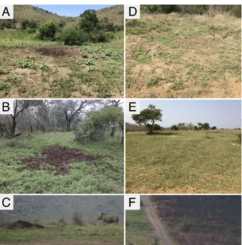
Figure 4. (A) Recently used midden in open woodland. (B) Recently used midden
in closed woodland. (C) Recently used midden on grazing lawn with sub-adult rhino. (D) Old, disused midden. (E) Grazing lawn in open habitat. (F) Burn scars from 2018 fires along the right side of the road. As seen here, roads frequently act as firebreaks.
3.1.2 Grazing lawn maps
Grazing lawn cover in 2004 was a significant predictor of grazing lawn cover in
2014 in 12 km2 grid cells, with 2014 lawn cover tending to be lower (R2 = 0.50,
estimate = 0.55, p < 0.001). Lawn cover in 2014 was a significant predictor of
lawn cover along road transects in 2018 in cold-spots for poaching (R2 = 0.25, p =
0.03, estimate = 0.6), but not in poaching hotspots (p = 0.7, R2 < 0).
3.2 Analyses
3.2.1 Middens as a proxy for rhino density
Rhino aerial census density in 2018 was a significant predictor of fresh midden
density along roads at the intermediate 12 km2 scale (p = 0.007), with an effect
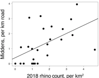
Extend-ing the model to all middens (as opposed to only fresh) improved model fit slight-ly (deviance explained = 27%), with effect size of 0.38 (p = 0.004) (Table 3; Fig-ure 5). Average long-term rhino density (as measFig-ured by the aerial census) was also predictive of all midden density (Table 3).
Figure 5. Midden density along park roads compared to 2018 rhino density,
mapped into grid cells of 12 km2. Quasi-poisson regression deviance explained =
0.27, p = 0.004.
The effect size for 2018 rhino density and midden density was larger at the larger
grid cell size (25 km2, effect size 0.80, 43% deviance explained). There was an
effect at smaller scales only for average rhino density over time (3 km2, 16%
devi-ance explained; Table 3). For modelling based on midden density (next section), I
used the 12 km2 grid cell size to have an adequate number of grid cells while
maintaining a strong relationship between middens and rhino.
Table 3. Relationship between rhino density and midden density, measured along
park roads in iMfolozi. Bold values are significant (p < 0.05). Grid
cell size
Generalised Linear Models
Quasi-Poisson offset by ln(Road Length / Cell Area) Spear
man’s Rho Model Effect Size p-value Deviance explained 12 km2 N = 25
Recent middens ~ 2018 census (rhinos/km2) 0.35 0.007 0.23 0.55
All middens ~ 2018 census 0.38 0.004 0.27 0.57
All middens ~ 2008-18 average (/annual total/km2) 2.9 0.04 0.14 0.41 3 km2
N = 42
Recent middens ~ 2018 census 0.15 0.1 0.04 0.13
All middens ~ 2018 census 0.14 0.09 0.04 0.17
All middens ~ 2008-18 average 1.6 0.003 0.16 0.41
25 km2 N = 15
Recent middens ~ 2018 census 0.68 0.002 0.34 0.67
All middens ~ 2018 census 0.80 0.007 0.43 0.80
3.2.2 Assessing white rhino habitat preference in HiP
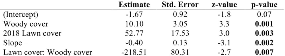
The best adequate model (BAM) in strictly-defined cold-spots (N=13) showed that recently used midden density was driven by slope, 2018 lawn cover, woody cover and the interaction between lawn and woody cover (Table 4). River cover and annual precipitation were highly correlated with other variables (VIF>3), so were independently tested in separate GLMs. The effects of fire frequency, annual pre-cipitation, river cover, and 2018 burn cover in explaining recently used midden density were insignificant (p > 0.05). Midden density increased at low slope and increased with increasing lawn cover, but only if woody cover was low. Maximum lawn cover is 19%, minimum woody cover is 20%, maximum woody cover is 60%, and minimum slope is 2.9˚.
The BAM in less strictly defined cold-spots (N=25) included slope, 2018 lawn cover, categorized woody cover, and the interaction between the two as significant explanatory variables for recently used midden density (Appendix Table 1). Road type was insignificant and excluded from the full model (Welch two-sample t-test p = 0.5). Fire frequency and annual precipitation were correlated with other ex-planatory variables (VIF>3) so were independently tested and insignificant (p > 0.05). Since equivalent variables were significant with comparable effect sizes to the more conservative definition of cold-spots employed in the first model, and since road type did not have a significant effect, the former model was accepted where cold spots were more stringently defined (Table 4).
Table 4. Summary table of the final fitted generalised linear BAM used to
quanti-fy habitat quality for rhino in 12 km2 grid cells in HiP cold-spots for rhino
remov-als (n = 13) with the response variable recently used midden count, offset by road length per grid cell. Significant values are in bold.
Estimate Std. Error z-value p-value
(Intercept) -1.67 0.92 -1.8 0.07
Woody cover 10.10 3.05 3.3 0.001
2018 Lawn cover 52.77 17.53 3.0 0.003
Slope -0.40 0.13 -3.1 0.002
Lawn cover: Woody cover -218.51 80.31 -2.7 0.007
Dispersion parameter = 1.3; for Poisson family taken to be 1. AIC: 49.85.
Null deviance: 29.362 on 12 degrees of freedom; Residual deviance: 10.433 on 8 degrees of freedom.
Deviance explained (Wood, 2006) = 0.645 Poisson model structure:
Recent midden count ~ Slope + Lawn cover + Woody cover + Lawn cover : Woody cover + offset ( ln (Road length) )
3.2.3 Assessing habitat quality of poaching hotspots in HiP
Across the entire park, the average habitat quality score was 2.84 ± 15.8, in pre-dicted midden density. The median score was 0.21. High quality grid cells were defined as those with scores above the third quartile, at 0.66; low quality grid cells had scores lower than the first quartile, 0.11.
The average quality score of poaching cold-spots was 2.3 ± 4.5 and of poaching hotspots was 0.38 ± 0.80. The variance in scores was higher in cold-spots than
hotspots (Bartlett test K2 = 42.164, p < 0.001), but means did not differ between
cold-spots and hotspots (Welch t-test p = 0.09; Table 5). Habitat quality scores by zone type across the park are plotted in Figure 6.
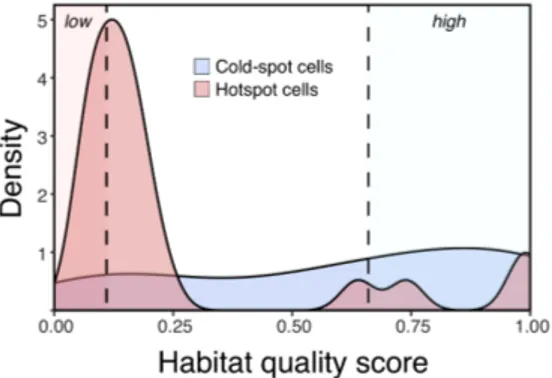
Figure 6. Approximate probability density curve of habitat quality scores by area
type in grid cells of size 12 km2. High quality grid cells were defined as those with
scores above 0.66 (the third quartile across all cells, right dashed line); low quality scores are lower than 0.11 (the first quartile across all cells, left dashed line). Scores above 1.0 were coerced to 1.0 for visualization.
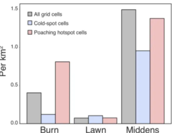
Two habitat variables differed significantly between cold-spots and poaching hotspot grid cells across the park: woody cover and fire frequency (Welch t-tests p < 0.05; Table 5; Figure 7). Poaching hotspot cells had less woody cover (p = 0.04) and burned more frequently (p = 0.001). Lawn cover and woody cover varied more in cold-spots (p = 0.04, p = 0.005; Table 4). Similar trends were found in the subset of grid cells that were measured on the roads transects (Appendix Table 2).
Table 5. Habitat measurements in cold-spots relative to hotspots across HiP at the
12 km2 grid cell size. Values are the mean and standard deviation across all cells
per poaching risk type. There were 15 cold-spots and 22 poaching hotspots across the park. Differences in means were tested using a Welch two-sample t-test. Dif-ferences in variance were tested using F variance tests and Bartlett tests; F ratio of variances compare cold-spots to hotspots. Significant values are in bold.
Cold-spots Poaching
hotspots
Welch t-test F test Bartlett test
t-value df p-value F p-value Bart-lett's K2 value p-2014 Lawn cover 0.12 ± 0.11 0.07 ± 0.07 1.9 27.1 0.07 2.6 0.04 4.2 0.04 Slope 5.4 ± 2.5˚ 5.7 ± 1.8˚ -0.4 30.0 0.7 2.0 0.1 2.3 0.1 Woody cover 0.28 ± 0.13 0.20 ± 0.057 2.2 22.2 0.04 5.3 0.005 12.1 0.001
Fire frequency 2.8 ± 2.6 yr 6.3 ± 3.7 yrs -3.6 37.3 0.001 0.5 0.1 2.1 0.1
Annual rainfall 587 ± 67 mm 614 ± 64 mm -1.3 35.8 0.2 1.1 0.8 0.03 0.9 River cover 1.0 ± 0.7 /km 0.8 ± 0.7 /km 0.9 36.2 0.4 1.0 0.9 0.004 0.9 Habitat score 2.29 ± 4.46 0.38 ± 0.80 1.8 17.9 0.09 31 0.001 42.2 0.001
Figure 7. Boxplots demonstrating habitat variable differences between cold-spot
(blue) and hotspot (red) grid cells. Stars indicate significant differences (Welch two sample t-test p < 0.05; Table 4).
3.2.4 Assessing rhino movement into poaching hotspots
3.2.4.1 Midden freshness
Along roads, 1.8 times as many middens per km were observed in poaching hotspots than cold-spots, and there were 1.4 times as many recently used middens per km, but the difference was not significant (t-test p = 0.06, p = 0.3, respective-ly). There were 3.5 times as many old middens per km in hotspots, which was significant (t-test p = 0.03). The ratio of old or disused middens to all middens was higher in hotspots than cold-spots for poaching (15.0% vs. 37.9%, p = 0.03) (Fig-ure 8).
Figure 8. Midden density in hotspot grid cells (red) as compared to cold-spot grid
cells (blue) along road transects. (A) Midden density overall did not differ (p = 0.06), nor did recently used middens (B) (p = 0.3). The density of old, disused middens (C) was higher in hotspot grid cells (p = 0.03). There are proportionally more old middens in hotspot grid cells (D & E) (p = 0.03).
3.2.4.2 White rhino population demography a) Population density
Prior to 2017, the proportion of the white rhino population per square kilometre was higher in hotspot than cold-spot grid cells (e.g., 2016 t = -2.3, p = 0.03; Table 6). In 2017, the peak year for poaching, the proportion of the white rhino popula-tion per square kilometre was significantly lower in poaching hotspot grid cells than in cold-spot grid cells (t = 3.0, p = 0.006). In 2018, it did not differ by risk type (t = 1.8, p = 0.08), and in no year did it differ by habitat quality (p > 0.1).
Table 6. White rhino population density (proportion of total iMfolozi Park
popula-tion) in hotspot grid cells (N = 15) relative to cold-spot grid cells (N = 13) based on census counts from 2008-2018. Rhino densities are proportional to the park total and to grid cell size. Differences in mean were tested using a Welch’s two-sample t-test. Significant values are in bold.
Year Rhino Density (%/km2) Welch t-test Cold-spots Poaching hotspots t-value p-value
2008 0.146 0.249 -2.0 0.06 2009 0.152 0.217 -2.1 0.04 2010 0.173 0.222 -1.1 0.3 2011 0.162 0.207 -1.2 0.2 2012 0.166 0.229 -1.6 0.1 2013 0.162 0.214 -1.2 0.2 2014 0.199 0.205 -0.1 0.9 2015 0.141 0.204 -1.9 0.07 2016 0.152 0.265 -2.3 0.03 2017 0.239 0.134 3.0 0.006 2018 0.226 0.141 1.8 0.08
While the total white rhino population has not changed significantly since 2008 (linear regression p = 0.8), the population in high quality cold-spots has grown (p
= 0.004, 0.09 rhinos/km2/year; Figure 9). If high quality cold-spots were
extrapo-lated across 555 km2 iMfolozi, this would mean an increase of 50 rhinos/year. In
hotspots for poaching, however, the population has declined (p = 0.02 in low
qual-ity, p = 0.04 in high qualqual-ity, -0.03 rhinos/km2/year in high and low quality,
extrap-olates to -17 rhinos/year across iMfolozi).
Figure 9. White rhino aerial count per square kilometre in cold-spot grid cells of
high (dark blue) and low quality (light blue) and hotspot grid cells of high (red)
and low quality (pink). Dots are the average rhino count per km2 in grid cells in
each category per year. Plotted lines are based on linear regression used to model
each habitat-quality/poaching risk combination (coloured lines) and for the park-wide average (dashed line). Grey bands indicate the 95% confidence interval. b) Colonisation rates
Per-capita colonisation was higher in high quality poaching cold-spots than in high quality hotspots (p = 0.04), but did not differ between high quality cold-spots and low quality hotspots (p = 0.9) or between high-quality cold-spots and low quality cold-spots (p = 0.1; Figure 10A; Table 7A).
Per-capita colonisation did not change through time in any area (p = 0.2). It ex-cluded four instances of infinite per-capita colonisation that occurred because zero rhino were counted in the previous year—one cold-spot grid cell in 2013, 2015, and 2016, and one poaching hotspot grid cell in 2018. Colonisation count (not scaled per capita) included these instances and did not differ significantly between any areas. Particularly noteworthy for my question, it did not differ between high quality hotspots and cold-spots (p = 0.99; Figure 10B).
c) Calf-adult ratios
Calf-adult ratios did not differ in high quality poaching hotspots relative to high quality spots (p > 0.9) or in low quality hotspots relative to high quality cold-spots (p > 0.9). In cold-cold-spots, calf-adult ratios were lower in low quality than high-quality areas (p = 0.02). Low high-quality cold-spots also had lower calf-adult ratios than high and low quality hotpots (p = 0.03 and p = 0.01, respectively; Figure 9C). Calf-adult ratios did not differ by quality within hotspots (p > 0.9). Further, calf-adult ratios did not change significantly through time in poaching hotspots of ei-ther quality (p = 0.2), or in any oei-ther grid cell type (p > 0.5).
d) Sub-adult proportion
Sub-adult proportion did not differ between high quality poaching cold-spots and high quality hotspots, low quality hotspots, or low quality cold-spots (p = 0.3, p = 0.5, p = 0.2, respectively; Figure 10D). Sub-adult proportion increased through time in high quality cold-spots (1.3%/year, p = 0.002), but did not change signifi-cantly through all years from 2008 to 2018 in poaching hotspots of either quality or low quality cold-spots (p > 0.05). From 2008 to 2017 (excluding 2018), howev-er, sub-adult proportion increased in all four quality-risk type combinations through time (1.4-2.0%, p < 0.03); the rate of increase did not differ by quality or risk type (p > 0.1).
Figure 10. Per-capita colonisation (A), colonisation count (B), calf-adult ratio (C),
and sub-adult proportion (D) averaged over 2008-2018 in cold-spot (blue) and hotspot (red) grid cells of high (dark) and low (light) quality. Dashed lines are park average rates, representing average year-year error in the aerial census. Stars at top represent significant differences from high quality cold-spots (p-values < 0.05) using generalised least squares modelling to fit each of A-D as a function of quali-ty and risk quali-type (Table 7).
Table 7. Simultaneous hypothesis testing of final generalised least squares models
for (A) white rhino per-capita colonisation, (B) calf-adult ratios, and (C) sub-adult proportion. CS = cold-spot grid cells, PHS = poaching hotspot grid cells, low = low quality grid cells, high = high quality grid cells. Estimates are the average over 2008-2018. Differences were tested using simultaneous tests for general line-ar hypotheses (‘multcomp’). Bolded values line-are significant (p < 0.05).
(A) Differences were tested between the hypothesized source area of high quality
cold-spots, and the three other quality-risk combinations.
A. Per-capita colonisation Estimate Std. Error z-value p-value
(Intercept) high.CS 2.01 0.35 5.76 <0.001
high.PHS - high.CS == 0 -0.81 0.35 -2.30 0.04
low.PHS - high.CS == 0 -0.18 0.48 -0.37 0.9
low.CS - high.CS == 0 -0.70 0.36 -1.95 0.1
Generalised least squares fit by REML:
Per-Cap Colonisation (non-infinite) ~ Quality.HS, weights = varIdent(form = ~1 | Quality.HS)) Variance function:
Different standard deviations per stratum Parameter estimates:
high*CS low*HS low*CS high*HS 1.00 0.80 0.14 0.11
AIC BIC logLik 41.65 46.17 -12.83 Standardized residuals:
Min Q1 Med Q3 Max -0.97 -0.71 -0.22 0.70 1.84 Residual standard error: 0.922
Degrees of freedom: 17 total; 13 residual
(B) Differences were tested between the hypothesized source area of high quality
cold-spots, and the three other quality-risk combinations, in comparison to (A), and between all other combinations to additionally test for compensatory repro-ductive rates.
B. Calf: adult ratio Estimate Std. Error z-value p-value
(Intercept) high.CS 0.090 0.007 12.023 <0.001 high.PHS - high.CS == 0 0.003 0.014 0.232 1.0 low.PHS - high.CS == 0 0.006 0.012 0.499 1.0 low.CS - high.CS == 0 -0.047 0.016 -2.955 0.02 low.CS - high.PHS == 0 -0.050 0.018 -2.770 0.03 low.CS - low.PHS == 0 -0.053 0.017 -3.180 0.01 high.PHS - low.PHS == 0 -0.003 0.014 -0.181 1.0
Generalised least squares fit by REML: Calf-adult ratio ~ Quality.HS
AIC BIC logLik -49.77 -46.95 29.89
Standardized residuals:
Min Q1 Med Q3 Max -1.35 -0.68 -0.12 0.68 1.46 Residual standard error: 0.01977203 Degrees of freedom: 17 total; 13 residual
(C) Differences were tested between the hypothesized source area of high quality
cold-spots, and the three other quality-risk combinations, the same hypotheses as (A).
C. Disperser proportion Estimate Std. Error z-value p-value
(Intercept) high.CS 0.21 0.01 14.93 <0.001
high.PHS - high.CS == 0 -0.04 0.03 -1.71 0.3
low.PHS - high.CS == 0 -0.03 0.02 -1.29 0.5
low.CS - high.CS == 0 -0.06 0.03 -1.99 0.2
Generalised least squares fit by REML: Disperser proportion ~ Quality.HS AIC BIC logLik
-33.50 -30.68 21.75
Standardized residuals:
Min Q1 Med Q3 Max -1.14 -0.70 -0.25 0.84 1.46
Residual standard error: 0.03696848 Degrees of freedom: 17 total; 13 residual
This study verified that poaching has the potential to create an ecological trap for the white rhinoceros in Hluhluwe-iMfolozi Park in South Africa.
1.) Fitness decreased through time in areas of the park that are at high risk for poaching (hotspots), and is lower than in low-risk areas (cold-spots) of equivalent resource quality.
2.) High quality habitat for white rhino in terms of resources differs through-out the park and is available in high-risk areas, and thus ecological theory suggests rhino will be drawn into high-risk, low fitness areas (Battin 2004).
3.) Rhino population density remains moderately high in high-risk areas de-spite poaching, though it can be argued that these rhino may have been there since before poaching began, or they were born into the high-risk ar-ea.
For an ecological trap to persist, rhino must actively move into high quality, high-risk areas at least as much (‘equal-preference’ trap) or more than (‘severe’ trap) other habitats (Battin 2004; Robertson & Hutto 2006). To exhibit avoidance, rhino must actively leave these areas. We were not able to confidently determine if ei-ther scenario was broadly applicable, but colonization rates suggest that rhino may avoid high-risk areas. Further discussion is provided below.
4.1 Fitness and resource quality mismatch in hotspots
White rhino density in iMfolozi, the section of HiP where the annual aerial census is conducted, decreased in hotspots for poaching but increased in cold-spots through time. Prior to 2017, the density of rhino was higher in hotspots than in cold-spots, but since 2017 it has been higher in cold-spots.
In this study, most high quality habitat occurred in grid cells in cold-spots for poaching in HiP. Nevertheless, I was able to identify high quality areas in
ing hotspots, and the aforementioned population decline in hotspots was independ-ent of quality level. In cold-spots for poaching there were low quality areas too, suggesting the existence of sink habitats. Thus further suggests that rhino leaving the low-risk high quality source could choose the high quality but high-risk hotspots instead of the low-risk sink habitat; if they do, an ecological trap is at play (Battin 2004).
My approach to defining habitat resource quality was to use only areas without rhino removals since rhino influence habitat structure, which has been especially well documented in HiP (Cromsigt & Olff 2008; Waldram, Bond & Stock 2008), though rhino presence plays a role even at lower densities (Cromsigt & te Beest 2014). In these cold-spot areas, grazing lawn availability, woody cover, and terrain slope factored into rhino habitat quality, which I measured using the density of rhino middens with fresh dung. These habitat variables have also been shown to be relevant for white rhino habitat preference in previous work (Pienaar 1994; Perrin & Brereton-Stiles 1999; Shrader, Owen‐Smith & Ogutu 2006; Waldram, Bond & Stock 2008; Cromsigt, Prins & Olff 2009).
It is possible that hotspots and cold-spots differ substantially in intrinsic environ-ment, to the extent that the cold-spot-fitted habitat quality model I produced may fail to accurately predict habitat quality in hotspots. Indeed, woody cover was lower, lawn availability was less variable, and fire frequency was much higher in hotspot areas. While I attempted to lessen this potential error by loosening the stringency of the cold-spot model, which gave a highly similar model, it is still conceivable that it underestimated hotspot habitat quality. A better route to avoid-ing this issue could have been to model rhino density before poachavoid-ing began across the whole park, as a function of habitat measurements from before then too, but unfortunately detailed rhino density data was only available starting in 2008. Plus, park management began translocating rhino out of HiP in the 1960s, so such an approach would be limited to areas of the park without management removals, or it would consider those negligible, which seems unreasonable (Player 1967; Rookmaaker & Antoine 2012).
I used a map of grazing lawn cover from 2014 (le Roux 2018), which was highly predicted by lawns in 2004. Since white rhino maintain grazing lawns (Waldram, Bond & Stock 2008), it is possible that rhino removals caused lawn cover to de-crease by 2018 relative to 2014, and this would likely be most evident in rhino removal areas. Indeed, in poaching hotspots, the 2014 lawn cover was not predic-tive of 2018 lawn cover, while it was in cold-spots, suggesting that lawn cover reduction may occur due to poaching. This suggests that modelled habitat quality in hotspots, which used the 2014 lawn cover map, might be too high. On the other hand, perhaps rhino are also drawn to habitats with the potential to support the grazing lawn ecotype. Even if lawns are not currently present, there are environ-mental factors like soil type, rainfall, termite activity, grass species availability, and local terrain that influence whether a lawn can develop (Gosling et al. 2012; Hempson et al. 2015), and these variables would not be rhino-dependent. Since rhino were poached before 2014, albeit at lower numbers, lawn cover in 2014 was
likely lower in hotspots than it had been prior to poaching. If rhino prefer areas with the potential to form grazing lawns, this could thus suggest the exact opposite trend—that, in poaching hotspots, actual habitat quality is higher than indicated by the model using 2014 lawn cover.
Furthermore, there is evidence suggesting that rhino are drawn to burnt grassland (T. Herkenrath, MSc thesis in prep). Like many other grazers, they may utilize the fresh regrowth of grass like Panicum and Themeda (Archibald et al. 2005). Fire frequency was not a significant predictor of habitat quality in the cold-spot model, but fire frequency in cold-spots was low overall. Since it was significantly higher in hotspots, I expect high fire frequency might mean rhino perceive resource quali-ty in hotspots as higher than predicted by the cold-spot model. Also, I measured long-term fire frequency, but rhino might be responding on shorter timescales to individual fire events – something that I could not detect using middens, which are more long-term, or aerial census counts, which are short-term but only once a sea-son. For these reasons, the habitat resource quality score in hotspots may be un-derestimated.
I used middens to define habitat quality because they are less transient than rhino density and could be linked spatially to habitat variables. In addition, measuring midden density had the benefit of being a non-invasive approach to studying rhino and their response to human threat. I showed that midden density was indeed cor-related with rhino density from the aerial census. However there are potential problems associated with that choice. Using middens as a proxy for rhino habitat quality assumes rhino spend most of their time in places similar to where their middens are. This is the case at least for territorial males and seems to be so also for other rhino (Owen-Smith 1975; Marneweck, Jürgens & Shrader 2018), but it is an important caveat of my method. It may create error, such as in the case of fire frequency: while rhino likely move temporarily to feed in burned areas, middens might not move correspondingly. Still, rhino are attracted to the habitat and at risk if it is in a poaching area. In future, rhino sightings along transects might be a use-ful corroboration of the midden density method, though this was not a feasible addition to this study due to unequal sampling time of day and low sighting count.
4.2 Rhino preference for high-quality cold-spots
Contrary to my hypothesis, per-capita colonisation was higher in cold-spots of high quality than in hotspots of high quality. This implies that rhino choose rela-tively safe areas of the park with high quality resources. As such, this suggests that an ecological trap may not describe the scenario in HiP. Further, since rhino can move into cold-spot habitats of high quality, these areas must not be at carrying capacity (Pulliam 1988), or, alternatively, it could indicate that most rhino do not compete over resources. Indeed, territorial males were the only group of rhino to exhibit competitive behaviour in HiP (Owen-Smith 1975). It is notable that the