OTHA - Omaha tools for hydrologic analysis - time-series/statistical analysis programs for water resources

Full text

(1)Hydrology Days 2004. OTHA – Omaha Tools for Hydrologic Analysis Time-Series/Statistical Analysis Programs for Water Resources William Doan, P.E.1 Hydraulic Engineer, U.S. Army Corps of Engineers, Omaha District,. Abstract. A suite of programs has been developed by the Omaha District to provide useful tools to aid in the rapid and accurate analysis of hydrologic daily flow time-series data and peak flow data for various water resources/environmental projects. These programs utilize tools not currently found in existing software and all the OTHA programs have: easy-to-use Visual Basic GUI interfaces, FORTRAN engines, connections to WEB data locations, data conversion utilities, and utilize standard data formats: HEC-DSS databases for daily flows and HEC-FFA input formats for instantaneous peak flows. Various water resources related routines within OTHA include: time-series cross-correlation analysis, trend analysis, volume-frequency/balanced-hydrograph generation, extension of records, synthetic daily flow and peak flow generation, mix-population analysis, total probability theorem analysis, risk/binomial distribution analysis, precipitation-frequency analysis using General Extreme Value 1 distribution, and tests and corrects for stationarity or linear trends of statistical parameters.. Model Development. The programs contained in OTHA are predominantly software that had been previously developed by the Omaha District Corps of Engineers in the course of analyzing various water resources projects. The primary purpose of OTHA was to compile all the existing programs into one easy-to-use package and to be able to use these programs in conjunction with traditional statistical analysis software such as HEC-FFA and HEC-STATS. Specific model goals include: 1. Provide direct access to data via the Internet. 2. Provide means to convert data into a standardized format (DSS for daily data and HEC-FFA input file format for instantaneous peak flow data). 3. Minimize amount of required data input. 4. Direct display of program output. 5. Provide for annual or seasonal analysis when using daily values. 6. Provide a common “look or feel” for all routines. 7. Provide useful set of tools for working engineers. Model Use. All routines within OTHA were written with FORTRAN and have Visual Basic graphical user interfaces. The routines within OTHA are called from a main menu or screen and are located within one of four main folders: 1. Hydraulic Engineer, U.S. Army Corps of Engineers, Omaha District, (402) 221-4583, bill.p.doan@usace.army.mil. ©Hydrology Days 2004.

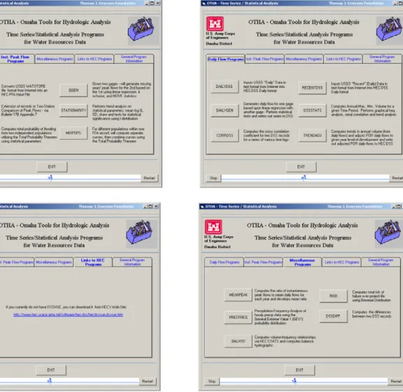
(2) Omaha Tools for Hydrologic Analysis. Figure 1. OTHA Main Menus The graphical user interface for each routine is shown below along with a brief description of each routine. For detailed descriptions of all routines, please refer to the OTHA Users Manual, which can be found at: http://www.nwo.usace.army.mil/hydro/hydrology/otha/index.html. 23.

(3) Doan, W.. Daily Flow Routines: DAILYDSS – Retrieves daily flow data from USGS Web-Site and converts the data into HEC-DSS daily time-series. The data from the Web Site needs to be saved as a “Tab-Separated Data File”. The name of the DSS file needs to be inputted, as well as the DSS pathname for the data to be placed in are required input.. 24.

(4) Omaha Tools for Hydrologic Analysis. DSSSTATS – Quickly and concisely summarizes a long-term period of record of daily flows for any period within a year into: annual minimum flows, annual maximum flows, annual mean flows, annual flow-volumes, annual lag-1 serial or autocorrelation coefficients, and computes graphical frequency-analysis, log-Pearson probability distribution, and trend analysis on annual maximum daily flow values with associated statistical significance tests. Writes out annual maximum flows to an FFA input file for further analysis.. 25.

(5) Doan, W.. ij. i i j j 1 N −k ij ck = ( ) ( )( ) = y y y y ck N ∑ r ii jj k t +k mean t mean (co co )1/2 i =1 ij. CORRDSS- Calculates the cross-correlation of two hydrologic daily timeseries using the cross-covariance between the two hydrologic time-series. (Salas, 1992) Essentially, determines the probability that two rivers will flood at the same time – useful for main/tributary confluences and interior drainage analysis. where: yi = one stream gage’s time-series of daily flows yj = another stream gage’s time-series of daily flows co= sum of the differences of daily flows from the mean of the daily flows, divided by the total number of observations t = time increment rk = lag-k cross-correlation coefficient c=cross-covariance between the two time-series k=times-series lag N=total number of values 26.

(6) Omaha Tools for Hydrologic Analysis. BALHYD – Serves as a graphical interface for HEC-STATS for flow volume-frequency analysis, then computes various return-interval symmetrical hypothetical “balanced” hydrographs and writes the ordinates out to HEC-DSS. Specific periods within the year can be computed, i.e. monthly or seasonal. The generated balanced 10, 25, 50, 100, and 500-year hydrographs are written to the specified DSS file.. 27.

(7) Doan, W.. Peak-Flow Routines: QWAT – Retrieves and converts USGS WATSTORE file format from the USGS’s Web Site into an HEC-FFA input file format (QR Cards).. 28.

(8) Omaha Tools for Hydrologic Analysis. EXTENSION - Extension of records or two-station comparison of peak flows. Utilizes the procedures described in Appendix 7 of Bulletin 17B for extending on gage’s record based on the concurrent period of a nearby gage. The program adjusts the log mean flow and standard deviation of the shortterm record based on the regression analysis with the long-term record. An inputted skew value can be used with the adjusted parameters to develop the final flow-frequency curve. (Hydrology Subcommittee, 1982). 29.

(9) Doan, W.. QGEN - Will generate individual year’s peak flows for a given station by comparison with nearby station. Will generate missing year flows by linear regression, linear regression with “noise”, and MOVE statistics. (Salas, 1991) The program puts the original data combined with the synthetic data into three FFA input files. y t = a + b( x t - µ t ) a=. (N 1 + N 2 ) µ y - N 1 µ y 1 N2. µ y = µY 1 +. α2 =. b2 =. σ y2 =. N2 σ ρ xy Y 1 ( µ X 2 − µ X 1 ) N1 + N 2 σ X1. N 2 ( N 1 − 4)( N 1 − 1) ( N 2 − 1)( N 1 − 3)( N 1 − 2). [( N 1 + N 2 - 1)σ y2 - ( N 1 - 1)σ Y21 - N 1 ( µY 1 - µ y ) 2 - N 2 ( a − µ y ) 2 ] ( N 2 - 1)σ X2 2. σ2 σ2 N1 N 2 1 ρ xy2 Y2 1 ( µ X 2 − µ X 1 ) 2 [( N 1 − 1)σ Y21 + ( N 2 − 1) ρ xy2 Y2 1 σ X2 2 + σ X1 N1 + N 2 − 1 σ X1 N1 + N 2. 30.

(10) Omaha Tools for Hydrologic Analysis. X is the set of annual peak flows for the long-term gage Y is the set of annual peak flows for the short-term gage µy and σy are the mean and standard deviation of the extended sequence yt is the variable with a missing variable to be generated µy1 is the mean of concurrent observations of Y ρxy is the cross-correlation between X and Y σy1 is standard deviation of concurrent observations of Y σx1 is standard deviation of concurrent observations of X σx2 is standard deviation of non-concurrent observations of X xt is the variable with the complete record µx1 is the mean of concurrent observation of X µx2 is the mean of non-concurrent observation of X N1 is the number of common observations between X and Y N2 is the number of values of Y to generate and:. MIXPOPS - For two physically-differentiated populations within one FFA record, the program will compute separate flow-frequency curves for each population then combines the two curves using the Total Probability Theorem. The curves are developed by converting the graphical plotting positions to a linear distance on the probability grid and solves for a best-fit line. (HEC, 1975) PCombined = PA + PB − PA PB where: PA = Probability of “A” occurring and PB = Probability of “B” occurring 31.

(11) Doan, W.. TOTPROB - Given the statistical parameters of mean log discharge, standard deviation, and skew for two different populations, the program will compute the log-Pearson Type III probability distribution for each, then combine the two curves for a smooth curve using the Total Probability Theorem. PCombined = PA + PB − PA PB. 32.

(12) Omaha Tools for Hydrologic Analysis. Miscellaneous Routines:. PRECFREQ - Precipitation-frequency analysis of hourly precipitation data using the General Extreme Value 1 probability distribution. The program sorts the hourly DSS records to determine the max “n-hour” for each year then computes graphical frequency analysis using the Weibull plotting positions as well as the GEV-1 analytical solution. Specific periods within the year can be computed, i.e. monthly or seasonal.. 33.

(13) Doan, W.. RISK - Computes the total risk of failure over a project life using the Binomial Probability Distribution (Chow, Maidment, Mays, 1988) based on the following equations: R = 1 − (1 −. 1 n ) T. n! P k (1 − P) n − k ( n − k )!k! where: R = Risk of occurance P = Probability in any year T = Recurrance interval K = Number of floods N = Number of years R=. 34.

(14) Omaha Tools for Hydrologic Analysis. MEANPEAK - Computes the ratio of mean daily flows to instantaneous peak flows given a FFA input file and mean daily flow DSS file. The programs takes the peak flow from the FFA input file for each year, then searches the mean daily flow DSS file to determine the corresponding mean daily flow for the day the instaneous peak flow occurred and computes the ratio. The program performs linear regression between the ratio of the peak flow to mean daily flow as a function of the mean daily flow or time.. 35.

(15) Doan, W.. STATIONARITY - Computes time-series of statistical properties of mean log discharge, standard deviation, skews, as well as the analytically-based 100year flow as a test for basin stationarity. Allows to see how the 100-year flow estimate changes with time and to readily see which statistical parameters influenced the changes. Performs trend-analysis on statistical parameters and tests the statistical significance of the trends using the Students t-test:. Test Statistic: bσ x N − 1 Tc = σε b = slope of regression curve σ x = standard deviation of parameter σ ε = standard deviation of residuals between actual values and regression values N = number of values Hypothesis test: b=0 is rejected if: Tc ⟩T1−α ( N − 2) where α is the 2. significance level.. 36.

(16) Omaha Tools for Hydrologic Analysis. TRENDADJ - Computes trends in annual flow volume (based on daily flows). If there is a trend, program will adjust the daily flows of the entire period-of-record to a given year level-of-development. The modified or adjusted period-of-record daily flows are written back out to HEC-DSS.. 37.

(17) Doan, W.. SAMSDSS – An interface that inputs stochastically generated monthly synthetic data generated by Stochastic Analysis, Modeling, and Simulation (SAMS) into HEC-DSS. Any combination of years of simulations and number of simulations will automatically be put into HEC-DSS where it may be directly utilized by other software, such as HEC-DSSVUE, HEC-5, or HEC-RESIM.. 38.

(18) Omaha Tools for Hydrologic Analysis. HEC Program Links:. A folder was created within OTHA to allow easy access to existing HEC programs. OTHA will make the links to the files if they are already loaded on the PC.. 39.

(19) Doan, W.. General Program Information:. A built-in User’s Manual, web-link, and mail link reside on the General Information Page.. Conclusion. All routines have example data sets, which are also the default values for the GUI interfaces. The routines within OTHA were developed by the Omaha District for various uses on water resources and environmental projects, but anyone may download and use the program. A link to the WebSite is found below: http://www.nwo.usace.army.mil/hydro/hydrology/otha/index.html. References Chow, Maidment, Mays (1988). Applied Hydrology. HEC (1975). Hydrologic Engineering Methods for Water Resources Development, Volume 3 Hydrologic Frequency Analysis. Hydrology Subcommittee (1982). Bulletin #17B – Guidelines For Determining Flood Flow Frequency.. 40.

(20) Omaha Tools for Hydrologic Analysis Salas, Jose D. (1991). Statistical Computer Techniques in Hydrology and Water Resources. Salas, Jose D. (1993). Handbook of Hydrology, Chapter 19 - Analysis and Modeling of Hydrologic Time Series. Salas, J.D., Saada, N., Chung, C.H., Lane, W.L. and Frevert, D.K., 2000, “Stochastic Analysis, Modeling and Simulation (SAMS) Version 2000 - User’s Manual”, Colorado State University, Water Resources Hydrologic and Environmental Sciences, Technical Report Number 10,Engineering and Research Center, Colorado State University, Fort Collins, Colorado.. 41.

(21)

No results found