View of Dynamics of Change and Change in Dynamics

(1)

2016, 2(1–2)

Published by the Scandinavian Society for Person-Oriented Research Freely available at

http://www.person-research.org

DOI: 10.17505_{/jpor.2016.05}

Dynamics of Change and Change in Dynamics

Steven M. Boker

1

_{, Angela D. Staples}

2

_{, Yueqin Hu}

3

1_{Department of Psychology, The University of Virginia} 2_{Eastern Michigan University}

3_{Texas State University} Contact

boker@virginia.edu

How to cite this article

Boker, S. M., Staples, A. D., & Yuegin, H. (2016). Dynamics of Change and Change in Dynamics. Journal of Person-Oriented Research, 2(1–2), 34–55. DOI: 10.17505/jpor.2016.05

Abstract: A framework is presented for building and testing models of dynamic regulation by categorizing sources of

differences between theories of dynamics. A distinction is made between the dynamics of change, i.e., how a system self–regulates on a short time scale, and change in dynamics, i.e., how those dynamics may themselves change over a longer time scale. In order to clarify the categories, models are first built to estimate individual differences in equilibrium value and equilibrium change. Next, models are presented in which there are individual differences in parameters of dynamics such as frequency of fluctuations, damping of fluctuations, and amplitude of fluctuations. Finally, models for within–person change in dynamics over time are proposed. Simulations demonstrating feasibility of these models are presented and OpenMx scripts for fitting these models have been made available in a downloadable archive along with scripts to simulate data so that a researcher may test a selected models’ feasibility within a chosen experimental design.

Keywords: dynamical systems analysis, multi-timescale analysis, self-regulation, person-oriented analysis

Dynamics of Change

Much recent work has concentrated on psychological pro-cesses that are hypothesized to exhibit regulatory dynam-ics. These processes typically change relatively quickly: Variables measuring these processes change over time scales of as short as milliseconds to as long as days. Pro-cesses hypothesized to exhibit regulatory dynamics include perception–action processes (Jeka, Oie, & Kiemel, 2000;

Wohlschläger, Gattis, & Bekkering, 2003), daily fluctu-ations in self-perceived mental health in recent widows (Bisconti, Bergeman, & Boker,2004,2006), self-disclosure and intimacy in married couples (Hamaker, Zhang, & van der Maas,2009;Laurenceau, Barrett, & Rovine,2005;

Laurenceau, Feldman Barrett, & Rovine,2005), symptoms of disordered eating in young women (Edler, Lipson, & Keel,2007), and positive and negative affect (Chow, Ram, Boker, Fujita, & Clore, 2005; Deboeck, Monpetit, Berge-man, & Boker, 2009; Zautra, Affleck, Tennen, Reich, &

Davis,2005). In each of these cases, some proportion of the observed short–term changes in observed scores are pat-terned in a time–dependent way that could reveal impor-tant clues about regulatory mechanisms. For the purposes of this article, the patterning of short–term change over time will be referred to as dynamics of change — the dynam-ical processes that are inferred from short term changes or fluctuations in time–intensive repeated observations. Most often, when authors write about the dynamics of a process, they mean the dynamics of change.

It is reasonable to think that there may be individual dif-ferences in the dynamics of change. That is to say, two indi-viduals may regulate in somewhat different ways. Individ-ual differences in the dynamics of change may take a variety of forms. The current article will categorize several types of individual differences in the dynamics of change and incor-porate them into a common modeling framework. In this way, parameters can be estimated and statistical tests can be performed for hypotheses concerning relationships

(2)

be-tween dynamics of change and other person–specific char-acteristics.

The dynamics of change can be studied using measure-ment bursts(Nesselroade, 1991); in other words, one or more sequences of repeated observations closely spaced in time with longer intervals between them. For instance, daily diary studies (Laurenceau, Barrett, & Rovine, 2005, e.g.,) and experience sampling methods (Bolger, Davis, & Rafaeli,2003;Cranford et al.,2006) can be considered ex-amples of burst measurement with only one burst. Methods such as time-delay embedding (Sauer, Yorke, & Casdagli,

1991;Oertzen & Boker,2010), latent differential equations (Boker, Neale, & Rausch, 2004), latent difference scores (McArdle,2001;Hamagami & McArdle,2007), Kalman fil-tering (Kalman,1960;Molenaar & Newell,2003;So, Ott, & Dayawansa,1994), dynamic factor analysis (Molenaar,

1985), and state–space (Chow, Hamaker, Fujita, & Boker,

2009) methods have been used to estimate parameters of the dynamics of change from burst measurement data.

If characteristics of the dynamics of change are constant over time, the dynamics are said to exhibit stationarity (see, e.g.,Hendry & Juselius,2000;Shao & Chen,1987, for dis-cussions of stationarity). This is a convenient assumption, as it means that for a selected individual any interval of time can be considered to be a representative sample of the dynamics of change for that individual. However, an as-sumption of stationarity frequently does not hold for psy-chological processes. Some processes, such as the dynam-ics of head movements during conversation (Ashenfelter, Boker, Waddell, & Vitanov, 2009; Boker, Xu, Rotondo, & King,2002), may be nonstationary during the same short time scales in which they exhibit their dynamics of change — that is to say these processes may exhibit nonstationary regulation. While such processes comprise an interesting category of psychological phenomena, they will be consid-ered as outside the scope of the current article. We will focus on a large category of phenomena where nonstation-arity is observed, but operates at a slower time scale than the dynamics of change for the process. This difference in temporal scale can be exploited to provide simultaneous es-timates of the short–term dynamics of change and longer term change in dynamics.

Change in Dynamics

Many psychological phenomena exhibit slow nonstationar-ity relative to their regulatory processes. Adaptation, learn-ing, or developmental processes are examples of nonsta-tionarity that could play out over a time scale of hours to decades. For instance, day–to–day or minute–to–minute emotional regulation may itself exhibit a developmen-tal trajectory, comprising within–individual differences in these regulatory mechanisms between childhood, midlife, and late life. Such a process may exhibit approximate lo-cal stationarity, that is to say over relatively short time scales, the characteristics of the dynamics of change may remain reasonably constant. However, over longer time scales, a process with approximate local stationarity can exhibit what will be referred to as change in dynamics —

relatively slow evolution of the parameters of the dynamics of change. We can take advantage of this difference in time scales to incorporate change in dynamics into existing mod-eling frameworks for individual differences in the dynam-ics of change so that hypotheses can be tested concerning the relationship of within–individual change in dynamics to other person–specific characteristics.

Two major categories of change in dynamics are: i) change in the equilibrium set for the process and ii) change in the attractor basin around the equilibrium set (Boker,

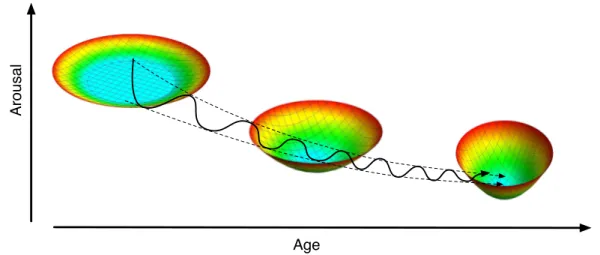
2013). The first category of change in dynamics is associ-ated with the equilibrium set, the set of equilibrium states, for a system. One simple and commonly used type of equi-librium set is a point equiequi-librium (or homeostatic equilib-rium) which is an equilibrium set with only one point in it. A point equilibrium means that there is one “best” or “optimal” or “goal” state for the system and that the system regulates relative to that state. There are many other types of equilibria (see, e.g., Hubbard & West, 1991, for a dis-cussion) including, for instance, a zone equilibrium where many values for a variable are equally good (Boker,2013). This so–called “comfort zone” is illustrated as the flat bot-tom of the leftmost of the three basins in Figure1. One way that long–term change in dynamics may occur is that there may be changes in the equilibrium set. For instance, there might be long term developmental change in the location of the centroid of the equilibrium, e.g, an individual’s average level of overall arousal might decrease from adolescence to mid–life. Another possibility is that the type of equilibrium set might change, e.g., from a point equilibrium to a zone equilibrium.

The second category of change in dynamics is defined by changes in the basin of attraction of the regulatory system and can be estimated as change in the parameters of the differential equation or difference equation that define the short–term dynamics of change. For instance, individuals might change in how they regulate — in adolescence a per-son might tolerate large swings in overall arousal while in mid–life that same person might exhibit much greater regu-latory control over their arousal levels as shown in Figure 1. In the arousal example for both categories of change in dynamics, short–term dynamics have stable regulatory characteristics, but over a longer timescale, these reg-ulatory dynamics may exhibit interesting and important change.

In order to estimate dynamics of change as well as change in dynamics, measurements must be sufficiently in-tensive in time to capture short term fluctuations as well as have sufficient longitudinal spread to be able to esti-mate developmental changes. Multiple burst designs are an efficient way to acquire these data. Sort bursts of time– intensive measurements (e.g., daily diary self–report or ecological momentary assessments) can be separated by longer intervals of time, e.g., months or years (e.g. Ong, Bergeman, & Boker,2009). In this way, change in dynam-ics may be estimated from longitudinal changes in within– individual parameters of the dynamics of change estimated from each burst. However, it may not be immediately ob-vious what these changes in dynamics might mean. The

(3)

Age

Aro

u

sa

l

Figure 1. A hypothetical arousal regulation system exhibiting two categories of change in dynamics. i) the equilibrium at young ages is a zone equilibrium set such that many similar levels of relatively high arousal are equally good and resulting in wide swings of arousal. In contrast, at older ages a point equilibrium emerges where there is a single best, and somewhat lower, level of arousal. ii) the attractor basin in the younger age is shown as having a flat bottom and shallow sides indicating a low degree of regulation while in older ages a steeper basin emerges indicating a greater degree of regulation around the equilibrium thus resulting in smaller arousal fluctuations.

next section builds an individual differences model for the dynamics of change a step at a time and discusses the mean-ings for individual differences in each of the parameters of the model. In this way, the stage is set for the last portion of the article which will discuss the meaning of within– individual change in these parameters and will present a model framework for estimating changes in dynamics si-multaneously with the dynamics of change.

Interindividual Differences in

Dynam-ics of Change

Let us consider three ways in which individuals may dif-fer in their dynamics of change: i) individual difdif-ferences in equilibria; ii) differences in amplitude of fluctuations; and iii) individual differences in the parameters of a selected model of the dynamics. One strategy to estimate the mag-nitude of individual differences in the dynamics of change is to allow particular coefficients of a chosen model to take on individual values for each person in a burst sample. The specifics of this strategy will be presented in a later section, but first let us examine the implications of individual dif-ferences in dynamics of change.

First, individuals may differ in their equilibria. For a se-lected variable, each individual may have a value around which they fluctuate. As an example, consider a study of cognitive abilities. On a day to day basis, a selected indi-vidual may perform better or worse on a cognitive task than her or his mean performance. Thus, for a cognitive perfor-mance variable, the mean perforperfor-mance over repeated ob-servations might be a reasonable estimate of a point equi-librium for each individual and the individual differences in within–person means could give an estimate of individ-ual differences in equilibria. Another example might be a

variable such as degree of intimacy a married individual feels with her or his spouse. Each individual husband or wife might have a preferred level of intimacy. Greater or lesser intimacy than the preferred level might be felt on any selected day and regulatory processes might keep the degree of intimacy somewhere near the equilibrium. But there may be individual differences within the class of hus-bands as well as within the class of wives. Also, within cou-ples, it may be that similarities or difference between the two spouses’ equilibrium values may be predictive of mar-ital satisfaction. Estimating and accounting for individual differences in equilibria is an important part of understand-ing regulatory systems.

Second, it may be that the amplitude of fluctuations around the equilibrium may differ across individuals. This might be due to individual differences in context or indi-vidual differences in regulatory dynamics. As an example of contextual differences, one person might be in a high– stress job whereas another person might be have a relaxed, low–stress occupation. The person in the high–stress job may have some days that are very difficult and troubling and other days that are fantastically rewarding. Each day for the person in the low–stress job may be quite like the day before: relaxing but not terribly rewarding either. In-dividual differences in contextual stressors for these two individuals might manifest as differences in amplitude of fluctuations in positive and negative affect. The affect of the person in the high–stress job is likely to show greater day–to–day fluctuations even if she is regulates her affect in a very similar way to the person in the low stress job. It is possible that the individual with the high stress job has self–selected her occupation in part due to her ability to effectively regulate stress. Whereas the individual in the relaxed occupation may be less able to regulate his affective fluctuations due to stress. Thus, the amplitude of observed fluctuations in affect may be due to both the contextual

(4)

ef-fects (the differences in stress levels of the job) as well as individual differences in regulatory dynamics. If these two individuals were to be presented with equivalent contexts, the same amount of stress may lead to small fluctuations in affect in the person who effectively regulates affect whereas it might lead to large fluctuations in affect for the person who does not regulate effectively. When modeling dynam-ics of change, it is important to be able to distinguish be-tween individual differences in context from individual dif-ferences in the model parameters controlling the dynamics. Third, there may be individual differences in regulatory dynamics. That is to say, the dynamics by which one person regulates may be somewhat different than it is for another person even after accounting for differences in equilibrium and differences in exogenous input. For instance, a large magnitude stressor might resonate for one person for a rel-atively long time, resulting in large fluctuations in affect that take weeks to die away. Whereas, for a second indi-vidual fluctuations associated with the same stressor might be damped within a matter of a day or two. Or, one person’s fluctuations might be rather slow relative to a second per-son. These individual differences in dynamics can be sub-stantively important and be related to other variables. For instance, in a study of recently–bereaved widows, Bisconti and colleagues (2006) found that how quickly fluctuations were damped was related to the degree of reported emo-tion focused coping provided by the widows’ social support network.

Intraindividual Change in

Dynamics

Let us now consider the same three sources of differences, but interpreted as ways in which the characteristics of an in-dividual’s regulatory dynamics might slowly change. Mod-els of change in dynamics must account for the fact that while individuals in a study are assumed to be indepen-dent of one another, a longitudinal model must be used to account for intraindividual change in dynamics.

The first way that intraindividual change in dynamics might occur is that the equilibrium value for the individual might shift over time. For instance, in a daily diary study, many recently bereaved widows exhibited a slow increase in a Mental Health Inventory (MHI) measure over a period of months (Bisconti et al.,2004). At the same time, these widows showed large daily fluctuations in MHI that could be modeled as a linear oscillator. The equilibrium point for the oscillations slowly changed over a period of months as the widows learned to deal with their loss.

A second possible way in which an individual’s regula-tory dynamics might change is that there could be a slowly evolving increase or decrease of amplitude of fluctuations about an equilibrium. For instance, an individual’s context may be changing across time and thus creating new exoge-nous input to the system. A job might become more stress-ful over time or retirement might change the pattern and frequency of stressors. In such cases, the regulatory dy-namics might stay constant while the observed amplitude

of fluctuations could increase or decrease. Changes in con-text are not necessarily examples of change in dynamics of regulatory systems. These changes might be entirely exter-nal to the regulatory system under study. However, when contexts are self–selected, one might consider contextual changes as part of a long–term adaptive strategy.

A third possibility is that one or more parameters for the selected dynamical systems model might change over time, implying that the regulatory dynamics are themselves changing. As an example, a younger individual might poorly regulate large fluctuations in mood, but later in life learn to become accomplished in such regulation.

Dynamical systems models are required to account for the regulatory process and longitudinal models are re-quired in order to account for long term within–person change. These models must be able to discern the differ-ence between changes in equilibrium, changes in external context, and changes in dynamics. Thus, a common frame-work is required that simultaneously models the dynamics of change and longitudinal change in dynamics. We will next provide a brief introduction of one common model for the dynamics of change, a second order linear differential equation. We will then extend this model to account for individual differences in equilibria, individual differences in the dynamics of change, and intraindividual change in dynamics.

Example Model: Second Order Linear

Differential Equation

Differential equations can be used for the specification of models for dynamical systems in psychology (e.g., Boker,

2012). These models specify a set of relations between the time derivatives of the variables involved in the regulatory system. The time derivative of a variable, written as ei-ther d x/d t or as ˙x, is the amount of change occurring in the variable at a specific moment in time. Thus, these dif-ferential equation models are quite literally models of the dynamics of change.

Linear second order differential equations have recently been used to model a variety of psychological processes. This model is intuitively appealing due to its correspon-dence to physical systems that have been used as metaphors for psychological systems. Continuously variable ther-mostats, pendulums, and springs may all be modeled to a first approximation with linear second order differential equations. As an example, psychological resilience is often described as the ability to “bounce back” from adversity. Hooke’s Law shows us that a simple model for elasticity with dissipation (akin to a bouncing ball that eventually comes to rest) is a linear second order differential equation (seeBoker, Montpetit, Hunter, & Bergeman,2010, for an extended discussion).

The linear second order differential equation for a vari-able x can be written as

¨

x(t) = ηx(t) + ζ˙x(t) (1)

(5)

equilib-rium. That is to say, the variable x is centered at its equi-librium point. When a variable’s equiequi-librium is fixed and known, we subtract that value from x to center the vari-able. When a variable’s equilibrium is unknown, a num-ber of strategies have been employed. We will discuss this question in greater detail in the next section.

Note that the parameters_{η and ζ have substantive} mean-ing. If_{η < 0, then one may say that the farther the system is} from equilibrium, the greater the acceleration that would turn it back towards equilibrium. Similarly ifζ < 0, one may say that the faster the system is changing, the greater the deceleration. As a way of intuitively grasping the im-pact of these parameters, it might be helpful to think about an automatic driver for a car. Ifη < 0 then the farther the car is from its garage (i.e., equilibrium), the more it tends to accelerate towards the garage. Ifζ < 0, then the faster the car is going, the more it tends to apply the brake.

This linear second order system has the interesting prop-erty that ifη < 0 and η + ζ2_{/4 < 0, then oscillations form.}

One may use the parameters of the equation to calculate the period of the oscillation (the time it takes for one full oscillation) asλ = p 2π

−(η+ζ2_/4). As will be seen in a later

section, this linear second order equation can be used to model a variety of dynamic behaviors.

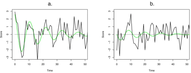
Figure 2 plots a time series for 50 measurements for two simulated individuals, a and b who have the same param-etersη = −0.3 and ζ = −0.1. However, a and b start at two different initial values. That is to say, at time t = 0, a’s score is 2.5 and b’s score is 0. The smooth curves are “true score” values that obey the regulatory dynamics of a second order linear differential equation. The noisy curves are just the smooth curve at each measurement occasion t > 0 plus a time–independent normally distributed ran-dom value with mean of zero and standard deviation of one. Note that if one were to take an average of a large sample of these curves, the “true scores” would cancel en-tirely since the initial starting point for each curve is a ran-dom value. Thus, a standard latent growth curve approach would completely miss the dynamics in these data and re-port that there was only time–independent residual error.

In order to estimate parameters of differential equations models from observed data, a number of techniques can be employed. Exact discrete (Singer,1993), approximate dis-crete (Oud & Jansen,2000;Oud,2007), and Kalman filter methods (Molenaar & Newell, 2003; Chow et al., 2009) can be used to estimate parameters of differential equation systems by first taking the integral and then estimating time lagged data. Another method, Latent Differential Equa-tions (LDE) (Boker et al.,2004;Boker,2007b,2007a) will be used here. Although the modeling framework presented in this article does not preclude using these other estima-tion methods, the specifics of model setup would be quite different than the examples presented here. At the core of the LDE method is time delay embedding, a time series technique that came to prominence in nonlinear dynami-cal systems analysis in physics (Sauer et al.,1991;Takens,

1985;Whitney,1936).

Time Delay Embedding

Time delay embedding is a preprocessing step that ensures that each row of one’s data set has encapsulated within it sufficient information to model the relevant dynamics of change. Then, an estimation method such as LDE or others can be used to model these dynamics. In essence, a short time–sequential snip of data is placed on each row. The starting point for each row is varied across all of the possible starting points for each individual. The number of columns in a snip is model dependent and data dependent, so this step takes some careful thought.

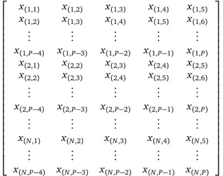
Suppose a time series X has been centered around each individual’s equilibrium values. If the original time series X is ordered by occasion j within individual i then the series of all observations x_(i,j)for N people, each of whom have been sampled P times, can be written as a vector of scores

X = {x_(1,1), . . . x_(1,P), x_(2,1), . . . x_(2,P), . . . ,

x_(N,1), . . . x_(N,P)}.

If we choose to create 5 columns in each snip, we can now construct a 5–dimensional time delay embedded ma-trix X(5)as                        x_(1,1) x_(1,2) x_(1,3) x_(1,4) x_(1,5) x_(1,2) x_(1,3) x_(1,4) x_(1,5) x_(1,6) .. . ... ... ... ... x_(1,P−4) x_(1,P−3) x_(1,P−2) x_(1,P−1) x_(1,P) x_(2,1) x_(2,2) x_(2,3) x_(2,4) x_(2,5) x_(2,2) x_(2,3) x_(2,4) x_(2,5) x_(2,6) .. . ... ... ... ... x_(2,P−4) x_(2,P−3) x_(2,P−2) x_(2,P−1) x_(2,P) .. . ... ... ... ... x_(N,1) x_(N,2) x_(N,3) x_(N,4) x_(N,5) .. . ... ... ... ... x_(N,P−4) x_(N,P−3) x_(N,P−2) x_(N,P−1) x_(N,P)                        .

Note that if one looks at the time delay embedded matrix column–wise, each column contains the time series lagged by an amount that is dependent on the column number. For instance, the second column contains almost the same data as the first column, except that it has been shifted up one row within each individual’s block of data.

The power of this method lies in the fact that each row of the matrix contains a sample of the time dependency information. One side–effect of this is that the ordering of the rows of a time delay embedded matrix does not af-fect an analysis since the time–dependent information has been captured within each row. This fact carries with it the great advantage that so–called phase resetting phenomena do not have large impacts on the parameter estimates of models fit from time delay embedded matrices (Deboeck & Boker,2010). A phase reset might occur when a substan-tial external event creates an abrupt change in the target variable value. The variable’s value is subsequently reg-ulated back towards equilibrium. Such phase resets are common in psychological data. For instance, a participant might be enrolled in a daily diary study of affect. On some

(6)

0 10 20 30 40 50 − 3 − 2 − 1 0 1 2 3

Eta=−0.3 Zeta=−0.1 DeltaEta=0 DeltaZeta=0

Time Score 0 10 20 30 40 50 − 3 − 2 − 1 0 1 2 3

Eta=−0.3 Zeta=−0.1 DeltaEta=0 DeltaZeta=0

Time

Score

a.

b.

Figure 2. Time series plots of 50 measurements of two simulated individuals, a and b. The smooth line is the underlying dynamic and the noisy line has time–independent error.

random day during the study, the participant has a minor car crash, causing a marked and abrupt disturbance to her affect. Over the next few days she regulates back to equi-librium. But then after another random interval, she wins a prize, creating a second disturbance in her affect for a few days. When we model affect, we are not interested in accounting for the interval between the car crash and the prize. This interval is not part of the affective regulatory system. Time delay embedding isolates these exogenous effects and balances their impact so that they induce lit-tle bias in estimating parameters of regulation (Oertzen & Boker,2010). However, time delay embedding carries with it a problem, in that the distribution of minus two times the log likelihood is not chi–square distributed. Until this problem is solved, standard error estimates for time delay embedding cannot be obtained by normal parametric meth-ods, but must be estimated by methods such as bootstrap-ping.

Second Order Latent Differential

Equation

As an example, we will restrict our discussion to variations on a linear second order Latent Differential Equation (LDE) for the dynamics of change of one variable (see Boker,

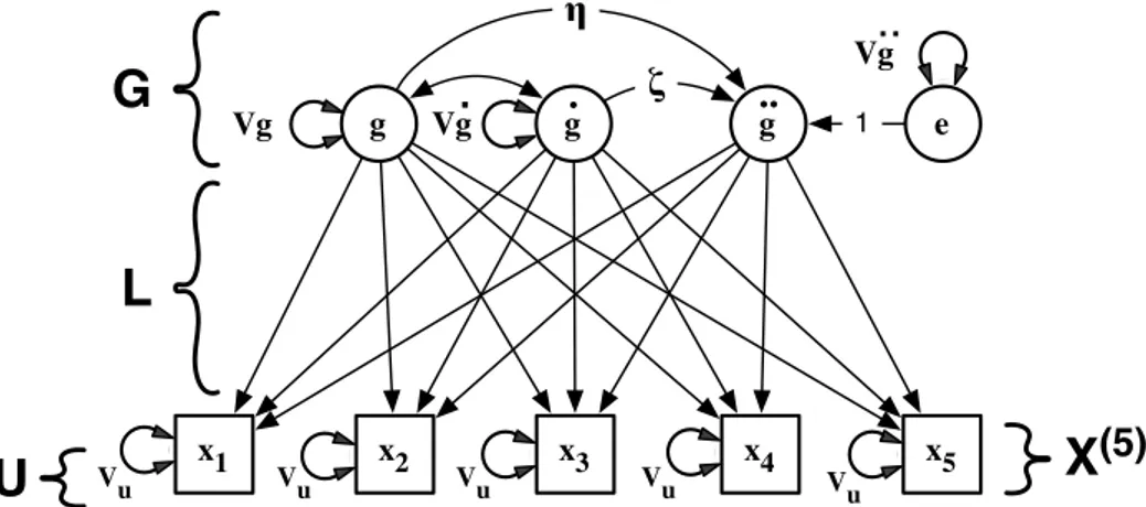
2007b, for a step by step introduction). By starting with a simple model, we can more easily focus later sections’ discussion on extensions that are necessary to account for interindividual differences in dynamics and intraindividual change in dynamics. Figure 3 presents a path diagram of the second order LDE of a variable x using a 5–dimensional time delay embedded matrix X(5). The latent second deriva-tive with respect to time, ¨g, for the jth row for person i in

X(5)is modeled as linear combination of the latent displace-ment, g, and its latent first derivative, ˙g,

¨

gi j = ηgi j+ ζ˙gi j+ ei j, (2)

where the residual term is assumed to be zero mean, inde-pendent, and identically distributed.

In matrix form, a second order LDE model for X(5)can be specified as

X(5) = GL + U, (3)

Where G is a matrix of unobserved latent derivative scores,

U is a matrix of unobserved unique scores and L is a fixed

matrix defined as L =      1 −2∆t (−2∆t)2_/2 1 −1∆t (−1∆t)2_/2 1 0 0 1 1_∆t _(1∆t)2_/2 1 2_∆t _(2∆t)2_/2      , (4)

where ∆t is the elapsed time between adjacent lagged columns in the time–delay embedded matrix X(5).

Fitting the model to data involves using the model– implied covariances between the columns of G to provide estimates of η and ζ, the residual variance for ¨g and for the covariance matrix for U, which is constrained to be diagonal with equal variances: a scalar matrix. We will use RAM structural equation modeling covariance algebra (McArdle & McDonald, 1984) and path diagram conven-tions (McArdle & Boker, 1990;Boker, McArdle, & Neale,

2002) to set up the model for the latent variables, speci-fying the covariance between columns of G as a product of asymmetric and symmetric paths contained in two matrices

A and S, A =   0 0 0 0 0 0 η ζ 0   (5) S =   V_g C_g_˙_g 0 C_g_˙_g V_˙_g 0 0 0 V_¨_g  , (6)

where Vg, V˙g, V¨g, and Cg˙gare the variances and covariances

of the latent variables g, ˙g, and the residual variance for ¨g. Now, the model implied covariance matrix, Cov(G), of the columns of the latent score matrix G can be calculated

(7)

x₁ x₂ x₃ x₄ x₅ g g

.

..

g V_u V_u V_u V_u V_u

ζ

η

e 1

L

Vg

..

Vg Vg

.

G

U

X

(5)

Figure 3. Path diagram of a second order linear latent differential equation model of a 5–dimensional time delay embedded matrix for a single variable. The latent second derivative, ¨g, is a linear combination of the latent displacement, g, and latent first derivative, ˙g.

as

Cov(G) = (I − A)−1S(I − A)−10. (7) When Cov(G) is scaled by the loading matrix L and added to the covariance matrix of U, the expected covariance matrix of X(5)can be written as

E (Cov(X(5))) = LCov(G)L0+ Cov(U) . (8) An example OpenMx (Boker et al.,2011) script to fit this second order linear LDE model using full information max-imum likelihood is presented in Appendix A.

Individual Differences in

Equilibrium

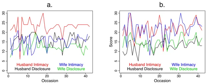
The model in the previous section assumes that each in-dividual’s data is centered around his or her own equilib-rium. This is can be reasonable if there is a known popu-lation equilibrium and there are no individual differences in this equilibrium value. However, for many psycholog-ical variables of interest, there are individual differences in equilibrium values and there is no a priori knowledge to guide us in centering individuals about their equilibria. Consider the data plotted in Figure 4 for two married cou-ples’ self–reported intimacy and disclosure scores over 45 days (Laurenceau, Barrett, & Rovine,2005). By inspection, each individual exhibits fluctuations about his or her own individual equilibrium for each variable.

One way to account for these individual differences in equilibrium value is to subtract a known or estimated equi-lbrium value from each individual’s time series. This pro-cess is sometimes called prewhitening or detrending in the time series literature. For instance, each individual’s mean over all occasions could be subtracted. But, it may be that the individual differences in equilibrium value are part of what one wishes to model. In this case it would be useful to be able to simultaneously estimate the equilibrium value and the parameters of the differential equation.

One way that individual differences in equilibrium values can be estimated simultaneously along with the parame-ters of an LDE is by adding a latent intercept term to the model as shown in Figure 5. This model is a hybrid of an intercept–only latent growth curve (LGC) model and a sec-ond order linear LDE and can be fit using full information maximum likelihood (FIML). The means for the data are modeled as a structured LGC while the variances and co-variances for the data are modeled as an LDE. This tech-nique essentially forces the LDE model for the dynamics to be fit to the residuals from the LGC means model where each individual can have their own estimated equilibrium value. Thus, we estimate the equilibrium value for each person that simultaneously maximizes the likelihood of the data given the chosen model for the dynamics. This simul-taneous estimation is an improvement over separately esti-mating individual means and centering each person’s data about the mean in a prewhitening step.

In the RAM path diagram notation (McArdle & McDon-ald, 1984; McArdle & Boker, 1990), variances are al-ways explicitly represented as double–headed arrows from a variable to itself. Note that the small circle near the bot-tom of Figure 5 has no variance. This small circle is simply a place holder to denote a matrix operation during estimation and not an actual latent variable. Also note that the arrow pointing from the triangle (constant) to the small circle is labeled as I|i, denoting that there are separately estimated intercept means (I) grouped (the vertical bar, |) by indi-vidual (i). Thus, the indiindi-vidual differences in equilibrium value are subsumed into the individually estimated mean parameters, one for each individual. There is one intercept value for each individual even though there are many rows in X(5) belonging to that individual. This is quite different than a standard growth curve model where the small cir-cle would be taken to be a latent intercept with a variance term that represented the individual differences. Here, it is the vector of parameters I|i that carry the individual differ-ences variance.

The model in Figure 5 can be written as

(8)

0 10 20 30 40 0 5 10 15 20 25 30 Occasion Score Husband Disclosure Husband Intimacy

Wife DisclosureWife Intimacy

0 10 20 30 40 0 5 10 15 20 25 30 Occasion Score Husband Disclosure Husband Intimacy

Wife DisclosureWife Intimacy

a.

b.

Figure 4. Intimacy and disclosure scores for two married couples (a and b) over 42 days of a daily diary study (data from Laurenceau, Barrett, & Rovine, 2005).

x

₁

x

₂

x

₃

x

₄

x

₅

g

.

..

g

u₁ u₂ u₃ u₄ u₅

1

I | i

ζ

e

1

L

K

U

M

_i

η

Vg

..

Vg

.

G

X

(5)

Figure 5. Hybrid linear second order LDE with individual differences in equilibrium intercept estimated by a latent intercept with mean grouped by individual.

(9)

where Mi is the ith row of an N× 1 matrix of means for

the N persons in the sample , K is a 1× D matrix with a fixed value of 1 in each cell, G is the latent derivative score matrix, L is the LDE loading matrix described in the previ-ous section, and Ui is a matrix of residuals for person i. In

the example shown in Figure 5, D= 5, since this example uses a time delay embedding data matrix with 5 columns. In general the optimal number of columns for time delay embedding will be dependent on the data and process to be estimated (see, e.g.,Hu, Boker, Neale, & Klump,2014, for techniques for estimating optimal D).

An example OpenMx script implementing this approach is shown in Appendix B and the individual equilibria from this simulation are plotted in Figure 7–c. This script takes advantage of novel features available in OpenMx in order to create a random parameters matrix (called “Rand” in the script). The matrix Rand has a row for each individual in the data set. This allows us to constrain the latent growth curve intercept to be equal within–individual but allows it to differ between individuals. In this way, estimates from the LDE part of the model can affect the latent growth curve part of the model which is grouped by individual.

A simulation was performed in which data were gener-ated to conform to the model in Figure 5 with small varia-tion in parameters between each of 100 replicavaria-tions. The data were generated according to an experimental design where 50 individuals were each measured on 50 occasions. Each individual’s equilibrium value was drawn from a nor-mal distribution with_{σ = 2.0. Each replication was then fit} using the model script in Appendix B and results are sum-marized in Table 1 and Figure 6. One data set did not con-verge and three data sets resulted in parameter estimates that were extreme outliers (> 100 standard deviations from the mean point estimate). These parameter values were clearly impossible given the structure of the data and could be easily excluded as being optimization failures. No at-tempt was made to adjust starting values and refit for the non-converging and extreme cases, instead these 4 cases were removed from the summary results in Table 1.

Individual Differences in

Equilibrium Change

One assumption of the model in the previous section is that there is no change in the equilibrium value during the burst of measurements. In many cases this assumption is rea-sonable, but in some cases it may not hold. For instance in Bisconti and colleagues’ study of recently bereaved wid-ows (Bisconti et al.,2004), there is good reason to believe that the equilibrium value was likely to be lower at the be-ginning of the 90 day study than it was at the end. Also, there was evidence of individual differences in this change in equilibrium value. This makes sense from a substantive standpoint since there are so many different possible cir-cumstances for a death. One death may be sudden and come as a great shock to surviving family members. An-other death may be after years of protracted illness and pain and survivors may find a sense of relief that a loved

one’s pain is finally over.

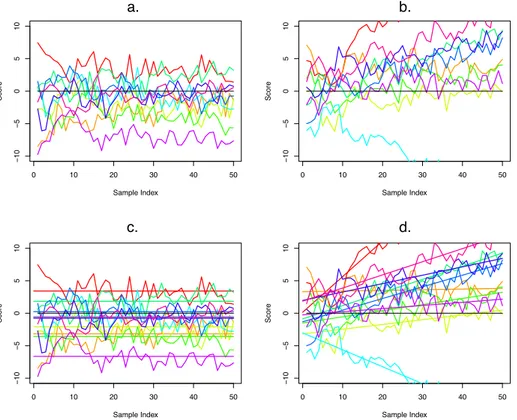
Figure 7 presents time series plots of two samples of sim-ulated data. In Figure 7–a there is no change in equilibrium value, consistent with the model from the previous section. But in Figure 7–b there are individual differences in not only the intercept, but also the slope of changing equilib-ria. Figures 7–c and 7–d show the results of fitting models allowing for individual differences in equilibrium and equi-librium change to the respective simulated data. The four plots in Figure 7 are produced as part of the scripts in Ap-pendix A and ApAp-pendix B.

Figure 8 presents a path diagram of a model that can simultaneously account for regulatory fluctuations and longer–term linear changes in equilibrium. The linear sec-ond order LDE portion of the model is unchanged from the previous model, but now we add a slope parameter, S|i, which is grouped by individual i. That is to say, the mean slope is constrained to be equal within–individual, but al-lowed to vary across individuals.

The model can be written in a similar form to the previ-ous model in Equation 9,

X(D)_i = MiK+ GL + Ui, (10)

but now Mi is the ith row of an N× 2 matrix of means

for the N persons in the sample and which contains the individual–specific means for the latent intercept and slope. The matrix K is a 2× D fixed matrix of values that allow the estimation of the latent intercept and slope. However, since the time delay embedded matrix X(D)_i has many rows for the same individual, while the matrix K is fixed for each row, its values must be calculated anew for each occasion j within each individual i’s block of data in X(D)_i .

If∆t is the interval of time between successive measure-ments in the D = 5 columns of X(5)_i , then one may pre– specify matrices two fixed value matrices, C and H such that C = ₁ ₁ ₁ ₁ ₁ −2∆t −∆t 0 ∆t 2∆t and H ₌ ₀ ₀ ₀ ₀ ₀ ∆t ∆t ∆t ∆t ∆t . (11)

For the jth occasion of measurement within individual i’s data, create a matrix J

J = 0 0 0 j . Now, one may calculate K as

K = JH + C. (12)

These row–specific calculations can be performed within OpenMx using its definition variable facility. Thus, if the occasion of measurement for each person is stored as a col-umn augmenting the time–delay embedded matrix, X(5)_{i j} , then the occasion of measurement, j, may be substituted into the matrix J for each row of a full information maxi-mum likelihood calculation. An example script is provided in Appendix C illustrating the use of individual–specific means and row–specific matrices to estimate this hybrid

(10)

Table 1. Simulation results for recovering individual differences in equilibrium value. Data were fit with the model shown in Figure 5 and scripted in Appendix B. The simulation includes 100 replications of an experiment with 50 individuals each measured on 50 equal-interval occasions. Standard deviations (sd) are the standard deviations of the simulated and estimated parameters.

Simulated (sd) Estimated (sd)

N 100 96

Did Not Converge 1

Extreme Outliers 3 Eta Mean -0.200 (0.014) -0.189 (0.016) Zeta Mean -0.100 (0.015) -0.110 (0.026) Intercept Mean -0.026 (0.289) 0.004 (0.311) Intercept Variance 4.081 (0.830) 4.641 (4.411) −0.24 −0.22 −0.20 −0.18 −0.16 − 0.24 − 0.22 − 0.20 − 0.18 − 0.16 Simulated Eta Estimated Eta ● ● ● ● ● ● ● ● ● ● ● ● ● ● ● ● ● ● ● ● ● ● ● ● ● ● ● ● ● ● ● ● ● ● ● ● ● ● ● ● ● ● ● ● ● ● ● ● ● ● ● ● ● ● ● ● ● ● ● ● ● ● ● ● ● ● ● ● ● ● ● ● ● ●● ● ● ● ● ● ● ● ● ● ● ● ● ● ● ● ● ● ● ● ● ● ● ● −1.5 −1.0 −0.5 0.0 0.5 1.0 1.5 − 1.5 − 1.0 − 0.5 0.0 0.5 1.0 1.5

Simulated Mean Intercept

Estimated Mean Intercept

● ● ● ● ● ● ● ● ● ● ● ● ● ● ● ● ● ● ● ● ● ● ● ●● ● ● ● ● ● ●● ● ● ● ● ● ● ●● ● ● ● ● ● ● ● ● ● ● ● ● ● ● ● ●●● ● ● ● ● ● ● ● ● ● ● ● ● ● ● ● ● ● ● ● ● ● ● ● ● ● ● ● ● ● ● ● ● ● ● ● ● ● ● ● ● −0.18 −0.16 −0.14 −0.12 −0.10 −0.08 −0.06 − 0.18 − 0.16 − 0.14 − 0.12 − 0.10 − 0.08 − 0.06 Simulated Zeta Estimated Zeta ● ● ● ● ● ● ● ● ● ● ● ● ● ● ● ● ● ● ● ● ● ● ● ● ● ● ● ● ● ● ● ● ● ● ● ● ● ● ● ● ● ● ● ● ● ● ●● ● ● ● ● ● ● ● ● ● ● ● ● ● ● ● ● ● ● ● ● ● ● ● ● ● ● ● ● ● ● ● ● ● ● ● ● ● ● ● ● ● ● ● ● ● ● ● ● ● ●

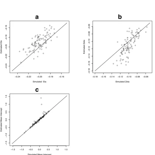
a

b

c

Figure 6. Scatterplots of simulated versus estimated parameters for a)η, b) ζ, and c) intercept for 96 replications of fitting the model

(11)

0 10 20 30 40 50 − 10 − 5 0 5 10 Sample Index Score 0 10 20 30 40 50 − 10 − 5 0 5 10 Sample Index Score 0 10 20 30 40 50 − 10 − 5 0 5 10 Sample Index Score 0 10 20 30 40 50 − 10 − 5 0 5 10 Sample Index Score a. b. c. d.

Figure 7. Time series plots of data with (a) individual differences in mean equilibrium and (b) individual differences in both intercept and slope of the equilibrium. Individual differences in equilibria are shown as lines resulting from (c) fitting the model from Equation 9 and (d) fitting the model from Equation 10. LDE parameters are simultaneously estimated from the residuals of these estimated equilibria.

x1 x2 x3 x4 x5 g g

.

..

g 1 I | i S | i

ζ

η

e 1

L

K

_t

M

_i

u₁ u₂ u₃ u₄ u₅

U

Vg

..

Vg Vg

.

G

X

(5)

Figure 8. Hybrid linear second order LDE with individual differences in equilibrium intercept and slope estimated by latent intercept and slope terms with means grouped by individual.

(12)

LDE and LGC model and individual equilibria for the first 10 individuals from this simulation are plotted in Figure 7– d.

A second simulation was performed in which data were generated to conform to the model in Figure 8 with small variation in parameters between each of 100 replications. The data were once again generated according to an exper-imental design where 50 individuals were each measured on 50 occasions. Each individual’s equilibrium intercept and slope was drawn from a normal distribution with in-terceptσ = 2.0 and slope σ = 0.3. Each replication was then fit using the model script in Appendix C and results are summarized in Table 2 and Figure 9. Five data sets did not converge and two data sets resulted in parameter estimates that were extreme outliers. Again, the non-converging and extreme outlier cases were removed from the summary re-sults.

Individual Differences in

Dynamics

The models presented in the three previous sections do not take into account the possibility that individuals may dif-fer from one another in the way they self–regulate, that is to say there may be individual differences in the shapes of the systems’ basins of attraction. In many regulatory sys-tems it may be expected that there will be measurable in-dividual differences in the parameters of models of regula-tion and that these individual differences would be substan-tively important. For instance, variables such as resiliency in older adults (Montpetit, Bergeman, Deboeck, Tiberio, & Boker, 2010), disclosure and intimacy in married cou-ples (Laurenceau, Rivera, Schaffer, & Pietromonaco,2004), and hormone cycles and disordered eating in young women (Edler et al., 2007) all have shown evidence of substan-tively important individual differences in the parameters of dynamical models.

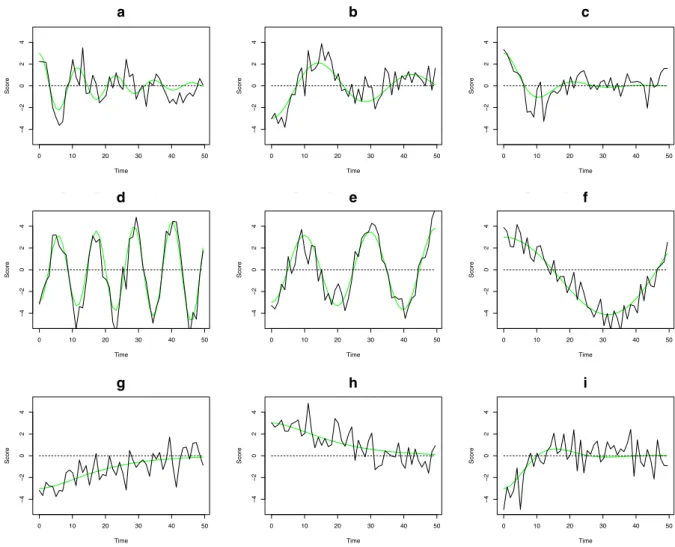
Figure 10 presents nine examples of how different tra-jectories can result from parameter differences in a second order linear differential equation. In each of these time series plots, the same equation is used and only the param-eters and starting values are changed. These plots illus-trate how seemingly different behavioral trajectories may result from a single underlying differential equation pro-cess. Figures 10–a, 10–b, and 10–c are oscillating systems with damping. That is to say oscillations tend to die out over time if they are not perturbed by external events. Fig-ures 10–d, 10–e, and 10–f are oscillating systems with am-plification; systems that tend to amplify perturbations from exogenous sources. Finally, Figures 10–g, 10–h are over-damped, and 10–i is nearly overdamped. These systems show trajectories that seem very similar to a first order lin-ear system with exponential decay.

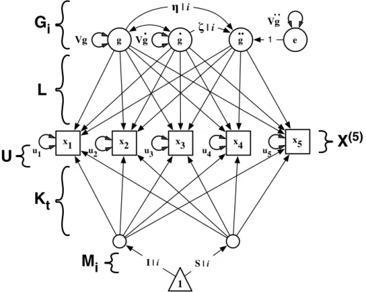
We can make an adjustment to the model from the previ-ous section in order to estimate individuals’ parameters of the LDE as shown in the path diagram in Figure 11. This adjustment requires individual level subscripts on the LDE

model equations which can be written, ¨

gi j = ηigi j+ ζig˙i j+ ei j (13)

X(5)_{i j} = MiK+ GiL+ U. (14)

This model can be implemented in OpenMx using the same mechanism that we used to group the intercepts and slopes by individual. We add two new columns to the random pa-rameters matrix and use the individual ID as an index into the random parameters matrix in order to constrain_ηiand

ζi within–individual while allowing individual differences

in these parameters. An OpenMx script implementation is shown in Appendix D.

A third simulation was performed in which data were generated to conform to the model in Figure 11 where each individual’s parameters of the second order differen-tial equation were drawn from a normal distribution with means and variances shown in Table 3. The data were again generated according to an experimental design where 50 individuals were each measured on 50 occasions. Each in-dividual’s equilibrium intercept and slope was drawn from a normal distribution with intercept σ = 2.0 and slope σ = 0.3. Each replication was then fit using the model script in Appendix D and results are summarized in Table 3 and Figure 12. All data sets converged and one data set re-sulted in parameter estimates that were extreme outliers. Again, the non–converging and extreme outlier cases were removed from the summary results.

Individual Differences in

Variability

Another important and often studied source of individual differences is variability. Variability is sometimes opera-tionalized as the within–person variance (or standard de-viation) of repeated observations of a variable. However, this definition misses an important distinction: the differ-ence between the overall amplitude of the displacement from equilibrium and the amplitude of the first derivatives (Deboeck et al.,2009). This distinction is illustrated in Fig-ure 13.

Both of these types of variability may be estimated by allowing individual differences in the variances of the dis-placement and first derivatives. Thus, the path model from the previous section can be relaxed further as shown in Figure 14 where V g|i and V ˙g|i are the variances of the displacement from equilibrium and first derivatives respec-tively grouped by individual i. This model can be imple-mented in OpenMx in the same manner as was used in mod-eling individual differences in the parameters of the differ-ential equation. While we do not show this in an Appendix, a script implementing this is included in the downloadable archive file.

Second Level Predictors

When there are individual differences in parameters of a dynamical systems model, it may be of interest to predict

(13)

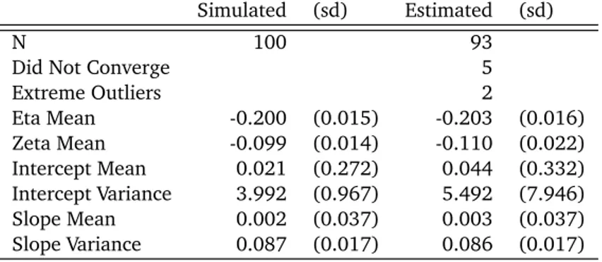
Table 2. Simulation results for recovering individual differences in equilibrium value and equilibrium change. Data were fit with the model shown in Figure 8 and scripted in Appendix C. The simulation includes 100 replications of an experiment with 50 individuals each measured on 50 equal-interval occasions. Standard deviations (sd) are the standard deviations of the simulated and estimated parameters.

N 100 93

Did Not Converge 5

Extreme Outliers 2 Eta Mean -0.200 (0.015) -0.203 (0.016) Zeta Mean -0.099 (0.014) -0.110 (0.022) Intercept Mean 0.021 (0.272) 0.044 (0.332) Intercept Variance 3.992 (0.967) 5.492 (7.946) Slope Mean 0.002 (0.037) 0.003 (0.037) Slope Variance 0.087 (0.017) 0.086 (0.017) −0.24 −0.22 −0.20 −0.18 −0.16 − 0.24 − 0.22 − 0.20 − 0.18 − 0.16 Simulated Eta Estimated Eta ● ● ● ● ● ● ● ● ● ● ● ● ● ● ● ● ● ● ● ● ● ● ● ● ● ● ● ● ●● ● ● ● ● ● ● ● ● ● ● ● ● ● ● ● ● ● ● ● ● ● ● ● ● ● ● ● ● ● ● ● ● ● ● ● ● ● ● ● ● ● ● ● ● ● ● ● ● ● ● ● ● ● ● ● ● ● ● ● ● ● ● ● −1.5 −1.0 −0.5 0.0 0.5 1.0 1.5 − 1.5 − 1.0 − 0.5 0.0 0.5 1.0 1.5

● ● ● ● ● ● ● ● ● ● ● ● ● ● ● ● ● ● ● ● ● ●●● ● ● ● ● ● ● ●● ● ● ● ● ● ● ● ● ● ● ● ● ● ● ● ● ● ● ● ● ● ● ● ● ● ● ● ● ● ● ● ● ● ● ● ● ● ● ● ● ● ● ● ● ● ● ● ●● ● ● ● ● ● ● ● ● ● ● ● ● −0.15 −0.10 −0.05 0.00 0.05 0.10 0.15 − 0.15 − 0.10 − 0.05 0.00 0.05 0.10 0.15

Simulated Mean Slope

Estimated Mean Slope

● ● ● ●● ● ● ● ● ● ● ● ● ● ● ● ● ● ●● ● ●● ● ● ● ● ● ● ● ● ● ● ● ● ● ● ● ● ● ● ●● ● ● ● ● ●● ● ● ● ● ● ● ● ● ● ● ● ● ● ● ● ● ● ● ●● ● ● ● ● ● ● ●● ● ● ● ● ● ●●● ● ● ●● ● ● ● ● −0.14 −0.12 −0.10 −0.08 −0.06 − 0.14 − 0.12 − 0.10 − 0.08 − 0.06 Simulated Zeta Estimated Zeta ● ● ● ● ● ● ● ● ● ● ● ● ● ● ● ● ● ● ● ● ● ● ● ● ● ● ● ● ● ● ● ● ● ● ● ● ● ● ● ● ● ● ● ● ● ● ● ● ● ● ● ● ● ● ● ● ● ● ● ● ● ● ● ● ● ● ● ● ● ● ● ● ● ● ● ● ● ● ● ● ● ● ● ● ● ● ● ● ● ● ● ● ●

a

b

c

d

Figure 9. Scatterplots of simulated versus estimated parameters for a)η, b) ζ, c) intercept, and d) slope for 93 replications of fitting the model shown in Figure 8 using the script in Appendix C.

(14)

0 10 20 30 40 50 − 4 − 2 0 2 4

Eta=−0.3 Zeta=0.02 Int=0 Amp=−3