Performance assessment of Apache Spark applications

(1)

Author:

Salam Al Jorani

Supervisor:

Diego Perez

Semester:

VT/HT 2018

Subject:

Computer Science

Bachelor Degree Project

Performance assessment of Apache

Spark applications

(2)

Abstract

This thesis addresses the challenges of large software and data-intensive systems. We will discuss a Big Data software that consists of quite a bit of Linux configu-ration, some Scala coding and a set of frameworks that work together to achieve the smooth performance of the system. Moreover, the thesis focuses on the Apache Spark framework and the challenging of measuring the lazy evaluation of the trans-formation operations of Spark. Investigating the challenges are essential for the per-formance engineers to increase their ability to study how the system behaves and take decisions in early design iteration. Thus, we made some experiments and mea-surements to achieve this goal. In addition to that, and after analyzing the result we could create a formula that will be useful for the engineers to predict the performance of the system in production.

(3)

1 Introduction

This thesis studies the performance of an industrial application that executes using Apache Spark [1], a Big Data framework for Data Intensive applications. This application exe-cutes in the context of e-government and tax fraud detection. In order to study the perfor-mance of the application, we instrument its source code and measure its execution time. Later, we analyze the measurement results, propose and validate a method which will be used to estimate the performance of the application in other situations that cannot be measured at present (i.e., to predict its performance at production). This method will be parametric with respect to the size of the input data to compute by the application.

Due to the novelty of Apache Spark framework and its performance particularities, this performance characterization process has not been straightforward. On the contrary, I have needed to understand the internal execution and some particularities of Apache Spark and to face several measurement challenges using this framework. Therefore, the reader will also get an overview of one of the fastest and scalable frameworks for Data Intensive Applications.

1.1 Background

Governments are losing a huge amount of money every year because of tax frauds. The European Union has estimated the financial loss due to tax evasion to be of the order of 1 trillion euros [2]. There is, therefore, a need to develop systems capable of detecting tax fraud. BigBlu is one of these systems and is under development by Netfective Tech-nology. Big Blu uses Apache Spark framework for its data analysis, and there is a need for the prediction of BigBlu performance in production when it receives large datasets to analyze. Therefore, the background of this thesis covers the knowledge of BigBlu itself, the characteristics of Apache Spark framework, and concepts of performance evaluation and performance measurement of software systems.

1.1.1 Apache Spark

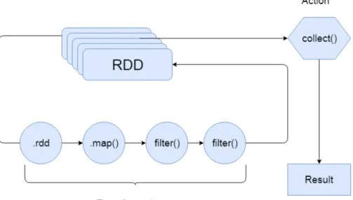
Apache Spark is one of the most used frameworks for Big Data analysis. Spark offers a set of operations which can be separated into two groups, called transformations and actions [3]. Operations of type transformation transform data into another data. For example, filter()and map() are the most basic and widely used transformations. In turn, an action operation is performed when we want to work with the dataset that has been created by a transformation. Some examples of operations of type action of the Spark are count(), reduce(), collect(), take(),... .[4].

Given a workflow of operations, Spark creates a DAG (Direct Acyclic Graph) with them [5], and executes the graph in order. One of the particularities of the execution of the workflow of operations is that transformation operations are “lazy”. Lazy means that these operations do not execute as soon as the execution of the workflow reaches them, but they wait until an action operation is reached in the workflow. At that moment, all transformations and the action execute together. In other words, the action operation is the trigger for the execution of the workflow of precedent operations.

1.1.2 BigBlu

BigBlu is a Big Data industrial application based on Apache Spark framework which is under development for an e-government Tax Fraud Detection system [2].

(5)

This thesis works on the functionality called “Launch Fraud Detection” of BigBlu. As Figure 1.1 illustrates, this functionality is composed of operations that 1) read the dataset from a Cassandra database, 2) perform a map transformation on the data that has been read in order to create a set of tuples with which it is easier to work, 3) apply filtering with conditions to these tuples to unveil anomalies in the tax declaration of taxpayers, 4) collect the resulting dataset from the filtering, and 5) write the results to the output Cassandra database.

1.1.3 Performance measurements and performance engineering

The Performance Engineer of BigBlu project has the current version under development and needs to estimate how the application behaves in production. This thesis contributes to this task.

Traditionally, for characterizing the performance of an application, there are carried out performance measurements of each activity in its workflow. This is, the application is measured with different inputs, and getting the starting and finishing timestamps of each activity. With these timestamps, it is possible to split the total execution time of the application into the time demanded by each activity.

However, this process cannot be followed for measuring Apache Spark performance. The lazy execution of the transformation operations of Apache Spark makes the perfor-mance measurement challenging.

This lazy behaviour of transformations and their combined execution with subsequent action causes major difficulties to measure the performance of each operation in the work-flow. It causes that we cannot follow a straightforward instrumentation of the code and gathering of timestamps because transformation operations do not execute in their corre-sponding position in the source code. Therefore, in order to obtain performance measure-ments of each of the operations in a Spark workflow, we need to instrument the code of Big Blu in a more complex manner, adding auxiliary actions and performing experiments in series of partial and incremental workflows.

(6)

1.2 Related work

This thesis is related to a previous research work with BigBlu, developed by Netfective Technology, which focussed on performance within its DevOps process rather than on the performance of the Spark operations [6]. That work focussed on how to achieve the performance requirements during development iterations.

BigBlu has been studied and partially developed within the DICE H2020 European project [7]. One of the parts of DICE project was the performance modelling of different frameworks for developing Data Intensive applications, such as Apache Hadoop, Storm and Spark. These performance models were used, for instance, for calculating the neces-sary amount of computing resources for a given application or for what-if analysis if the execution conditions or operational profile of the application changed. In this thesis, we study how to make performance measurements on running systems so the parameters of their performance models regarding the execution times of activities can be populated. 1.3 Problem formulation

Apache Spark applications execute a workflow of Spark operations (also called DAG). For instance, having a workflow of operations to detect the average income for France citizens with a specific age range, then this workflow will consist of multiple ordered Spark operations like filter, map, reduce etc. Each of these operations consume time and resources to do their jobs. The accurate measurement of the resource demand of each operation is essential for evaluating the performance of the Spark workflow and predicting its performance in other environments (in our case, in the future production environment). Thus, we need to know how well the workflow of Spark operations works and how many resources it consumes.

Unfortunately, the performance characterization of Spark operations is right now a very challenging task for the Performance Engineer, for instance, due to its so-called lazy operations. Even being challenging, these performance engineering activities are necessary to estimate how the system will behave in production. For instance, when it needs to process the massive amount of data in each execution. Moreover, in future when some conditions such as the frequency of executions requested from users varies or several databases from different geographical regions considered for the tax fraud analysis.

Therefore, there is an important problem to solve on the performance characterization of Spark applications in general. In this project, we contribute to measure the execu-tion times of the Spark operaexecu-tions in a concrete Case Study, Big Blu, and to estimate its performance in different environments.

1.4 Motivation

This problem is important from the industrial perspective. Understanding the performance of the Spark operations, allow releasing to production applications of good quality faster. Big Data applications are dealing with databases, which are:

• too big volume, for example, millions of tax operations every day with history data. • too diverse, for this specific project, the data can be from different sources, for

instants (incomes, VAT, banks...)

(7)

Thus, any attempt to discuss the performance prediction problem will lead to increase the throughput of the development of the application. My case study application, Big Blu, targets a big tax data that manage a countrywide area. Releasing Big Blu with poor performance - or that it collapses due to scarcity of resources - will be unusable by tax inspectors as it would incur in an unaffordable waste of their time. Besides, I wanted to gain some experience regarding Performance Engineering concepts.

1.5 Objectives

Due to the lack of previous experience in Apache Spark environments and Scala language, I have targeted a large set of subobjectives that, put together, allow to the achievement of the performance study.

O1 Study the Apache Spark framework in general and its lazy transfor-mation in particular.

O2 Set up the infrastructure of an industrial case study for Tax Fraud Detection that uses Spark Platform and Cassandra Database.

O3 Study the code of the case study and identify the relevant parameters for the performance of the application.

O4 Characterize the performance of each operation in the application workflow using different combinations of values of the relevant pa-rameters identified in (3) (the characterization of some Spark opera-tions is a challenging task due to their lazy execution).

O5 Study the overhead of Spark platform itself by executing an "idle" application (an application whose operations are empty and therefore they do not demand CPU) under different configurations of the Spark Framework (e.g., different number of worker nodes).

O6 Using the outputs obtained in (3) and (4), create a model that rep-resents the information obtained. This task enables further model-based performance evaluation of the application, without needing to re-execute it (which is a very time consuming task).

O7 Try to generalize what I have learnt on performance characteriza-tion and Performance Engineering of the Tax Fraud case study to any Spark application.

After achieving these objectives, we will be able to characterize the performance prop-erties of the constituent operations of an Apache Spark workflow. Then, I can make eval-uations of the system in different siteval-uations using the measured information. Moreover, I will reflect on generalizing this solution and make it applicable for different Spark appli-cations.

1.6 Scope/Limitation

To limit the scope of the project, this study focuses on the execution of Big Blu in typical Virtual Machines running OS Ubuntu. The cluster of Spark resources consists of homo-geneous virtual machines. The study focuses also on a single version of Spark and uses its basic configuration.

Fine tuning of the configuration of parameters of Big Data technologies is a challeng-ing task that requires much expertise which probably will not be available at the company;

(8)

there have been more companies which wished to develop Big Data applications than Big Data Developers and Operations experts [8] . Then leaving aside the fine-tuning of the many parameters of Apache Spark that might affect its performance. The reason is that the focus of the thesis is not to improve the performance of a Spark application, but to be able to predict such performance at design and implementation time. Therefore, for the aim of the thesis, a basic configuration of Spark suffices. Moreover, the focus of the research part of the project consists of characterizing and modelling the performance of Spark workflows only at the software operation level. It means that, for instance, the per-formance of the used Hard Drive technology and configuration, as well as the network bandwidth and latency, are out of the scope of this project. On the one hand, two impor-tant research challenges in this project are a) to measure the effect and b) to model the performance of the Lazy operations in Spark.

1.7 Target group

The performance engineers are our target group. They need to characterise the perfor-mance of the Spark framework and to guarantee the quality requirements during the de-velopment iterations

1.8 Outline

The next section (section 2) includes a descriptions about the method we are using and what objectives that will be achieved for each method. In section 3, we includes the installations for the work environment. Besides, the time measurements techniques that we used during our experiments. Section 4, start the experiments and getting the results. It is about how we used the time measurements techniques and what are the obstacles that we faced during the experiments. Our observations regarding the derived results are in section 5. Moreover, this section contains the regression test that is used to create a formula which is required to predict the performance of the BigBlu in production. In section 6, we make a validation to our formula by using it to predict the performance of BigBlu in production with large database. Finally, we conclude our thesis in section 7. This section includes also a brief about our findings and what extra work need to be done.

(9)

2 Method

Our main work focus on the characterization the performance of Spark operations. We apply a combination of methods to achieve it trustworthily.

2.1 Case Study

The achievement of objectives O2, O3 and O4 require working with the characterization of the real industrial case study.

2.2 Controlled Experiment

Objectives O1, O4 and O5, will be achieved through controlled Experiment. We need to test our system under controlled environment and observe the changes brought on by modification to a variable. We will make some controlled experiments with ad-hoc code to unveil some performance particularities of Spark when lazy executions are present. Our independent variable is the input data to the system which is the only factor that we are going to adjust, while the dependent variable is the characterization of the Spark operation that will be affected by the independent factor.

2.3 Verification and Validation

Objectives O6 and O7 will be achieved through a process of Validation of the character-ized performance. We use model-based performance evaluation techniques to validate the performance characterization already done in O4 and O5.

(10)

3 Application setup and Time measurement techniques

To perform our experiments, we need to set up the infrastructure of our industrial case study for Tax Fraud Detection that uses Spark Platform and Cassandra Database.

3.1 The running environment

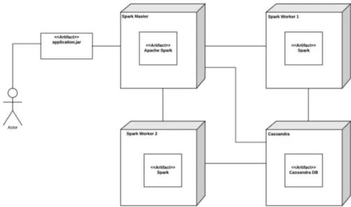
The running environment consists of 4 nodes. 3 nodes for Spark and 1 node for Cassandra DB. All nodes have 2 cores and 4GB of RAM. The three nodes of Spark are 1 driver and 2 workers. The Operating system of all 4 nodes is Ubuntu 16.04. The version of installed Spark is 1.6.3 and for Cassandra DB is 3.9. Figure 3.2 is a deployment digram for the application.

Figure 3.2: deployment diagram of the Apache Spark application

3.2 Installing the local work environment

In order to communicate with the Apache Spark driver, we need to install specific soft-ware. Below is the installed software to create and configure the working environment. Prerequisites:

• Java 8 • Ubuntu

The installed software is: 1. Scala 2.10.6.

2. SBT 0.13.13 to create a jar file. 3. Eclipse for Java EE developers. 4. Scala IDE.

(11)

During the installation, we faced some obstacles due to the compatibility issue between the code that we got from the company and the newly installed software that we made during the installation steps. The code started its development in 2016. This has caused some issue during the creation of the working environment, such as:

• Spark 1.6.3 should be installed and not the current version (2.3.0). • Java 8 and not the current version (Java 9).

• We need to install Scala version 2.10.x and not the newer one. • The SBT version 0.13.13 is deprecated.

The most significant obstacle was with SBT because the older version had been depre-cated. Therefore, we needed to change some configuration parts in the application to make it compatible with the most recent versions. Due to our lack of expertise in these development environments for Spark+Cassandra applications (the initial setup was done by Netfective company in France), finding the parts to change to make the installation work with the new versions required significant effort. For instance, we needed to edit the code inside build.sbt file. These changes are as follows :

The original code snippet was:

1 mergeStrategy in assembly <<=(mergeStrategy in assembly) { ( old ) => 2 {

3 case PathList ("META−INF", xs@_∗)=>MergeStrategy.discard 4 case x =>MergeStrategy. first

5 } 6 }

Then we changed it to:

1

2 assemblyMergeStrategy in assembly := {

3 case PathList ("META−INF", xs@_∗)=>MergeStrategy.discard 4 case x =>MergeStrategy. first

5 }

After these modifications, the installation completed and I could communicate with the Spark server on the remote cluster. The remote cluster is composed of a Spark Master node, two worker nodes, and a server with a Cassandra database. It is located in Spain. To be able to successfully launch an application in the Spark server, we first need to send via ’scp’ command the .jar file containing the application to the Spark Master node, then we connect to the Master node via ’ssh’ command, and finally we execute the ’spark-submit’ command with the .jar as argument, which launches the Spark process for our .jar application

3.3 Time measurement techniques

We used four techniques to measure the required time that each operation consumes dur-ing the execution. Moreover, these methods increase our confidence in the results. 3.3.1 Linux time command

Precedes the command line that used to execute the JAR file by linux time command. This command is useful to determine the time required for a specific code to execute. When

(12)

the executing finishes, the command shows a timing statistics to the standard output [9]. These statistics consists of:

• Real: Is the elapsed wall-clock time between launching command and its comple-tion.

• User, is the time spent by the CPU in user-mode. • Sys, is the system CPU time in kernel-mode. 3.3.2 Spark UI

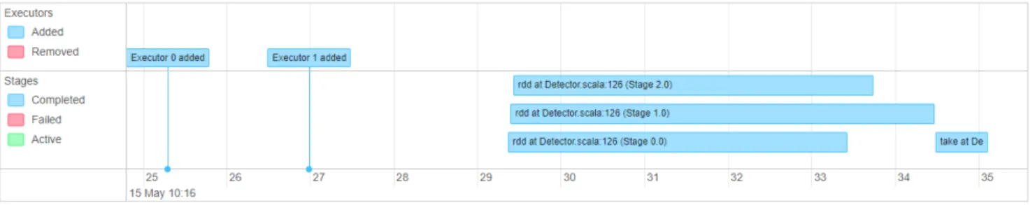
Every SparkContext has a web interface to monitor and display a useful information about the application [10], see Figure 4.4. This interfaced can be accessed by opening http : // < driver − node >: 4040 in a web browser.

3.3.3 Instrumenting the code: option 1 (Code 1)

We get a timestamp at the start and we get another timestamp when the code finished. Then the difference between these two time stamps will be the elapsed time for the code to execute. We do like this:

1 long start =System. currentTimeMillis () ; 2 ... some other code ...

3 long end= System. currentTimeMillis () ; 4 long total =end−start ;

Listing 1: Sample of Code 1 technique

3.3.4 Instrumenting the code: option 2 (Code 2)

Create a separate code that measures the time and neglect the creation of the database, while the previous method will not do that. In code snippet below, we can see an example of the rdd.map.f ilter.take(1) case:

1 def doRddMapFilterTake(inputRDD: DataFrame): Unit={ 2

3 time {

4 inputRDD

5 . rdd

6 . map(row=>(row. getString (0) , row. getString (1) , row. getString (2) , row. getString (3) ,

row. getString (4) , row. getString (5) , row. getString (6) , row. getString (7) , row. getString (8) , row.getDouble(9) , row. getString (10) , row. getString (11) , row.getDouble(12)) )

7 . filter ( tuple =>LocalDateTime.parse( tuple . _12). getYear ==LocalDateTime.parse( tuple .

_9) . getYear + 1)

8 . take (1)

9 } 10 }

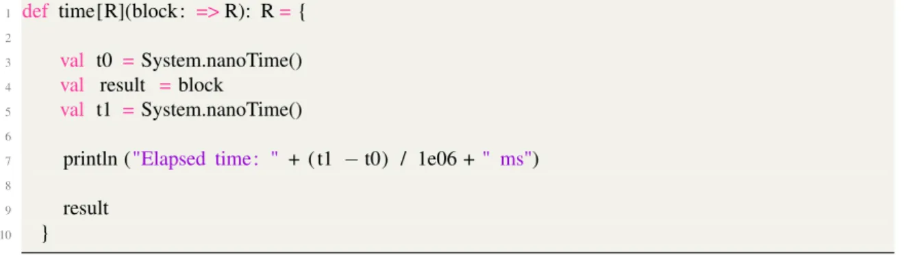
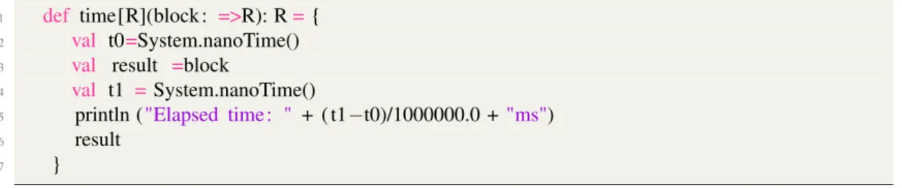
The method in code snippet above has the inputRDD database as an input parameter. The parameter is a Cassandra database of the Big Blu application. The method reads the input tuples (rdd), then map each row to a new dataset. After that, it executes the filter operation for each tuple. The declaration of time() method is shown below:

(13)

1 def time[R](block : =>R): R={ 2

3 val t0 =System.nanoTime()

4 val result = block

6

7 println ("Elapsed time : " + ( t1 − t0) / 1e06 +" ms") 8

9 result

10 }

The block input parameter is a block of code that measures the time for it. 3.4 PROS and CONS for each technique

The four techniques that we used to measure the time, is the tricky part of the measurement process because it returns different values of the same database. Table 3.1 shows the pros and cons for each method.

Method PROS CONS

Linux time command The method is simple and easy to use.

It relies on the specifications of the processor. For example number of cores, speed, performance, etc. Moreover, the Apache Spark is a cluster computing system which means that the Spark applications run in more than one mode and processes by executers (workers). And so the measured cpu time in the master node does not represent the actual consumed time to execute the application

Spark UI

This technique measures the time required for creating the RDD, (Resilient Distributed Datasets) which is a read-only data, inside the nodes. It also shows the amount of time the action operationconsumes to execute.\cite{SparkUI}

It does not show the required time for the transformation operations to execute. The visible parts are the rdd and the action operation only

Code 1 Straightforward and easy to use. Measures wall-clock time, that may affected by many factors like CPU performance Code 2 Not Straightforward

We have a full control over the output results. In addition, we can select the required

portion of code that we need to measure the time for.

Table 3.1: Time measurement methods PROS and CONS

After analysing and studying each approach, we could (mainly) adopt the Code 2 tech-niquein my discussions and analyses, due to the flexibility and the ability to have a control over the time measurements.

(14)

4 Performance Engineering - Measurements

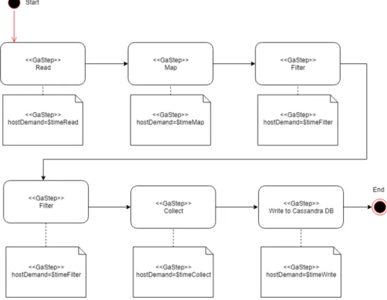
4.1 Activity Diagram

We extend the deployment digram explained previously (Figure 3.2) to visualize the ap-plication execution model. In Figure 4.3 we see that the apap-plication starts by reading from Cassandra database then do the map operation according to some conditions. After that, it executes two filters with some conditions like, age, income, etc. Then collect the results to finally write it to Cassandra.

For computing the performance of the whole activity diagram, it is necessary to know the values of $timeRead, $timeFilter, $timeFilter, $timeMap, $timeCollect and $timeWrite. And these values were not known. Therefore, during this thesis, we have done experiments to unveil these values. Moreover, our experiments give these previously unknown values as a function of the Size of the database; which will help the Performance Engineer to reuse our work to evaluate the activity diagram for the sizes of the databases he/she prefers.

Figure 4.3: The activity diagram of the application execution

4.2 Time measurement process

We followed a sequence of steps to perform the time measurement process.

1. Split the code into smaller code (cases) that includes each of the transformation operation as follows:

• Case 1: (.rdd + take (1) ) • Case 2: (.rdd + .map + take(1))

(15)

• Case 4: (.rdd + .map + .filter + filter + take(1)) • Case 5: (.rdd + .map + .filter + filter + collect()) • Case 6: (.rdd + .map + .filter + filter + collect + write)

2. Each Spark transformation will be followed by take(1) operation (which is an action operation that returns one tuple). The purpose of this additional action is to ensure that the precedent transformation operation actually executes.

3. We used the four techniques explained in previous section to measure the time. We found some similarity in the time measurement result in some cases that we will discuss it later.

4. Create a jar file by using sbt assembly command.

5. Copy the jar file to the Apache Spark remote cluster (located in Spain). 6. Execute the jar file in the Spark server with a small database.

7. Observe and record the average of the time measurements.

8. Repeat the previous steps, adding new transformation operation and followed by take(1)

9. After performing all the Spark operations, we redo the previous steps with a medium database.

Figure 4.4: Apache Spark UI

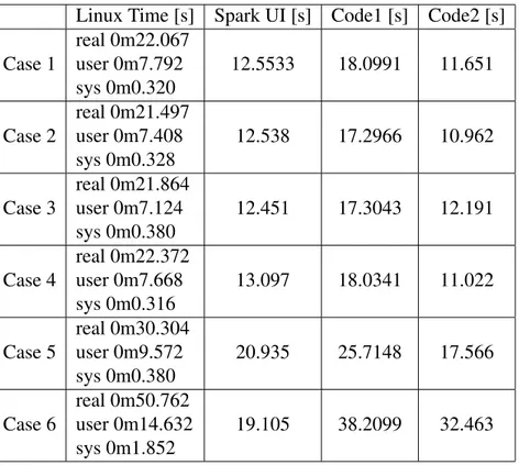
Table 4.2 shows the execution time measurement values for a small database with 85 tuples. While Table 4.3 shows the execution time measurement values for a medium database with 449439 tuples. We can see that Code1 values are higher than the rest of the measurement methods and that is because this method measures the wall-clock time. Furthermore, we can see that there is similarity in results between Spark UI and Code 2 for small and medium database except for the writing part in medium database.

4.3 Time measurement issue

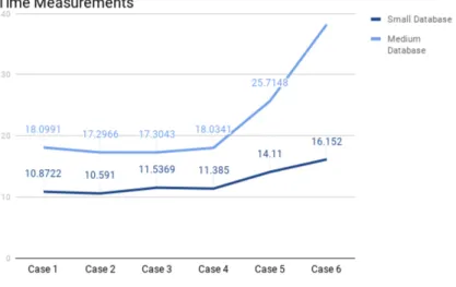
After performing several experiments with Big Blu workflow, we got a strong feeling that the execution time for the transformation operations does not affect the total time and the results from our experiments are not as we expected. Our expectation is that the time required to execute an operation should be proportional to the number of operations. In other words, the execution time for the operation should increase as the number of trans-formations increase. Figure 4.5 shows that Case1,2,3 and 4 have (almost) identical time

(16)

Linux Time [s] Spark UI [s] Code1 [s] Code2 [s] Case 1 real 0m18.771 user 0m8.056 sys 0m0.504 6.09 10.8722 6.086 Case 2 real 0m18.935 user 0m7.520 sys 0m0.332 6.074 10.591 6.207 Case 3 real 0m18.615 user 0m8.136 sys 0m0.572 6.487 11.5369 6.270 Case 4 real 0m18.730 user 0m7.880 sys 0m0.368 6.381 11.385 5.972 Case 5 real 0m18.905 user 0m9.660 sys 0m0.392 9.266 14.11 8.533 Case 6 real 0m28.650 user 0m9.432 sys 0m0.600 10.222 16.152 9.309

Table 4.2: The time measurements of the small database (85 tuples) Linux Time [s] Spark UI [s] Code1 [s] Code2 [s] Case 1 real 0m22.067 user 0m7.792 sys 0m0.320 12.5533 18.0991 11.651 Case 2 real 0m21.497 user 0m7.408 sys 0m0.328 12.538 17.2966 10.962 Case 3 real 0m21.864 user 0m7.124 sys 0m0.380 12.451 17.3043 12.191 Case 4 real 0m22.372 user 0m7.668 sys 0m0.316 13.097 18.0341 11.022 Case 5 real 0m30.304 user 0m9.572 sys 0m0.380 20.935 25.7148 17.566 Case 6 real 0m50.762 user 0m14.632 sys 0m1.852 19.105 38.2099 32.463

Table 4.3: The time measurements of the medium database (449439 tuples) measurements with different operations. For example, Case1 which has .rdd and take(1) , has a time measurement of 10.872s while Case4 that has .rdd, map, filter, filter and take(1) operations, has a time measurement of 11.385s and that is abnormal because these values are too similar.

(17)

Figure 4.5: A graph for the time measurements of small and medium db

To prove our expectation and to understand better the performance of Spark activities, we created an ad-hoc Spark application which can easily increment the amount of work carried out during Transformation activities, and we experimented with this application. We implemented a controlled experiment which consists of an application that includes a Map transformation whose amount of computation depends on the length of an array . Then creating a Map operation that consumes O(N*M) time being N the number of elements to map and M the size of the array passed as argument, so we can easily execute series of experiments with different sizes of arrays.

Concretely, the application consists of a function that is called with three parameters: • The first parameter can be "map", "reduce" or "mapreduce". The program will

do a Map transformation, a Reduce action or a Map transformation followed by a Reduce action. See listing 2.

• The second parameter is the length of an array whose elements are added during the Reduce.

• The third parameter is the length of an array that is traversed for each Map execu-tion.

1 time spark−submit −−class=[...] −−master=spark://10.10.10.108:7077 [ the path and name of the .

jar ] [ first parameter] [second parameter] [ third parameter]

Listing 2: A command to call the operation

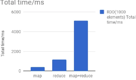
By performing these experiments, we will understand that the execution time required to perform a specific task, will rely on the amount of work done during this task. Table 4.4 and Table 4.5 are showing the result of executing the new code with 1000 and 10000 elements array respectively. Moreover, they also show the required time to perform a transformation operation (map) and the action operation (reduce) then a combination of (map and reduce) together. From the table, we can see that the transformation operation is almost immediate due to the lazy evaluation of Apache Spark.

For instance, under Creating list to reduce in Table 4.5, we can see that the time required for creating a list is close for each operation. While the Total time (which is the

(18)

required time for the operation to execute) is remarkably different for each operation. In other words, the Total time for the map operation (which is a transformation operation and it is the lazy part of Spark) is almost immediate, and that is because it will not execute until performing an action operation. Whereas the Total time of the reduce operation (which is an action operation) consumes time to execute.

Finally, the map+reduce operation consumes more time than map and reduce together. That is to say, map operation actually executes and it needs some time to finish the work different from the case when map executed alone without reduce. In other words, the reduceoperation performs the action on the mapped elements and thus it needs to wait until the map ends.

Similarly, for the Parallelizing list to reduce (copying the elements of the list to create datasets that divided into logical partitions that can be operated in parallel) column in 4.5, we can see that the time required for parallelizing a list almost the same for all opera-tions. While the Total time for executing the operation is significantly different for each operation.

Below are a snippets from the code that we used to perform the experiments. The first line of code snippet in listing 3 checks which method will be executed map, reduce or mapreduce. The second line will call doM apReduce method that has two parameters rddList (the second parameter in the called function) which is a parallelized list and spentT imeList (the third parameter in the called function) which is a an array to perform a work to do for the map operation. After that the method will print the result.

1 if ( args (0) =="mapreduce") {

2 val mappedReduced=doMapReduce(rddList, spentTimeList)

3 println (" Result of mapreduce is : " + mappedReduced +" and first element of itereated list is : " + spentTimeList (0) ) ;

4 }

Listing 3: Calling mapreduce method

In the code listing 4 below, the doM apReduce() method has two input parameters which is toSquare and dummy. The toSquare is our parallelized list and dummy is the array that is used to perform the map work. Each element of the toSquare RDD list will be mapped into a new squared element then the mapped list will be reduce by adding all elements to each other.

1 def doMapReduce(toSquare : RDD[Long], dummy : Array[Int]) : Long={ 2 println ("Doing MapReduce")

3 time{toSquare . map(x=>mapSpendTime(x,dummy)).reduce((a,b)=>a+b)} 4 }

Listing 4: Declaration of doM apReduce() method

The method mapSpendT ime() declared in code listing 5. This method has two param-eters; x and iter. The iter parameter is an array that is used to perform some work to do. While the x parameter is multiplied by itself and returned as long.

1 def mapSpendTime(x: Long, iter : Array[ Int ]) : Long={ 2 for(index <−0 until iter . size ){

3 iter (index)=iter (index)+1;

4 }

5 x∗x 6 }

(19)

The time() method, code listing 6 below, measures the elapsed time for the map and reduce operations to execute. Moreover, the method has a block parameter as an input. The block parameter is the block of code that will be measured. Finally, the elapsed time will be calculated and printed in ms.

1 def time[R](block : =>R): R={

2 val t0=System.nanoTime()

3 val result =block

5 println ("Elapsed time : " + ( t1−t0)/1000000.0 +"ms")

6 result

7 }

Listing 6: The declaration of time() method To create Table 4.4 we executed the following commands:

• To execute map() method:

1 time spark−submit −−class=. . . −−master=spark://10.10.10.108:7077 [ the path and name

of the . jar ] map 1000 10000000

• To execute reduce() method:

of the . jar ] reduce 1000 10000000

• To execute mapreduce() method:

of the . jar ] mapreduce 1000 10000000

RDD(1000 elements)

Operation Total time [ms] Creating list to reduce [ms] Parallelizing list to reduce [ms]

map 395.818841 23.521717 376.611462

reduce 1188.480588 35.429135 411.696702

map+reduce 5108.000853 28.912448 436.509436

Table 4.4: Shows the time measurements for 1000 RDD element And to create Table 4.5 we executed the following commands:

• To execute map() method:

of the . jar ] map 10000 10000000

• To execute reduce() method:

of the . jar ] reduce 10000 10000000

(20)

Figure 4.6: The required time to execute map, reduce and map+reduce with 1000 elements array

of the . jar ] mapreduce 10000 10000000

RDD(10000 elements)

Total time/ms Creating list to reduce Parallelizing list to reduce

map 386.306368 41.893611 363.359693

reduce 1766.784591 54.332705 337.945573

map+reduce 31274.85187 35.52478 316.192104

Table 4.5: Shows the time measurements for 10000 RDD element

Figure 4.7: The required time to execute map, reduce and map+reduce with 10000 ele-ments array

With these new results from the experiments, we proved that our expectation from our experiments is what we assumed from our common sense. The results obtained in these

(21)

experiments have provided calmed us down about the unexpected performance measure-ments of Transformation activities in the previous Big Blu case study. This experiment showed that Transformation activities are lazy but, when executed, require some compu-tation time that can be measured by instrumenting the code. It is worth noting that the amount of Scala instructions to execute during the Transformation was 1, 000 ∗ 106 _{= 10}9

for the experiment in Table 4.4 and 10, 000 ∗ 106 _{= 10}10 _{for the experiment in Table}

4.5. On the other hand, Big Blu executed 1 to 2 million Scala instructions when exper-imenting Transformations using the the medium database and just in the order of a few hundreds when using the small database. Therefore, we can conclude that the Transfor-mation time for BigBlu will be orders of magnitude lower than the time measured in this latter experiment with an ad-hoc application.

Due to the time needed to the distribution of tasks to parallelize and subsequent syn-chronisation in our BigBlu case study, the actual time required to execute the Transforma-tion activities is negligible with respect to the time required to execute the rest of activities, and thus also hardly measurable.

5 Performance Engineering - Observation and Analysis

According to the previous readings of the experiments, I observe the following:

• The time measurements for case 1, case 2, case 3 and case 4 are almost the same, which is unexpected.

• When we have the collect() operation (which is an action operation), we found that the time increases, as we expected.

• The last step is to write data to a new database. This operation takes more time than the other operations. We knew that writing the computed results by Spark to a database would consume a part of the execution time, but we did not know how much.

• The number of tuples in case 1 and case 2 are the same. In other words, the rdd operation will not affect the number of tuples because it performs read operation only. Similarly, map operation will only transform each element from one object into other.

• The execution time of the application grows with the size of the input database. We will study this correlation in next subsection in order to make predictions of future execution times.

Discussion:

• Case 1 and case 2 have the same time measurements because they use the same number of entries in their inputs. Moreover, map() operation is transforming the data from one type to another type. It works on each and every element of the RDD one by one to create a new RDD [11].

• The time required to execute and perform the operation depends on the Spark action more than Spark transformation. Due to the lazy behavior of Spark transformations [12]: 1) the transformation operation remembers the work to apply to the database without actually executing it, and 2) when it finally executes, it is not straightfor-ward at all to measure the time consumed by the Transformation part. We had

(22)

to include additional operations whose execution time is measured together with the Transformations, and then try to recognize the amount of time dedicated to the transformation. For this, we used the differences with other executions that were identical except for the lack of the transformation activity.

• As expected, time consumed depends on the size of the database.

• The execution time of the transformation operation (TT ransOpr) does not affect the

total time for this concrete case study. Spark UI does not show any time event for these operations either, see Figure 4.4. In addition, all the previous time measure-ments techniques that we have used so far, show that the values are almost identical with the first case which is the time measurement for the rdd operation (Trdd).

• Transformations may actually require significant time in the Spark workflow, as we explored with our ad-hoc additional experiments in Section 4.1, which helped us learn about the influence of much time-demanding transformations together with lazy operations.

5.1 Regression Study

According to the previous analyses and the collected time measurements, we come up with a formula where each operand is computed as a linear function that depends on the size of the input (i.e., the number of tuples in the Database). It can help the performance engineers to adopt a design decision in early iterations.

We used a linear regression formula Y = a + bX where Y is the single scalar response variable and X is the single scalar predictor variable. We observed that the resulted values from our experiment are non curvature values see Figure 1.13, which make us choose the linear regression in our analyses. In addition to its simplicity, the linear formula includes some useful statistics such as p-values for coefficients [13]. More about the regression analyses in the next subsection.

The formula:

TBigBlu(x) = Trdd(x) + Tmap(x) + Tf ilter1(x) + Tf ilter2(x) + Tcollect(x) + Twrite(x)

Trdd(x) = Ax + B Tmap(x) = Ax + B Tf ilter1(x) = Ax + B Tf ilter2(x) = Ax + B Tcollect(x) = Ax + B Twrite(x) = Ax + B

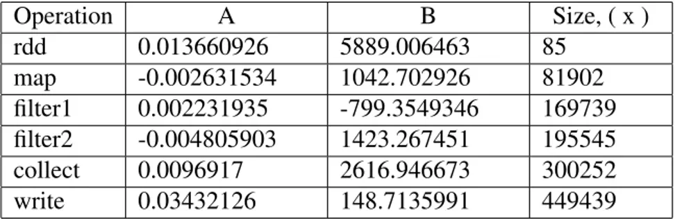
A and B are constants, x is the database size (number of tuples). To obtain A and B, we performed a regression analyses study over the measured execution times in Big Blu. Measurements ranged from a small database with 85 tuples to a database with half a million. Right column in Figure 5.6 presents the different sizes of inputs experimented. By using this study, we can find a correlation between the time measurements and the size of the database. Essentially, regression helps us to understand the behaviour of our measurement values and to create a formula that predicts the result of other size of the database for being used in performance tasks for the production system [14]. In Appendix A, Figures 1.10, 1.12, 1.14, 1.16, 1.18 and 1.20 show the results of the regression analysis

(23)

and Figures 1.13, 1.15, 1.17, 1.19 and 1.21 show the time plot of the regression study. The Aand B constants, shown in Table 5.6, are x variable 1 and intercept respectively under Coefficientscolumn. We used the Data Analysis tool of Microsoft Excel for this study.

Operation A B Size, ( x ) rdd 0.013660926 5889.006463 85 map -0.002631534 1042.702926 81902 filter1 0.002231935 -799.3549346 169739 filter2 -0.004805903 1423.267451 195545 collect 0.0096917 2616.946673 300252 write 0.03432126 148.7135991 449439

Table 5.6: Shows the values of A and B

5.1.1 Observations

A coefficient (X Variable) is called an independent variable, which shows the correlation between the input variables and the response (independent variable). In other words, it describes how the changes in inputs affect the response. The positive value means that the independent variable in proportional to the dependent variable. That is to say when the input variable increases the response increases also. In contrast, the negative sign means that there is a reverse relation between the dependent and independent variables. Table 5.6 shows that there are two negative values for map and filter2. In our case, these values should be positive because we expect that the independent variable related directly to the dependent variable. In other words, we expect that the output value (time measurement of the operation) should increase as the size of the database increase. We think that the server, sometimes, is busy doing some preparations for the task to execute. Moreover, it divides the work between nodes, creates RDDs and does undersign operation to complete the job [15].

Regarding the negative value in the B constant (intercept) for filter1, it means that the interception with Y axes happened in the negative direction. That is, for lower sizes of input, we measured that the Spark application executed faster having this operation filter1 than just skipping it, which is very unexpected. This behavior is also abnormal because of the same reasons discussed above. It is worth noting that all these odd values resided in the lazy and most difficult part to accurately measure, the transformation operations of Spark.

There is one more parameter which is essential in the regression study, the P-value. This value determines if the result is statistically significant or not. If the P-value is less than or equal to 0.05, that means the result is statistically significant [15]. In our case, we see that the P-value for the rdd and collect is less than 0.05, which means that there out result is statistically significant and there is a correlation between independent and dependent variables. While, in map, filter1, filter2 and write the P-value is higher than 0.05.

6 Performance Engineering-Validation and Discussion

This section validates our formula. We do the validation by using the formula to predict the performance of BigBlu with a larger database, and then compare the prediction with real performance measurement results.

(24)

Since the calibration of the values for the formula used databases of up to 449439 tu-ples, now, for validation, we use a database that is around double the previous size. There-fore, we created a database that contains 981947 tuples. We used the formula presented in previous section to predict the execution time of BigBlu using this large database. Middle column in Table 6.7 shows the results. We also created a database with these 981947 tuples and we measured the execution time using Code2 method. Right column in Table 6.7 shows the results.

Comparing the predicted and measured results, we noticed that the formula gave quite accurate predictions in most of the cases. Actually, three out the six measured steps give a error of only between 10% and 20%, which we take as very good prediction as we are using the formula for a size value much larger than the used values for its calibration.

However, we see that the formula has predicted slightly different in the Write oper-ation (last row in Table 6.7). The real execution has been much faster than predicted. We assume that something that we do not completely know executes during the Write operation to a Cassandra database, and so our model does not predict it accurately. For instance, the server could do some extra work under the hood to release the workers and deallocate the resources that were reserved for the Write operation, although the opera-tion has not completely finished in the remote database. These factors might cause the deviation between the real and measured value for the large database. We should look into the details of Write operation to give conclusions with confidence in this regard, but this detailed study of the concrete operation is out of the scope of this project work.

To finalize this section, we would like to graphically show the change in the execution time of our case study, part by part of its workflow, using as input three different databases: small (85 tuples), medium (449439 tuples), and large (981947 tuples). Figures 6.8 and 6.9 show these changes in the execution time. We can see that the type of execution time evolution for medium and large databases is quite hard to predict, and so we feel quite satisfied for being able to predict the execution time of the whole application and each of its subparts incurring in errors of only 10%-30%.

Operation Theoretical Time [ms] Experimental Time [ms] Error [%]

rdd+take 19303.31204 22638.47601 17.27 rdd+map+take 17761.98826 22507.17785 26.72 rdd+map+filter+take 19154.27548 22408.01959 16.98 rdd+map+filter+filter+take 15858.40086 21952.39084 38.42 rdd+map+filter+filter+collect 27992.08311 31665.05013 13.12 rdd+map+filter+filter+collect+write 61842.45483 45428.24549 26.54

(25)

Figure 6.8: The theoretical and experimental values of the formula

Linux Time [s] Spark UI [s] Code1 [s] Code2 [s] Case 1 real 0m37.742 user 0m7.888 sys 0m0.344 28.397 32.934 22638.47601 Case 2 real 0m36.419 user 0m7.780 sys 0m0.368 26.699 31.664 22507.17785 Case 3 real 0m36.018 user 0m7.772 sys 0m0.444 26.509 30.839 22408.01959 Case 4 real 0m35.631 user 0m7.572 sys 0m0.368 26.435 31.5876 21952.39084 Case 5 real 0m48.575 user 0m10.100 sys 0m0.396 38.994 44.1018 31665.05013 Case 6 real 1m8.982 user 0m14.896 sys 0m1.816 37.524531 56.469 45428.24549

(26)

(27)

7 Conclusion and Future work

Regarding objective two (O2), we experienced some obstacles and it was not as straight-forward as we expected. We observed that some versions of the infrastructure are depre-cated. Sometimes we need to install the old versions to be compatible with Apache Spark application. Thus, as we discussed in section 3.1, we needed to change some configura-tion parts to make it compatible with the applicaconfigura-tion. Although the lack of informaconfigura-tion regarding the Scala programming language and Spark, we studied the application and we tried to identify the relevant parameters. We observed that the Fraud Detection func-tionality of Big Blu application was fairly complicated. As we expected, and because of the lazy behaviour of the Apache Spark, we experienced some issues during the time measurements process as discussed in subsection 4.3. However, we could identify the parameters that we need to control and achieve our objectives. With respect to O6, we noticed that, in some cases, the obtained values from objectives 3 and 4 have some per-centage error which is lower than expected, such as in the case of writing to Cassandra database.

The result obtained by conducting the experiments in line with utilising a different kind of time measurements techniques with different size of databases shows some signif-icant aspects of Apache Spark lazy behaviour. Furthermore, by revealing the relationship between the total execution time required by the BigBlu system and each of the Spark ac-tion and Spark transformaac-tion operaac-tions, the performance engineers can take decisions in early design phases. Besides, they can predict the system performance before deploying the system in the production environment.

So far, our measurements and analysis indicate that the Bottleneck in BigBlu resides in the acquisition and writing of results (read and write operations), rather than in their processing. Therefore, we can tell BigBlu engineers that they do not need to worry (so far) about the performance of the internal transformations they develop because these computations are far from being the performance bottleneck.

For the future work, we need to investigate more about the Write operation to a Cas-sandra database. If we can measure the time required for the operations that are executing in parallel under the hood during the write operation, then we can have a more accurate formula. Moreover, during our time measurements, I found that there is a strange be-haviour that Apache spark behave which is if we have more than one action operation in the workflow, the first action operation consumes more time than the rest of the op-erations. In other words, if there is a (<some code>).count() operation and then when have a (<some code>).count() operation then we observed that the first one needs more time than the second operation. I started to investigate and I got some time measurement values. I also could change some parameters like separating each array that is used with each operation and I got the same behaviour. I need to go further and to create more jobs to be executed, change more parameters like work with different kinds of operations and measure the time and resources consumed.

(28)

References

[1] S. Salloum, R. Dautov, X. Chen, P. X. Peng, and J. Z. Huang, “Big data analytics on apache spark,” International Journal of Data Science and Analytics, vol. 1, no. 3-4, pp. 145–164, 2016.

[2] (2016) Demonstrators implementation plan. [Online].

Avail-able: http://wp.doc.ic.ac.uk/dice-h2020/wp-content/uploads/sites/75/2016/06/D6. 1-Demonstrators-implementation-plan.pdf

[3] “Spark overview.” [Online]. Available: https://spark.apache.org/docs/latest/

[4] D. Team. (2016) Spark rdd operations transformation and ac-tion with example. [Online]. Available: https://data-flair.training/blogs/ spark-rdd-operations-transformations-actions/

[5] P. Torres, J.-W. van Wingerden, and M. Verhaegen, “Hierarchical subspace identifi-cation of directed acyclic graphs,” International Journal of Control, vol. 88, no. 1, pp. 123–137, 2015.

[6] D. Perez-Palacin, Y. Ridene, and J. Merseguer, “Quality assessment in devops: Automated analysis of a tax fraud detection system,” in Proceedings of the 8th ACM/SPEC on International Conference on Performance Engineering Companion. ACM, 2017, pp. 133–138.

[7] “Dice: Devops for big data.” [Online]. Available: http://www.dice-h2020.eu/ [8] M. O’Sullivan. (2013) Barc big data survey: Lack of experts and know-how a

main obstacle to monetizing big data. [Online]. Available: https://www.teradata.de/ Press-Releases/2013/BARC-Big-Data-Survey-Lack-of-Experts-and-Kno

[9] “Linux time command information and examples,” Apr 2017. [Online]. Available: https://www.computerhope.com/unix/utime.htm

[10] “Monitoring and instrumentation.” [Online]. Available: https://spark.apache.org/ docs/latest/monitoring.html

[11] “Comparison between spark map and flatmap,” Jan 2018. [Online]. Available: https://techvidvan.com/tutorials/spark-map-and-flatmap-comparison/

[12] “Lazy evaluation in apache spark – a quick guide,” Jun 2017. [Online]. Available: https://data-flair.training/blogs/apache-spark-lazy-evaluation/

[13] J. Frost, “How to choose between linear and nonlinear regres-sion,” Oct 2018. [Online]. Available: http://statisticsbyjim.com/regression/ choose-linear-nonlinear-regression/

[14] N. R. Draper and H. Smith, Applied regression analysis. John Wiley & Sons, 2014, vol. 326.

[15] J. Frost, “Predictor variables,” Feb 2017. [Online]. Available: http://statisticsbyjim. com/glossary/predictor-variables/

(29)

A

Appendix

A.1 Regression study figures

Figure 1.10: Regression study of rdd

Figure 1.11: Time distribution of rdd

(30)

Figure 1.13: Time distribution of map

Figure 1.14: Regression study of filter1

Figure 1.15: Time distribution of filter1

(31)

Figure 1.17: Time distribution of filter2

Figure 1.18: Regression study of collect

Figure 1.19: Time distribution of collect

(32)

(33)

A.2 List of acronyms used

RDD Resilient Distributed Dataset DAG Directed Acyclic Graph VAT The Value Added Tax

IDE Integrated Development Environment SBT Scala Build Tool

UI User Interface

DB Database

A.3 Key words definition

Big Blu A Data Intensive Application in the field of Big Data Big Data A term used to refer to data sets that are too large or

com-plex for traditional data-processing application software to adequately deal with

Apache Spark Is an open source parallel processing framework for run-ning large-scale data analytics applications across clustered computers

DICE H2020 Open source framework for quality-aware DevOps for Big Data applications

Cassandra A highly scalable, high-performance distributed database designed to handle large amounts of data across many com-modity servers, providing high availability with no single point of failure