Linköping University Post Print
A Framework for Simulation of Surrounding
Vehicles in Driving Simulators
Johan Janson Olstam, Jan Lundgren, Mikael Adlers and Pontus Matstoms
N.B.: When citing this work, cite the original article.
© ACM, (2008). This is the author's version of the work. It is posted here by permission of
ACM for your personal use. Not for redistribution. The definitive version is:
Johan Janson Olstam, Jan Lundgren, Mikael Adlers and Pontus Matstoms, A Framework for
Simulation of Surrounding Vehicles in Driving Simulators, 2008, ACM Transactions on
Modeling and Computer Simulation, (18), 3, .
http://dx.doi.org/10.1145/1371574.1371575
Copyright: Association for Computing Machinery
http://www.acm.org/
Postprint available at: Linköping University Electronic Press
http://urn.kb.se/resolve?urn=urn:nbn:se:liu:diva-17449
A Framework for Simulation of Surrounding
Vehicles in Driving Simulators
Johan Janson Olstam∗†‡ Jan Lundgren†§ Mikael Adlers ∗¶
Pontus Matstoms∗k
Abstract
This article describes a framework for generation and simulation of surrounding vehicles in a driving simulator. The proposed frame-work generates a traffic stream, corresponding to a given target flow and simulates realistic interactions between vehicles. The framework is based on an approach in which only a limited area around the driving simulator vehicle is simulated. This closest neighborhood is divided into one inner area and two outer areas. Vehicles in the inner area are simulated according to a microscopic simulation model including advanced submodels for driving behav-ior while vehicles in the outer areas are updated according to a less time-consuming mesoscopic simulation model. The presented work includes a new framework for generating and simulating ve-hicles within a moving area. It also includes the development of an enhanced model for overtakings and a simple mesoscopic traf-fic model. The framework has been validated on the number of vehicles that catch up with the driving simulator vehicle and vice versa. The agreement is good for active and passive catch-ups on rural roads and for passive catch-ups on freeways, but less good for active catch-ups on freeways. The reason for this seems to be deficiencies in the utilized lane-changing model. It has been veri-fied that the framework is able to achieve the target flow and that
∗Swedish National Road and Transport Research Institute (VTI), Address: VTI,
SE-581 95 Link¨oping, Sweden
†Link¨oping University, Department of Science and Technology (ITN), Address:
SE-601 74 Norrk¨oping, Sweden
‡E-mail: johan.janson.olstam@vti.se
§E-mail: jan.lundgren@itn.liu.se
¶E-mail: mikael.adlers@vti.se
there is a gain in computational time of using the outer areas. The framework has also been tested within the VTI Driving simulator III.
1
Introduction
Many traffic accidents are caused by failures in the interaction between the driver, the vehicle, and the traffic system. Thus, knowledge about these interactions is essential and this is especially true nowadays since the number of driving related interactions is increasing. Today drivers also interact with different intelligent transportation systems (ITS), ad-vanced driver assistance systems (ADAS), in-vehicle information sys-tems (IVIS), and NOMAD devices such as mobile phones, personal dig-ital assistants, and portable computers. These technical systems influ-ence drivers’ behavior and their ability to drive a vehicle.
To get knowledge on how these kinds of systems influence drivers, researchers conduct behavioral studies and experiments, which either can be conducted in the real traffic system, on a test track, or in a driving simulator. The real world is of course the most realistic environ-ment, but it can be unpredictable regarding, for instance, weather, road, and traffic, conditions. It is therefore often hard to design real world experiments from which it is possible to draw statistically significant conclusions. Some experiments are also too dangerous or impossible to conduct due to ethical reasons. Test tracks offer a safer environment and the possibility of giving test drivers more equivalent conditions, but they lack realism. Driving simulators on the other hand offer a quite realistic environment in which test conditions can be controlled and varied in a safe way.
Driving simulators are used to conduct experiments in many differ-ent areas. Examples include alcohol, medicines and drugs, driving with disabilities, human-machine interaction, fatigue, road design, and ve-hicle design. A driving simulator is designed to imitate driving a real vehicle. The driver interface an be realized with a real vehicle cabin or only a seat with a steering wheel and pedals, and anything in be-tween. The surroundings are presented for the driver on a screen. It is important that the performance of the simulator vehicle, the visual representation, and the behavior of surrounding objects be as realistic as possible. For example, it is important that the ambient vehicles be-have in a realistic and trustworthy way. In this article we present a
traffic simulation framework that is able to generate and simulate these surrounding vehicles.
Microscopic simulation of traffic is one possibility for simulating these ambient vehicles. Micro-simulation has become a very popular and use-ful tool in studies of traffic systems. Micro-simulation models are time discrete models which simulate individual vehicle/driver units. The be-havior of vehicles/drivers and the interaction between those are simu-lated using different submodels for car-following, lane-changing, speed adaptation, and so on. The submodels use the current road and traffic situation as inputs and generate individual driver decisions regarding, for example, acceleration and preferred lane.
An important difference between simulation of surrounding vehicles for a driving simulator and traditional applications of traffic simulation is that one of the vehicles is driven by a human being. This puts additional demands on the modeling of vehicle movements since it is the actual behavior of the simulated vehicles that is the primary output. Most traffic simulation models are designed for generating correct outputs at a macroscopic level, for example, average speeds or queue lengths. The models often include assumptions and simplifications that do not affect the model validity at the macro level but sometimes affect the validity at the micro level. One typical example is the modeling of lane-changing movements. In most simulation models vehicles change lanes instantaneously. This is not very realistic from a micro-perspective, but does not affect macro measurements appreciably.
One approach for the simulation of the surrounding vehicles is to use available commercial micro traffic simulation tools. Some trials to use software packages such as AIMSUN (Barcel´o and Casas, 2002) and VISSIM (PTV, 2003) to simulate surrounding vehicles in driving sim-ulators have been conducted; see for example Ciuffo et al. (2007) and Jenkins (2004). One problem with using commercial programs is that they simulate a specified geographic area, for example, a part of a city or a road. Because of this, very large areas and thereby many vehicles, have to be simulated when running long driving simulator experiments (1-2 hours driving). For example, one-hour experiment at a traffic flow of 1000 vehicles/h will require that on average, 1000 vehicles per time step have to be updated. Another problem is that many of the pro-grams do not fulfill the additional demands on the modeling of vehicle movements we mentioned. A third drawback is that most commercial programs are not able to simulate rural roads with oncoming traffic, or
that the modeling of such roads is not detailed enough for this kind of application.
Another approach is to develop models specialized for the application of simulation of surrounding vehicles in driving simulators. Three of the most wellknown models following this approach are the ARCHISIM model (El hadouaj and Espi´e, 2002; Espi´e, 1995), the NADS model (Ahmad and Papelis, 2001), and the DRIVERSIM model (Wright, 2000). Research in this area has to a large extent been focused on decision making modeling concepts, for example the development of Hierarchical Concurrent State Machines (HCSM) (Cremer et al., 1995), which are used in the NADS model, the eco-resolution principle, which is used in the ARCHISIM model (Espi´e, 1999) and fuzzy logic modeling, which is used in the DRIVERSIM model (Wright, 2000). Focus has also to a large extent been limited to simulation of freeways. There has been little focus on modeling of rural roads and on algorithms for generation of realistic traffic streams.
In this article we present a framework for simulation and genera-tion of surrounding vehicles in a driving simulator. We present a traffic generation model that is able to generate realistic traffic streams: traf-fic streams with statistically correct time headway distributions. We also present both microscopic and mesoscopic1traffic simulation models which, can be used to simulate the surrounding vehicles close and far away from the simulator vehicle, respectively. The aim has been to base, as extensively as possible, the submodels for driving behavior on already developed models.
We only consider freeways with two lanes in each direction and with-out ramps, and rural roads with oncoming traffic but withwith-out intersec-tions.
The article is organized as follows: In Section 2 the developed sim-ulation framework is presented. Section 3 then continues with a more detailed description of the different components in the framework. First the microscopic traffic simulation model and its submodels for driving behavior are described. Then follows a description of the mesoscopic simulation model that is used to simulate vehicles further away from the driving simulator vehicle. After that follows a description of the model for the transition between the mesoscopic and the microscopic models.
1A mesoscopic traffic model simulates individual vehicles or packets of vehicles.
The difference compared to micro-simulation is that the vehicles’ behavior is described at an aggregate level, for example by using travel time functions.
The section ends with a description of the model for generation of new vehicles. The performed validation is presented in Section 4. Section 5 ends the article with some concluding remarks and suggestions for future research.
2
The simulation framework
When simulating traffic for a driving simulator, the area of interest is the closest neighborhood of the driving simulator vehicle. It is only within this neighborhood that vehicles have to be simulated. Similar approaches has been proposed both in Espi´e (1995) and in Bonakdarian et al. (1998). The area of interest moves with the same speed as the simulator vehicle and can be interpreted as a moving window, which is centered on the simulator vehicle. We have developed a simulation framework for generation and simulation of vehicles within such a mov-ing window (see Figure 1). The framework consists of four components: a microscopic traffic simulation model, a mesoscopic traffic simulation model, rules for the transition between the mesoscopic and the micro-scopic models, and a model for generation of new vehicles. This section describes how these four components are related to each other, and their basic functions. A more detailed description of each of these components is given in Section 3.
Driving direction of driving simulator Simulated area Candidate area Candidate area
Micro model Meso model
Meso model Transition model Generation model Generation model
Figure 1: Illustration of the simulation framework. The black vehicle is the driving simulator, the grey vehicles are simulated vehicles and the white vehicles are candidate vehicles.
The basic idea of the moving window is to avoid simulating vehicles several miles ahead of or behind the simulator vehicle, which is not effi-cient from a computational point of view. However, the window cannot be too small. First, the size of the window is constrained by the sight distance. The window must at least be as long as the sight distance, so that vehicles do not pop up in front of the simulator vehicle. Second, the window must be large enough to make the traffic realistic and to allow for speed changes of the simulator vehicle.
In order to get a wide enough window but at the same time limit the computational effort, the moving window is divided into one inner and two outer areas. The inner area is called the simulated area and the outer areas are called candidate areas. Vehicles traveling in the simulated area are simulated according to a microscopic simulation model that uses advanced submodels for car-following, overtaking and speed adaptation, and so on. It is important that the vehicles in the simulated area behave like real drivers, but the behavior of vehicles traveling further away from the simulator vehicle is less important. These vehicles, traveling in the candidate areas, are simulated according to a less time consuming mesoscopic model. When getting closer to the simulated area, these vehicles become candidates to move into the simulated area. In the approach proposed in Espi´e (1995) vehicles further away are simulated according to a macroscopic traffic model. The advantage with using a mesoscopic model is that it still simulates individual vehicles, but not a traffic stream as in a macroscopic model. This makes the transition of vehicles to and from the microscopic model more straightforward. At the end of the candidate areas, vehicles that travel out of the system are removed from the model and new vehicles are generated.
The candidate areas are in principle only necessary for traffic trav-eling in the same direction as the driving simulator vehicle. Oncoming vehicles far away in front of the simulator vehicle are assumed not to affect the driving simulator driver since they are not visible for the sim-ulator driver. Oncoming vehicles far behind the simsim-ulator vehicle may only affect the simulator driver in rare circumstances, for example by incidents that create congestion in the oncoming lane on rural roads.
3
Simulation and generation models
In order to be useful, the presented framework needs to be filled with suitable models for generation and simulation of vehicles. This section
presents the developed models for simulation and generation of vehicles starting with a description of how vehicles and drivers are represented.
3.1 Representation of vehicles and drivers
As in most micro-simulation models, vehicles and drivers are treated as vehicle–driver units. These vehicle–driver units are described by a set of driver or vehicle characteristics. Both the vehicle and the driver characteristics vary among different vehicle types. The vehicle types used are cars, buses, trucks, trucks with trailer with 3-4 axes, and trucks with trailer with 5 or more axes.
3.1.1 Vehicle parameters
The characteristics used to describe a vehicle are length, width, and the power to mass ratio, also called p–value. The p–value is the ratio between a vehicle’s power, available at the wheels, and its mass. For all vehicle types except cars, the p–value describes the vehicle’s maximum acceleration. For cars, the p–value describes the acceleration behavior at normal conditions. The average power/weight ratio for passenger cars is typically about 19 W/kg. A higher p–value can be used in special situations, for example in overtaking situations, in which car drivers tend to use higher acceleration rates. All vehicle parameters are assumed to be normally distributed within vehicles of a certain vehicle type.
3.1.2 Driver parameters
The characteristics used to describe the driver part of the vehicle–driver units are basic desired speed and desired time gap. The basic desired speed is the speed that a driver wants to travel at on a dry, straight, and empty road. This speed is assumed to be normally distributed for drivers driving a certain vehicle type. When assigning a desired speed to a vehicle, the driven vehicle’s acceleration capacity is checked. The vehicle has to be powerful enough to be driven at the desired speed. If that is not the case the vehicle–driver unit is assigned a new p–value.
The desired time gap is the time gap that a driver wants to keep from a preceding vehicle in car-following situations. The desired time gap is assumed to be lognormally distributed for drivers driving a certain vehicle type.
3.2 The microscopic model
The microscopic simulation model is based on established techniques for timedriven micro-simulation of road traffic. The model simulates sur-rounding traffic corresponding to a given target traffic flow and traffic composition. The model uses the simulator vehicle’s speed, position, and so on, as input, and generates the corresponding information about the surrounding vehicles as output. The simulation model follows a traditional time-discrete update approach. The update procedure has been divided into two parts. In the first part the speed and position are updated for all vehicles, and in the second part the behavior of the sim-ulated vehicles is updated: acceleration, lane-changing and overtaking decisions, and so on. In this way the update order of vehicles does not affect the result.
The submodels for vehicle movements and driving behavior used in this work are to a large extent based on submodels from the TPMA-model (Davidsson et al., 2002; Kosonen, 1999) and the VTISim TPMA-model (Brodin and Carlsson, 1986). These two simulation models are docu-mented in great detail and they have been well calibrated and validated for Swedish roads. However, some adjustments and further develop-ment have been necessary. In the following we give a brief description of the submodels for speed adaptation to the infrastructure, car-following, lane-changing, overtaking, oncoming avoidance, lateral movements, turn signals, and braking lights. The new model for behavior while overtak-ing will be given some extra focus. A more detailed description of the different submodels can be found in Janson Olstam (2005).
3.2.1 Infrastructure speed adaptation
The submodel for determining a vehicle’s desired speed at a section is based on the speed adaptation model used in VTISim (Brodin and Carlsson, 1986). This model describes speed adaptation on rural roads and has therefore been recalibrated for freeways; see Janson Olstam (2005) for details. The model starts from a median basic desired speed,
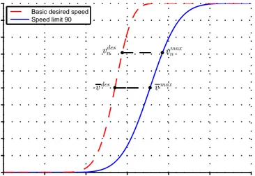
vmax. This median basic desired speed is then reduced with respect to speed limit, road width, and curvature to a median desired speed, vdes, for a specific section of a road. The desired speed for a vehicle n at a
road section is finally calculated as vndes = µ (vmaxn )Q− (1 − α) · µ (¯vmax)Q− ³ ¯ vdes ´Q¶¶1 Q , (1) where vmax
n is the basic desired speed of vehicle n and 0 ≤ α ≤ 1 is a vehicle type dependent parameter, equal to 0 for cars. The parameter Q is a transformation measure that depends on the reason for reduction: speed limit, road width, or curvature. Q = 1 implies a parallel shift of the basic desired speed distribution curve. Values of Q < 1 imply a counter clockwise rotation of the distribution curve around the median. This indicates that the desired speed of a driver with a high basic desired speed is more affected than a driver with a low basic desired speed. This rotation makes it possible to capture for example, that a vehicle with a high basic desired speed has to reduce its speed more in order to be able to drive through a sharp curve. An example of this rotation is given in Figure 2. This work used the calibrated values from Brodin and Carlsson (1986). 40 60 80 100 120 140 160 0 0.1 0.2 0.3 0.4 0.5 0.6 0.7 0.8 0.9 1
Cumulative desired speed distributions
Desired speed, [km/h] Basic desired speed
Speed limit 90 max v des n v vmaxn des v
Figure 2: Example of shift and rotation of a desired speed distribution.
3.2.2 Car-following
Research on car-following models started in the 1950s and several models have been presented since then. The most well known car-following
model is probably the GHR-model (Chandler et al., 1958), the Gipps model (Gipps, 1981), and the Wiedemann model (Wiedemann, 1974; Wiedemann and Reiter, 1992). For an overview on car-following models, see for example Brackstone and McDonald (1998) or Toledo (2007). The utilized car-following model is based on the HUTSIM/TPMA (Kosonen, 1999) model with some modifications. The car-following model uses three regimes: Free, Stable, and Forbidden. The regimes are defined by headways. The forbidden headway df is a function of the speed of the follower, vn, and the speed of the leader, vn−1; see Janson Olstam (2005) for details. The forbidden headway also depends on a driver-specific minimum desired time gap, an average normal deceleration rate, and a minimum distance between stationary vehicles. The stable regime is defined as the regime enclosed by the forbidden regime and the free regime. The length of the stable regime, ds, also depends on vn, vn−1, the minimum desired time gap, the average normal deceleration rate, and the minimum distance between stationary vehicles.
When a vehicle is in the free regime, xn−1−xn> df+ds(where xnis the position of vehicle n), the driver accelerates or decelerates in order to reach its desired speed. In the stable regime, df < xn−1− xn≤ df+ ds, the driver does not take any action—no acceleration or deceleration. If a vehicle enters the forbidden regime, xn−1 − xn ≤ df, the driver decelerates in order to reenter the stable regime.
For free accelerations, the acceleration model presented in Brodin and Carlsson (1986) is used, in which the free acceleration for vehicle n is calculated as
an= pvn
n − (CA)n· v 2
n− (CR1)n− (CR2)n· vn− g · i (xn) , (2) where pn is the p–value for vehicle n, CA, CR1, and CR2 are
vehicle-type-dependent air and rolling resistance coefficients, and g is the grav-itational acceleration constant. The function i(xn) represents the road incline at the position xn of vehicle n. For eventual decelerations in the free regime, vehicles are assumed to use an engine deceleration rate equal to the effect of rolling- and air-resistance and the gravitational acceleration, approximately 0.5 m/s2 when driving at 90 km/h. For decelerations in the forbidden regime, the deceleration rate depends on the ratio between the actual headway and the forbidden headway. For ratios close to 0, the driver brakes as hard as possible and for ratios close to 1 the driver uses the engine deceleration rate. In between these two
extremes the deceleration rate follows a piece-wise linear relationship; see Janson Olstam (2005) for details.
3.2.3 Lane-changing
There has recently been a focus on lane-changing models. The state-of-the-art in lane-changing models includes Gipps (1986), Hidas (2002, 2005) and Toledo et al. (2005, 2003). For an overview of lane changing models see Toledo (2007) or Janson Olstam (2005). The utilized lane-changing model is also based on the HUTSIM/TPMA (Kosonen, 1999) model, with some minor modifications; see Janson Olstam (2005) for details. In this model a pressure function is used for deciding whether or not a driver desires to change lane. The pressure is an estimation of the deceleration a vehicle needs to apply in order to avoid a collision with a vehicle in front. The decision to change to the left is based on the pressure to the closest vehicle in front in their own lane, Pf, and to the first vehicle in the left lane, Pf l, according to the rules presented in Figure 3. For lane changes to the right, the pressure from the vehicle behind in the left lane, Pb, and the pressure to the vehicle in front in the right lane, Pf r, is used. The parameters cland crare calibration param-eters, that control the willingness to change lane to the left and right, respectively. We have used the values suggested in Gutowski (2002).
Pfl Pf
Pb Pfr
Change to the left if: c Pl⋅ f >Pfl, cl∈
[ ]
0,1Change to the right if: cr⋅ >Pb Pfr, cr∈
[ ]
0,1Figure 3: Lane-changing logic based on the model presented in Kosonen (1999)
The pressure P between two vehicles is defined as P = ¡ vdes back− vfront ¢2 2 · s , (3) where vdes
backis the desired speed of the rearmost vehicle, vfront is the speed of the vehicle in front, and s is the distance between the two vehicles. In calculations of Pb, vbackdes has to be replaced with an estimate of the desired speed since the rearmost vehicle may be the driving simulator vehicle. In these situations the desired speed, vdes
back, has been estimated as the maximum of the current speed and the highest speed at which the vehicle was traveling at the last time it could have been considered free: not accelerating or decelerating.
If a driver desires to change lane, the possibility of a lane change is checked using a traditional gap-acceptance model; see Kosonen (1999) and Janson Olstam (2005) for details. If a lane change is both desirable and possible, the driver will initiate the lane change.
Observations of the simulation animation indicate that the simulated drivers change lane more frequently than one would expect and that the lane changing model lacks in anticipation of future traffic conditions in the different lanes. This causes the average travel speed to decrease more with increasing flow than the decrease seen in the speed–flow diagrams for two-lane freeways. Thus, the lane-changing model is not working as it should be and needs to be enhanced or replaced.
3.2.4 Overtaking
The state-of-the-art in overtaking and rural road models includes the TWOPAS model (Leiman et al., 1998), the TRARR model (Hoban et al., 1991), and the VTISim model (Brodin and Carlsson, 1986). The VTISim model is currently being further developed in the RuTSim model (Tapani, 2005a,b). For an overview of overtaking and rural road models see for example McLean (1989) or Tapani (2005a). The model used for overtaking on rural roads with oncoming traffic is based on the VTISim model (Brodin and Carlsson, 1986). This model states that a driver only accepts an overtaking opportunity if the following four conditions are fulfilled:
1. No overtaking restrictions. The road must be free of overtaking restrictions from the vehicle’s position and 300 meters ahead.
Re-strictions further away are assumed not to affect the overtaking decision.
2. Enough space. The estimated overtaking distance has to be shorter than the available gap, dgap, as defined in the following.
3. Ability to execute an overtaking. The estimated overtaking dis-tance must be shorter than 1000 meters. This constraint is used to avoid extremely long overtaking distances. An accelerated over-taking is only executed if the vehicle’s desired speed is higher than the preceding vehicle’s desired speed. The difference must at least be 0.5 m/s.
4. Willingness to execute an overtaking. An overtaking is only per-formed if the driver accepts the available gap.
The probability that a driver accepts a gap is determined by a stochastic probability function that is defined as
W (dgap) = e−A·e−k·dgap, (4) where dgap is the available gap, defined as:
min{distance to oncoming vehicle, distance to natural sight obstruction},
and A and k are constants that depend on type of overtaking {flying, accelerated}, type of sight limitation {oncoming vehicle, natural}, type and speed of vehicle being overtaken, and the current road width. Cal-ibrated values of A and k for Swedish road conditions is available in Carlsson (1993) and Janson Olstam (2005).
All drivers are assumed to have a higher desired speed during over-takings, currently set to an temporarily increase of 10 km/h. Car drivers are also assumed to use higher acceleration rates during overtakings, which is modeled as an increase in their p–value.
When overtaking, the overtaking vehicle must continuously reeval-uate the distance to the vehicle in the oncoming lane and the distance remaining for the overtaking. This was not included in the model presented in Brodin and Carlsson (1986). The overtaking model has therefore been enhanced with a more detailed modeling of overtakings including decision rules for abortion of overtakings. The developed
model for overtaking abortions is based on the assumption that a driver takes action if the time to collision, T T C, with the oncoming vehicle is less than the estimated time remaining for the overtaking. Thus, if
T T C + tsafety < tleft, where tsafety is a safety margin and tleft is the estimated time remaining for the overtaking. The time remaining is estimated as tleft = −vn− va n−1 n + sµ vn− vn−1 an ¶2 + 2∆d an + 0.5 · tchange, (5) where ∆d = xn−1− xn+ ln+ dmin. The parameter ln is the length of vehicle n, dmin is the critical lag gap for lane changes to the right, and
tchange is the time it takes to perform the lane change back to the normal lane. The reason for only adding half the time of a lane change is that this time is enough for clearing the oncoming lane and thereby avoiding a collision with an oncoming vehicle. The acceleration, an, is calculated according to Equation 2. In situations where T T C + tsafety < tleft, and the driver has not yet passed the lead vehicle, the driver is assumed to have aborted the overtaking. The driver then falls back and merges into the normal lane behind the lead vehicle. If the vehicle is side-by-side or has passed the lead vehicle, the driver instead increases the desired speed to a level needed to end the overtaking without colliding with the oncoming vehicle. If the vehicle’s p–value is too low in order to be able to accelerate to the new desired speed, checked via Equation 2, the vehicle is temporarily assigned a new power/mass value. However, if the p–value needed to drive at the new desired speed exceeds the maximum p–value for the current vehicle type, the driver aborts the overtaking and falls back in order to merge into the normal lane behind the vehicle that was to be overtaken.
3.2.5 Oncoming avoidance
Vehicles traveling on rural roads not only have to consider oncoming traffic when overtaking another vehicle, but also when oncoming vehicles overtake. On roads with wide shoulders, the natural reaction is to drive out into the shoulder if an oncoming overtaking vehicle is getting too close. On other roads vehicles decelerate and signal with the horn or using the high beam. If the situation becomes really critical, they try to drive out to the shoulder or the ditch in a last attempt to avoid a collision. In our model, drivers are assumed to go out onto the shoulder
on roads with wide shoulders if T T C < 2 · tchange+ tsafety, where tchange is the time for a lane change and tsafety is the added safety margin parameter. On roads without wide shoulders the driver instead signals with the high beam. However, if the T T C < 1.5 · tchange, the driver brakes and moves as far out on the shoulder as he or she can in order to avoid a collision, and lets the oncoming overtaking vehicle safely end or abort the overtaking.
3.2.6 Lateral movements
The vehicle’s lateral position, defined as the perpendicular distance to the center line of the road, is assumed only to change as a result of a change of lane. During a change of lane two different approaches for modeling the lateral movements have been tested. In the first, the vehi-cle’s lane-changing movement is assumed to follow a sine curve. In the second alternative, the movement follows a function that uses a second order polynomial in the beginning and at the end of the movement, and a linear relationship in between. Both approaches look quite realistic on freeways, where the lane-changing movements are made over quite a long period of time, about 4–6 seconds according to measurements presented in Liu and Salvucci (2002). However, on rural roads lane-changing move-ments are sometimes executed during a much shorter time, for instance during evasive maneuvers or when aborting an overtaking. It seems that neither of the two functions correctly represents lateral movements for quick lane changes. Another drawback is that these functions assume that all lane changes that are started, are completed. The functions cannot model the lateral movements when a driver decides to abort an ongoing lane-change. In order to overcome these drawbacks a more ad-vanced steering model is needed, perhaps a model similar to the one presented in Salvucci et al. (2001), or a control theory based model. 3.2.7 Turn signals and brake lights
In ordinary traffic simulations there is no need for simulating occurrences like the use of turn signals or brake lights since all vehicle actions are known within the model. However, when simulating traffic for a driving simulator it is important to model both turn signals and brake lights, otherwise such signals will not be visible for the simulator driver. Brake lights have in this work been assumed to be on when using deceleration rates higher than an engine deceleration rate, assumed to be 0.5 m/s2.
Drivers are assumed to use the turning lights with some probability, which differs between lane changes to the right and left and between freeways and rural roads. When driving on freeways, drivers are for instance assumed to use the left turn signal more often than the right.
3.3 The mesoscopic model
The mesoscopic model that is used to simulate vehicles within the can-didate areas must simulate individual vehicles and not packages of ve-hicles, which is an approach used in for example the mesoscopic model CONTRAM (Taylor, 2003). The model must also assign each vehicle an individual speed, not an average speed, as in several mesoscopic models; see for example the DYNASMART model (Jayakrishnan et al., 1994) or the MEZZO model (Burghout, 2004).
In an earlier version of the simulation framework the candidate ve-hicles were assumed to drive at their desired speed, (Janson Olstam, 2003; Janson Olstam and Simonsson, 2003). This worked properly for low traffic flows on freeways. However, on rural roads and at higher flows on freeways the candidate vehicles traveled too fast, which resulted in a quite empty candidate area in front of the simulator vehicle and con-gestion in the candidate area behind the simulator vehicle.
The developed mesoscopic model is based on the representative speed–flow relationships for Swedish roads presented in SRA (2001). These speed–flow relationships vary with road type, vehicle type, speed limit, number of lanes, road width, and sight class2 However, in the model not all dependent variables are used. The speed–flow relationship for cars is for instance used for all vehicle types and on rural roads the relationships for the best sight class (class 1) is used irrespective of the sight class of the simulated road. The relationships in the model depend on the road type, road width and the speed limit. The speed of vehicle
n is calculated as vn= µ f (q)Q+ µ³ vdesn ´Q − f (0)Q ¶¶1/Q , (6) where vdes
n is the desired speed of vehicle n, q is the traffic flow, and
f (q) is the average travel speed at a traffic flow of q vehicles/h. The
2The sight class is used in SRA (2001) for classification of the sight distance
conditions along a road, more or less a classification of the overtaking possibilities along a road.
parameter Q controls the rotation of the speed distribution curve. Values of Q < 1 imply that a vehicle with a high basic desired speed reduces its speed more than vehicles with a lower basic desired speed. Two different approaches have been tested, namely with or without rotation. In the case without rotation, Q = 1, vehicles will be able to drive as much faster or slower than the average speed than they do at free flow conditions.
Q = −0.2 has been chosen for the case with rotation. This is the value
used for speed adaptation to speed limits in the speed adaptation model presented in Brodin and Carlsson (1986). The model seems to perform well at both values of Q, but a value of Q < 1 appears to be more realistic, since deviations in speed generally are higher under free flow conditions than under congested conditions. Further calibration and evaluation is needed before a recommendation can be made.
Apart from the reduction of speed according to Equation 6, the can-didate vehicles travel unconstrained with regard to surrounding traffic. When a candidate vehicle catches up with another candidate vehicle it can always overtake the preceding vehicle without any loss in time. This can be interpreted as if every vehicle is driving in a separate lane, which is illustrated by the multiple lanes in the simulator vehicle direction in Figure 1.
3.4 Transition between the meso and the micro models
A candidate vehicle that reaches boundary of the simulated area, is allowed to travel into the simulated area only if there is a sufficient distance to the first vehicle in the simulated area. The rules for checking this differ between the two boundaries.
For vehicles in the driving simulator vehicle’s direction that want to enter the simulated area from the candidate area behind the simulator vehicle, the car-following model is used to deduce whether it can do so or not. The same applies for oncoming vehicles that want to enter the simulated area from the candidate area in front of the simulator vehicle. The vehicle is allowed to enter the simulated area if it can do so without decelerating, when the car-following model returns a non-negative accel-eration. If this is not the case, the vehicle adopts the acceleration given by the car-following model but the position is locked at the edge between the candidate area and the simulated area. This means that the vehi-cle’s position will be calculated using the speed of the window instead of using the vehicle’s own speed, and that the vehicle consequently will
move a shorter distance than its speed implies. The vehicle gets a new opportunity to pass into the simulated area in the next time step. While waiting for a sufficient gap, the candidate vehicle adjusts its speed in or-der to avoid rapid deceleration when entering the simulated area. There is also a minimum gap criterion, that the gap to the front vehicle must at least be larger than a minimum-distance-between-stationary-vehicles-parameter. Vehicles that are waiting at the boundary are treated as any other candidate vehicle but with the exception that their position increment may be restricted if they would pass into the simulated area without fulfilling the entering constraints. The vehicles at the boundary, as well as the other candidate vehicles, can overtake each other without any time delay. If there are several vehicles waiting at the boundary, the vehicle that first fulfills the entering constraints will be allowed to pass into the simulated area. This sometimes implies that this vehicle will overtake other candidate vehicles that are waiting at the boundary. When a vehicle is allowed to enter the simulated area, the calculation of its position will return to being based on its real speed instead of the speed of the boundary. In the freeway environment cars are also given the possibility of entering the simulated area in the left lane. In this case, a car is allowed to enter the simulated area if the lane changing model suggests a lane change to the left lane and if the car-following model returns a non-negative acceleration.
A similar approach is used for the transition of vehicles from the can-didate area in front of the simulator vehicle to the simulated area. The simulated vehicle closest to the candidate area treats the first vehicle in the candidate area as any other simulated vehicle. Thus, it uses the car-following model to adjust the speed and the lane-changing or overtaking model in order to decide whether it should try to overtake the candi-date vehicle. This is similar to the approach used in the other candicandi-date area, but instead of applying the car-following model on the candidate vehicle it is here applied on the following vehicle in the simulated area. Consequently, the candidate vehicle at the boundary is allowed to enter the simulated area if its entering does not imply a deceleration for the first vehicle in the simulated area.
There are no rules for the transition from the simulated area to ei-ther of the candidate areas. If a vehicle in the simulated area reaches the boundary of the simulated area, it will directly enter the candidate area and become a candidate vehicle. If the boundary behind the driving sim-ulator vehicle catches-up with a slower simulated vehicle, the simulated
vehicle will immediately become a candidate vehicle and any candidate vehicles waiting at the boundary will thereby overtake this vehicle with-out any time delay. It sometimes happens that a simulated vehicle who wants to drive at only a slightly lower speed than the driving simulator vehicle, hinders the entering of candidate vehicles from the candidate area behind the simulator vehicle for quite a long time. In order to avoid this, vehicles that are closer than 100 meters from this boundary and that have a desired speed lower than the simulator vehicle’s speed are directly moved to the candidate area behind the simulator vehicle.
3.5 Generation of new vehicles
Vehicles traveling much slower or faster than the simulator vehicle will travel out of the simulated area, into the candidate areas and finally out of the system. Thus, the system will become empty if no new vehicles are generated. Since our model does not include intersections or ramps, all new vehicles are generated at the edges of the window; see Figure 1. As the edges always move with the speed of the simulator vehicle, new vehicles cannot be generated in the same way as in ordinary traffic sim-ulation models, where new vehicles are generated at the geographical places that define an origin in the simulated network. Oncoming vehi-cles can, however, be generated almost in the same way as in ordinary simulation models. The difference is that the arrival time for an entering vehicle does not only depend on its own speed and headway but also on the speed of the simulator vehicle.
In the driving direction of the simulator vehicle, new vehicles are generated both behind and in front of the simulator. The generation process differs from generation approaches used in ordinary simulation models. For instance, when generating new vehicles at the edge behind the simulator vehicle it is only interesting to generate vehicles traveling faster than the simulator vehicle. Vehicles driving slower than the sim-ulator vehicle will never catch up with the edge between the candidate area and the simulated area. The opposite holds for the edge in front of the simulator vehicle, where there is no need to generate vehicles that drive faster than the simulator vehicle.
If only generating faster vehicles behind and slower vehicles in front of the simulator vehicle, the calculation of the vehicles’ arrival times cannot be done in the usual way. In ordinary traffic simulation models, vehicle arrival time is drawn from a time headway distribution. The
av-erage time headway between arriving vehicles is calculated as the inverse of the traffic flow. If the arrival time between faster vehicles generated behind the simulator vehicle were calculated like this, the average dis-tance between them would be equal to the average disdis-tance between vehicles. Since the vehicles generated behind the simulator vehicle form a subgroup of the total population of vehicles moving faster than the driving simulator vehicle, the actual average distance between vehicles in this subgroup is longer than the average distance between vehicles. If this is ignored, new vehicles will be generated with a higher frequency compared to reality, which results in a traffic composition that differs from the specified one. In order to deal with this problem a new gen-eration algorithm has been developed. This algorithm generates a new vehicle and calculates a reasonable time to arrival for the generated ve-hicle. For generation of a new vehicle behind the simulator vehicle, the algorithm works as follows:
1. Set i = 1.
2. Generate a new vehicle with a desired speed, vdes
i , and time head-way, ∆ti, to the vehicle in front of it.
3. Calculate the vehicle’s speed, vi, given its desired speed and the traffic flow, according to the mesoscopic model; see Equation 6. 4. If the speed is lower than the simulator vehicle’s present speed:
increase i and go to step 2, otherwise let n = i. 5. Calculate the time to arrival as
∆T = n P i=1 (∆ti· vi) vn− vDS ,
where vDS is the present speed of the simulator vehicle. 6. Discard all vehicles except the last generated.
7. When the simulation time has reached the time of arrival, add the generated vehicle to the relevant candidate area and rerun the algorithm to generate a new vehicle.
On rural roads the time headways ∆ti are drawn from an exponen-tial distribution. On freeways the time headways are instead assumed to
follow the time headway distribution developed in the HUTSIM/TPMA model (Blad, 2002), which has been specially developed for time head-ways on Swedish freehead-ways. At the edge in front of the simulator vehicle, new vehicles are generated according to a corresponding algorithm. The stop criterion is then a vehicle with a speed lower than the simulator vehicle’s present speed.
There is a risk that the algorithm gets stuck when for example trying to generate faster vehicles when the simulator vehicle is driving very fast. In order to avoid that and to limit the computational effort, new vehicles are only generated behind the simulator vehicle when it is traveling slower than the highest speed in the current desired speed distribution, and analogously for the edge in front of the simulator vehicle. For the same reason the number of tries at each time step has been restricted, currently to 10 presumptive new vehicles per time step: n ≤ 10.
In order to avoid too long time to arrivals, the speed of the generated vehicle, vn, must differ by at least 5 % from the simulator vehicle’s speed,
vDS. If the speed lies within this range, vDS < vn ≤ 1.05 · vDS for the edge behind the simulator vehicle and 0.95·vDS < vn≤ vDS for the edge in front, a speed equal to 1.05 · vDS, respectively 0.95 · vDS is instead used in the calculations of the arrival time.
Vehicles in the oncoming direction on rural roads are generated ac-cording to the vehicle platoon generation model presented in Brodin and Carlsson (1986). For an oncoming vehicle on freeways the HUT-SIM/TPMA model is used (Blad, 2002).
4
Validation
The aim of the developed simulation framework is to create realistic traffic situations around the simulator driver by coordinating different models for generation and simulation of vehicles. We have in this ar-ticle validated the framework by looking at the number of overtakings or catch-ups that the simulator vehicle experiences. The number of catch-ups is affected by all components in the framework. The gener-ation model has to generate the correct number of vehicles and with the correct characteristics; the rules for speed choices, lane changing, overtaking, and so on, in the micro and meso models have to be cor-rect; and the transition model has to let the correct number of vehicles into the simulated area from the candidate areas. In addition to this, we have compared the output flow from the simulation model with the
input target flow. We have also estimated the computational savings of using the candidate areas.
The primary output of the developed simulation framework is the behavior of the simulated vehicles in the simulated area; thus the pri-mary output is at a microscopic level and not at a macroscopic level, as is the case for most applications of traffic simulation. The overall objective for our application is that the simulator drivers experience the surrounding vehicles’ behaviors as realistic. If this is not the case the simulator drivers might behave differently than they would if they were driving a real car. However, the focus in this article is the simulation framework and not the submodels for driver behavior. We have there-fore, at this point, not done any validation of the actual driving behavior that the micro-simulation model generates. We have instead performed a small driving simulator study with the aim of getting a hint of how well the submodels for driving behavior describe real driving.
The section starts with a presentation of the study of overtaking rates of the driving simulator vehicle. It then continues with a comparison of target and obtained flows followed by a comparison of computational time when running the framework with or without the candidate ar-eas. The section ends with a description and results from the driving simulator experiment.
4.1 Overtaking rates
An important aspect relative to the observed realism, is the number of vehicles that catch up with the driving simulator vehicle and the num-ber of vehicles that the simulator driver catches up with. When driving at a certain speed you may not be able to say whether the number of vehicles that overtake you is comparable to the number when driving on a real road, but you certainly react if the proportion between vehicles that catch up with you (passive catch-ups) and the ones you catch up with (active catch-ups) is not realistic. We have compared active and passive catch-ups generated by the model with an analytical expression for estimating the number of catch-ups of a floating car, originally pre-sented in Carlsson (1995). The number of passive catch-ups is estimated as Up= qL ∞ Z v0 µ 1 v0 − 1 v ¶ ft(v) dv, (7)
where q is the traffic flow, L is the length of the observed road section,
v0 is the speed of the studied vehicle, and ft(v) is the time mean speed3 distribution. The number of active catch-ups is calculated in a similar way. One of the underlying assumptions for these functions is that all vehicles can overtake each other without any time delay. The equations can thus be expected to give upper limits on the number of active and passive catch-ups.
The values from the model were generated by simulating the driving simulator vehicle in addition to simulating the surrounding vehicles. In the rural environment, active catch-ups were estimated as the sum of the number of active overtakings and the queue length in front of the simulator vehicle at the end of the simulation. The passive catch-ups were estimated in a similar way. In the freeway environment, active and passive catch-ups were measured as the number of vehicles that the driving simulator vehicle passed and the number of vehicles that passed the driving simulator vehicle, respectively. Simulations were conducted with varying desired speeds of the simulator vehicle and at varying traffic flows. For rural roads the simulated values correspond quite well to the analytical calculation; see the example with 400 vehicles/h in each direction in Figures 4a and 4b. However, the simulated number of active catch-ups on freeways seems to be too low; see the example with 1000 vehicles/h in Figure 4d. The simulated values of the number of catch-ups are generally smaller than the corresponding analytical values as is predicted, because the analytical expression is an upper limit. However, there are some values in Figure 4b that lie over the analytical expression. The reason for this is that the driving simulator vehicle in these cases was driving in quite long platoons—15–25 vehicles—at the end of the simulation.
We suspect that the reason for the deviation of active catch-ups on freeways is due to the deficiencies in the lane-changing model, stated in Section 3.2. The deficiencies in the lane-changing model cause the speed–flow relationship generated by the microscopic model to differ from the correct one used in the mesoscopic model and in the genera-tion model. In order to make a fair comparison without the effects of the deficiencies in the lane-changing model, a second simulation series was conducted. In these simulations, the speed–flow relationship used
3Time mean speed is the arithmetic mean of individual speed observations. The
alternative is the space mean speed, also known as the mean travel speed, which is the harmonic mean of individual speed observations.
60 70 80 90 100 110 120 0 0.1 0.2 0.3 0.4 0.5 0.6 0.7 0.8 0.9 1
Number of passive catch−ups per km
Travel speed [km/h] 60 70 80 90 100 110 120 0 0.1 0.2 0.3 0.4 0.5 0.6 0.7 0.8 0.9 1
Number of active catch−ups per km
Travel speed [km/h] 60 70 80 90 100 110 120 130 0 0.5 1 1.5 2 2.5
Number of passive catch−ups per km
Travel speed [km/h] 60 70 80 90 100 110 120 130 0 0.5 1 1.5 2 2.5
Number of active catch−ups per km
Travel speed [km/h] Simulated Analytical Simulated Analytical Simulated Analytical Simulated Analytical (a) (b) (c) (d)
Figure 4: Simulated and calculated number of passive (a and c) and active (b and d) catch-ups per km of the driving simulator vehicle (DS) on a straight and plain rural highway with oncoming traffic (a and b) and a freeway (c and d).
in the mesoscopic model was changed to correspond to the incorrect speed–flow relationship that the microscopic model results in. This is a temporary solution for making a fair comparison and in the end, the lane-changing model has to be enhanced so that the microscopic model generates valid speed–flow relationships. The resulting number of active and passive catch-ups is presented in Figure 5. As expected, the cor-respondence between the simulated values and the predicted analytical values increases significantly. This allows us to conclude that it is im-portant that the simulation models used in the different areas generate corresponding results, and that the utilized microscopic model has to be enhanced since it does not generate valid speed–flow relationships.
4.2 Comparison of flows and computation times
Another way to validate the framework is to compare the resulting traffic flow from the simulation model with the input target flow. The traffic flow is the number of vehicles passing a point per time unit, thus it is not possible to measure the flow in an area around the driving simulator vehicle. However, the traffic flow can be estimated as the product of the density and the space mean speed. We have used this method to
60 70 80 90 100 110 120 130 0 0.5 1 1.5 2 2.5
Number of passive catch−ups per km
Travel speed [km/h] Simulated Analytical 60 70 80 90 100 110 120 130 0 0.5 1 1.5 2 2.5
Number of active catch−ups per km
Travel speed [km/h] Simulated Analytical
(a) (b)
Figure 5: Simulated and calculated number of passive (a) and active (b) catch-ups per km of the driving simulator vehicle (DS) on a straight and plain freeway when using an adjusted speed–flow relationship.
estimate the flow within the moving area starting 2 km behind and ending 2 km in front of the driving simulator vehicle. Table 1 presents estimations of the traffic flow on a straight rural highway with a target flow of 400 vehicles/h and a straight freeway with a target flow of 1000 vehicles/h. Since the 95 % confidence intervals include the target flow, the null hypothesis (average of simulated flow equal to the target flow) cannot be rejected. However, the deviation in flow is large and further analysis with different flow levels and more replications is needed in order to obtain more reliable results.
Table 1: Average Obtained Flows and 95 % Confidence Intervals for 2.5 Hour Simulations, 10 Replications per Condition.
Road type Target flow Obtained flow [vehicles/h] [vehicles/h] Straight rural highway 400 424 ± 163.7 Straight freeway 1000 1029 ± 77.7
One of the main motives for dividing the window into one inner and two outer areas was to limit the computational effort. In order to check if this is the case, freeway simulations with and without the candidate
areas have been conducted. The total window length was set to 12 km in both cases. In the case with candidate areas, the length of each of the candidate areas was set to 2 km, resulting in an 8 km long simulated area. The average increase in computation time when only using a simulated area is about 9 % and 15 % at a flow level of 1000 vehicles/h and 2000 vehicles/h, respectively.
4.3 Driving simulator experiment
A small driving simulator experiment has been conducted in order to get a hint on how well the submodels for driving behavior work. The exper-iment included 10 participants and was performed in the VTI Driving Simulator III (VTI, 2006). After 10 minutes of warm-up driving, the participants drove 15 minutes along a rural road and 15 minutes on a freeway.
After the drive, the participants were asked to give comments about the simulated vehicles’ behavior. The overall conclusion was that the simulated vehicles behave quite realistically but that there is room for en-hancements. The most typical comments were that the simulated drivers drove aggressively on the rural road and that the simulated drivers drove more slowly than in reality. Some participants also thought that some of the simulated drivers drove a long time in the left lane on freeways before changing back to the right lane. This indicates that the gap-acceptance parameter for lag gaps at lane changes to the right may need to be adjusted. The reason for the aggressive behavior was probably due to a too small safety margin at overtakings. Later tests conducted with a larger safety margin indicate that this seemed to solve this problem. A probable reason that some of the participants thought that the simu-lated drivers sometimes started overtakings at risky places, for example, places with limited sight, is that it can be quite difficult for the par-ticipants to distinguish objects far away on the simulator screen while the simulated vehicles have perfect vision. The best way to solve this is probably to limit the simulated vehicles’ sight so that it better corre-sponds to the sight distances experienced by the simulator driver. The reason that the simulated drivers seemed to drive slowly was probably due to that the speedometer in the driving simulator shows the actual speed and not a speed 5–8 km/h higher than the actual speed, which is the case in most real cars; see for example Wall´en Warner (2006). The result is that the participants drive faster in the simulator than they
think that they normally do, which leads to the surrounding vehicles seeming to drive more slowly than in real life.
5
Concluding remarks and future research
The simulation framework presented in this article is able to generate and simulate surrounding traffic for a driving simulator on rural roads and on freeways. The model generates realistic streams of vehicles both in the same and the oncoming direction as the simulator vehicle. The contribution includes a new technique for generating traffic on a mov-ing area around a specific vehicle, an enhanced version of the VTISim (Brodin and Carlsson, 1986) overtaking model, and a mesoscopic simu-lation model for road links. The framework has been tested within the VTI Driving III simulator. The validation study showed that the frame-work is able to create realistic traffic situations on rural roads and on freeways in terms of a realistic number of active and passive catch-ups. The only question mark is active catch-ups on freeways, which seem to be too few due to a too high changing frequency. Thus, the lane-changing model has to be enhanced. Observations made during the test in the VTI driving simulator indicate the need for smaller adjustments regarding the overtaking model and the displayed speed. The compari-son of traffic flows and computational times verified that the framework is able to achieve the target flow and that there is a gain in computa-tional time when using the candidate areas compared to only using one large simulated area.
The microscopic simulation model is only able to simulate road links; roads without intersections and ramps. In order to be really usable, the model must also include modeling of on ramps and off ramps on free-ways. This implies detailed modeling of lane-changing and acceleration behavior in merging situations. One problem here can be that some merging models use priority rules like closest to the merging point goes first. Such approaches cannot be used in this kind of application since driving simulator drivers may not follow this behavior. To achieve a more complete modeling of rural roads the model has to be extended to include modeling of intersections and roads with a barrier between oncoming lanes, for example so called 1+1 and 2+1 roads.
The most common approach for simulation of vehicles in driving simulators is to use models in which all vehicles behave according to predetermined patterns. For experimental design reasons it is
desir-able to keep the variation in test conditions among different drivers as low as possible. The use of models based on predetermined patterns makes it possible to give all participants in principle exactly the same test conditions even at a micro level. By using microscopic simulation of surrounding traffic, drivers will experience different situations at the micro level depending on how they drive. The simulator drivers’ condi-tions will still be comparable at a higher, more aggregated level, if this is sufficient or not varies depending on the type of experiment. It may be possible to both increase the realism and keep the reproducibility by combining microscopic simulation and predetermined situations. The basic idea is to use the microscopic simulation model to simulate the vehicles during the time between the predetermined critical situations. When getting closer to the point in time or space where the critical event is going to take place, the simulation of the surrounding vehicles should, in an unnoticeable way for the driver, turn from being simulated according to the microscopic model to be totally controlled according to the defined scenario.
The development of a framework for generation and simulation of surrounding traffic for driving simulators does not only increase the re-alism in driving simulators; it also creates possibilities to develop new, or to enhance existing, traffic simulation models. Data concerning all movements, including the driving simulator vehicle’s movements, can be gathered. This data can then be used to study, for example, car-following, lane-changing, and overtaking behavior in order to create more realistic submodels for driving behavior. The combination of a driving simulator and a traffic simulation model also creates additional methods for validation of traffic simulation models. The validity of a model can now also be checked by driving in the simulated traffic; such subjec-tive or qualitasubjec-tive analysis can be a good complement to the traditional comparisons of speeds, flows, queue lengths, and so on.
References
Ahmad, O. and Papelis, Y. (2001). A comprehensive microscopic au-tonomous driver model for use in high-fidelity driving simulation en-vironments. In Proceedings of the 81st Annual Meeting of the
Trans-portation Research Board, Washington D.C., USA.
AIMSUN. In Kluwer, editor, Proceedings of International Symposium
on Transport Simulation, Yokohama, Japan. http://www.aimsun.
com/Yokohama_revised.pdf.
Blad, P. (2002). Part E: Traffic generators. In Davidsson, F., Kosonen, I., and Gutowski, A., editors, TPMA - Model-1 final report. Centre for Traffic Research (CTR), Stockholm, Sweden. http://www.infra. kth.se/ctr/projects/completed/tpma/tpma_en.htm.
Bonakdarian, E., Cremer, J., Kearney, J., and Willemsen, P. (1998). Generation of ambient traffic for real-time driving simulation. In
Pro-ceedings of IMAGE Conference, Scottsdale, Arizona, USA.
Brackstone, M. and McDonald, M. (1998). Car-following: a historical review. Transportation Research F, 2:181–196.
Brodin, A. and Carlsson, A. (1986). The VTI traffic simulation model - a description of the model and programme system. VTI medde-lande 321A, Swedish National Road and Transport Research Institute (VTI), Link¨oping, Sweden.
Burghout, W. (2004). Hybrid microscopic-mesoscopic traffic simulation. Ph. D. thesis, Royal Institute of Technology, Stockholm, Sweden. Carlsson, A. (1993). Beskrivning av VTIs trafiksimuleringsmodell
(de-scription of VTIs traffic simulation model, in swedish). VTI no-tat T138, Swedish National Road and Transport Research Institute (VTI), Link¨oping, Sweden.
Carlsson, A. (1995). Omk¨orning av floating car (number of over-takings of a floating car, in swedish). VTI, Link¨oping, Swe-den, http://webstaff.itn.liu.se/~johja/Overtakings%20of% 20floating%20car.pdf.
Chandler, R. E., Herman, R., and Montroll, E. W. (1958). Traffic dy-namics: Studies in car following. Operations Research, 6:165–184. Ciuffo, V., Punzo, V., and Torrieri, V. . (2007). Integrated environment
of driving and traffic simulation. In Proceedings of Road Safety and
Simulation (RSS’07), Rome, Italy.
Cremer, J., Kearney, J., and Papelis, Y. (1995). HCSM: A framework for behavior and scenario in virtual environments. ACM Transactions
Davidsson, F., Kosonen, I., and Gutowski, A. (2002). TPMA model-1 final report. Technical report, Centre for Traffic Research, Royal In-stitute of Technology, Stockholm, Sweden. http://www.infra.kth. se/ctr/projects/completed/tpma/tpma_en.htm.
El hadouaj, S. and Espi´e, S. (2002). A generic road traffic simulation model. In Proceedings of the ICTTS (Traffic and transportation
stud-ies), Guilin, China.
Espi´e, S. (1995). ARCHISIM: Multiactor parallel architecture for traffic simulation. In Proceedings of the 2nd congress on Intelligent Transport
Systems’95, Yokohama, Japan.
Espi´e, S. (1999). Vehicle-driven simulator versus traffic-driven simula-tor: the INRETS approach. In Proceedings of the Driving Simulation
Conference, DSC’99, Paris, France.
Gipps, P. G. (1981). A behavioural car-following model for computer simulation. Transportation Research B, 15(2):105–111.
Gipps, P. G. (1986). A model for the structure of lane-changing decisions.
Transportation Research B, 20(5):403–414.
Gutowski, A. (2002). Part D6: Calibration of a freeway link model using box’s complex method. In Davidsson, F., Kosonen, I., and Gutowski, A., editors, TPMA - Model-1 final report. Centre for Traffic Research (CTR), Stockholm, Sweden. http://www.infra.kth.se/ ctr/projects/completed/tpma/tpma_en.htm.
Hidas, P. (2002). Modelling lane changing and merging in microscopic traffic simulation. Transportation Research C, 10(5-6):351–371. Hidas, P. (2005). Modelling vehicle interactions in microscopic
simula-tion of merging and weaving. Transportasimula-tion Reseacrh C, 13(1):37–62. Hoban, C. J., Shephard, R. J., Fawcett, G., and Robinsson, G. K. (1991). A model for simulating traffic on two-lane rural roads - user guide and manual for TRARR version 3.2. Technical Manual ATM No. 10B, Australian Road Research Board, Victoria, Australia.
Janson Olstam, J. (2003). Traffic generation for the VTI driving sim-ulator. In Proceedings of the Driving Simulation Conference - North
Janson Olstam, J. (2005). A model for simulation and generation of
sur-rounding vehicles in driving simulators. Licentiate thesis, Link¨opings
universitet. LiU-TEK-LIC 2005:58.
Janson Olstam, J. and Simonsson, J. (2003). Simulerad trafik till VTI:s k¨orsimulator - en f¨orstudie (simulated traffic for the VTI driving sim-ulator - a feasibility study, in swedish). VTI, notat 32-2003, Swedish National Road and Transport Research Institute (VTI), Link¨oping, Sweden.
Jayakrishnan, R., Mahmassani, H. S., and Hu, T.-Y. (1994). An evalua-tion tool for an advanced traffic informaevalua-tion and management systems in urban networks. Transportation Reseacrh C, 2(3):129–147.
Jenkins, J. M. (2004). Modeling the interaction between passenger cars
and trucks. Ph. D. thesis, Texas A&M University, Texas, USA.
Kosonen, I. (1999). HUTSIM - Urban Traffic Simulation and Control
Model: Principles and Applications. Ph. D. thesis, Helsinki University
of Technology, Helsinki, Finland.
Leiman, L., Archilla, A. R., and May, A. D. (1998). TWOPAS model improvements. Technical report, University of California, Berkeley, USA.
Liu, A. and Salvucci, D. D. (2002). The time course of a lane change: Driver control and eye-movement behavior. Transportation Research
F, 5(2):123–132.
McLean, J. R. (1989). Two-lane Highway Traffic Operations - Theory
and Practice. Gordon and Breach Science Publishers, New York, USA.
PTV (2003). VISSIM user manual - version 3.70. Technical report, PTV Planung Transport Verkehr AG, Karlsruhe, Germany.
Salvucci, D. D., Boer, E. R., and Liu, A. (2001). Toward an integrated model of driver behavior in a cognitive architecture. Transportation
Research Record, 1779:9–16.
SRA (2001). Appendix 1 vqdiagrams. In Effektsamband 2000
Nybyggnad och f¨orb¨attring (Effects of different road measurements -Construction and improvement, In Swedish), pages 336–348. Swedish
Tapani, A. (2005a). A Traffic Simulation Modeling Framework for
Ru-ral Highways. Licentiate thesis, Link¨opings universitet, Norrk¨oping,
Sweden. LIU-TEK-LIC-2005:60.
Tapani, A. (2005b). A versatile model for rural road traffic simulation. In
Proceedings of the 84th Annual meeting of the Transportation Research Board, Washington D.C., USA.
Taylor, N. B. (2003). The contram dynamic traffic assignment model.
Networks and Spatial Economics, 3:297–322.
Toledo, T. (2007). Driving behaviour: Models and challenges. Transport
Reviews, 27(1):65–84.
Toledo, T., Choudhury, C., and Ben-Akiva, M. (2005). Lane-changing model with explicit target lane choice. Transportation Research Record, 1934:157–165.
Toledo, T., Koutsopoulos, H., and Ben-Akiva, M. (2003). Modeling integrated lane-changing behavior. Transportation Research Record, 1857:30–38.
VTI (2006). Driving simulators at VTI. http://www.vti.se/ templates/Page____3257.aspx. Accessed May 15, 2006.
Wall´en Warner, H. (2006). Factors Influencing Drivers’ Speeding
Be-haviour. Ph. D thesis, Uppsala University, Uppsala, Sweden.
Wiedemann, R. (1974). Simulation des Strassenverkehrsflusses
(Simu-lation of road traffic flow, in German), volume Heft 8 of Schriften-reihe des Instituts f¨ur Verkehrswesen. University Karlsruhe,
Karl-sruhe, Germany.
Wiedemann, R. and Reiter, U. (1992). Microscopic traffic simulation: the simulation system MISSION, background and actual state. In
Project ICARUS (V1052) Final Report, volume 2, pages 1 – 53 in
Appendix A. CEC, Brussels, Belgium.
Wright, S. (2000). Supporting intelligent traffic in the Leeds driving