Energy use generated by traffic and pavement maintenance : decision support for optimization of low rolling resistance maintenance treatments

(1)

www.vti.se/publications

Robert Karlsson Annelie Carlson

Ellen Dolk

Energy use generated by

traffic and pavement

maintenance

VTI notat 36A–2012

Published 2012

Decision support for optimization of

low rolling resistance maintenance

(2)

(3)

Förord

Arbetet har finansierats av Trafikverket och varit en del av delprojekt 3 i MIRIAM-projektet (Models for rolling resistance in road infrastructure asset management

systems). I delprojekt 3 med titeln ”Investigating the importance of rolling resistance on efficiency within LCA framework” har förutom VTI även ZAG i Slovenien och UC Davis i Kalifornien medverkat. Resultat från delprojektet presenterades vid ett gemensamt seminarium i Stockholm november 2011 medan publiceringar av resultat ombesörjs enskilt av ZAG, UC Davis samt av VTI i och med denna rapport.

Linköping, september 2012

Robert Karlsson Projektledare

(4)

Kvalitetsgranskning

Extern peer review har genomförts 19 juni 2012 av Åsa Lindgren, Trafikverket. Robert Karlsson har genomfört justeringar av slutligt rapportmanus 19 juni 2012.

Projektledarens närmaste chef Gunilla Franzén har därefter granskat och godkänt publikationen för publicering 20 september 2012.

Quality review

External peer review was performed on 19 June 2012 by Åsa Lindgren, the Swedish Transport Administration. Robert Karlsson has made alterations to the final manuscript of the report on 19 June 2012. The research director of the project manager Gunilla Franzén examined and approved the report for publication on 20 September 2012.

(5)

Summary

This report is a part of the MIRIAM project (Models for rolling resistance in road

infrastructure asset management systems), specifically the outcome of the Swedish studies performed under sub project 3. The overall objective of the MIRIAM project is to “provide a sustainable and more environmentally friendly road infrastructure by developing an integrated methodology for improved control of road transport CO2-emissions”. The objective of sub project 3 is to investigate the role of rolling resistance on total energy use and if maintenance treatments can be viable option to reduce total energy use.

The purpose of this report is to enable road management to better consider the total energy used on roads when managing the road network. The objective is to derive meaningful and simple instruments for decision making situations such as when selecting and designing maintenance treatments, in which total energy use is considered in a multiple criteria analysis. Total energy includes both traffic and maintenance induced energy use. The report focuses on how road management can reduce traffic energy by lowering rolling resistance of pavement surfaces by decreased macro texture and increased evenness.

Total energy use is a result of a complex web of parameters in which pavement managers can make a contribution to minimizing total energy, but the complexity implicates that the

assessment of consequences of different maintenance options is a challenging task. In order to calculate total energy this report uses the VETO model and a life cycle approach.

In this report, two case studies were undertaken in which the energy use for traffic and pavement manager induced actions were investigated in detail. The findings in these two cases were analysed to identify more general relationships that can be used for decision making planning and design of pavement maintenance.

The general conclusions that were reached are:

 Since lower rolling resistance saves fuel for each vehicle passing, lowering the rolling resistance on highly trafficked roads will save more energy.

 The larger the influence of rolling resistance is on total fuel consumption, the larger is the influence of a change in rolling resistance:

o Heavy vehicles gain more from lower rolling resistance than cars (since cars are more affected by wind).

o Rolling resistance is more important at lower speed compared to higher speed when wind forces become more important.

 A vehicle slowing down does not use as much energy from fuel consumption and in this case lowering rolling resistance is not saving energy. Therefore it is more important to have a low rolling resistance where the vehicles are speeding up or maintaining a constant speed, whereas a lower rolling resistance on a downhill slope or before a tight turn will not save much energy. This means that a lane in one direction can require a different maintenance option than the lane in opposite direction.

(8)

The effect of water, ice and snow on the road surface has been included but not fully analyzed in this report. A field for further study would be to investigate whether the effect of water, ice and snow is mainly through their effect on road surface temperature or on rolling resistance or both.

(9)

Trafikens och vägunderhållets energianvändning – beslutsunderlag för optimering av vägens rullmotstånd

av Robert Karlsson, Annelie Carlson och Ellen Dolk VTI

581 95 Linköping

Sammanfattning

Denna rapport är en del av MIRIAM-projektet (Models for rolling resistance in road infrastructure asset management systems), mer specifikt som en del av det svenska arbetet som utförs under delprojekt 3. Det övergripande målet för MIRIAM är att uppnå

miljövänligare och energieffektivare väginfrastruktur genom ett minskat rullmotstånd. Målet för delprojekt 3 är att undersöka rullmotståndets betydelse för den totala energianvändningen och om underhållsaktiviteter är ett rimligt val för att minska den totala energianvändningen. Syftet med denna rapport är att göra det möjligt för vägförvaltningen att bättre se till den totala energianvändningen på vägen vid förvaltning av vägen. Målet är att ta fram ett

meningsfullt och enkelt instrument som stöd vid beslutsprocesser som till exempel vid val och utformning av underhåll, där den totala energianvändningen beaktas i en flerfaktoranalys. Total energi inkluderar både trafikens och underhållets energianvändning. Rapporten fokuserar på hur vägförvaltning kan minska trafikenergin genom att minska vägens rullmotstånd med hjälp av minskad makrotextur och ökad jämnhet.

Total energianvändning är ett resultat av ett komplext nät av parametrar där vägförvaltningen kan bidra till att minimera den totala energianvändningen, men komplexiteten tyder på att konsekvensanalysen av olika underhållsalternativ är en svår uppgift. För att beräkna den totala energianvändningen i denna rapport används VETO-modellen och ett livscykelperspektiv. Två fallstudier utfördes där trafikens energianvändning och underhållsaktiviteteter

undersöktes i detalj. Resultaten från dessa två fall analyserades för att identifiera mer generella förhållanden som kan användas för beslut rörande planering och utformning av vägunderhåll.

Generellt framkom följande slutsatser:

 Eftersom lägre rullmotstånd sparar bränsle för varje passerande fordon så sparar en sänkning av rullmotståndet på en högtrafikerad väg mer energi.

 Ju större inflytande rullmotståndet har på den totala bränsleförbrukningen, desto större inverkan får en förändring av rullmotståndet:

o Tunga fordon har mer nytta av lägre rullmotstånd än lättare fordon (eftersom lättare fordon påverkas mer av luftmotstånd).

o Rullmotstånd är viktigare vid lägre hastigheter jämfört med högre hastigheter då luftmotståndet spelar större roll.

 Ett fordon som bromsar in använder inte lika mycket energi från bränsleförbrukning och i detta fall sparar ett lägre rullmotstånd ingen energi. Därför är det viktigare att ha lågt rullmotstånd där trafiken accelererar eller håller konstant hastighet, medan ett lågt rullmotstånd i en nedförsbacke eller före en skarp kurva inte kommer spara mycket energi. Detta medför att ett körfält i en riktning kan behöva ett annat

underhållsalternativ än körfältet i motsatt riktning.

Effekten av vatten, is och snö på vägbanan är inkluderat men inte fullständigt analyserat i denna rapport. Ett område för fortsatta studier skulle vara att undersöka om effekten av vatten,

(10)

is och snö till största delen beror på deras effekt på vägytans temperatur, rullmotstånd eller både och.

(11)

1 Introduction

Recent focus on climate changes has led to attention on actions to reduce greenhouse gas (GHG) emissions from road transport in order to mitigate global warming. Obviously, emissions from fossil fuels are an important contributor to greenhouse gas emissions and massive efforts are spent on development of alternative fuels and more fuel efficient engines. Also road management activities themselves contribute to energy use and emissions, but they are small compared to traffic fuel use. However, there are reasons to believe that road

management can influence the total amount of emissions from road transport by actions influencing rolling resistance. Rolling resistance, together with wind drag and transmission losses, influence the need for motor power and resulting emissions. To fully picture emissions is a very complex task since driving behavior and traffic flow influence for example braking, which for non-hybrid cars means large energy losses.

The complexity of minimizing greenhouse gas emissions from the road transport sector requires simplifications in order to achieve robust and transparent estimations. To avoid the difficult task and politics associated with quantification of greenhouse gas emissions from different activities and sources of energy, energy is instead used as an indicator of emissions. All sources of energy will have an impact on the environment. For example, renewable biofuels and electricity are scarce and associated with emissions. Materials for biofuels may be used more efficiently in other applications and consumption of electric energy may increase the need for less clean electric energy sources to be used, such as coal condensing power plants. Biofuels and electricity may also represent large emissions from a Life Cycle Assessment (LCA) perspective. Further, a number of simplifications have to be introduced to be able to model and draw conclusions on issues where road managers have alternatives and can make a difference. One of the limitations introduced by the project is to focus on issues related to the pavement in relation to rolling resistance.

Pavement management involves a set of activities in which pavement conditions are

monitored, maintenance needs are identified, treatments are designed, budgets are allocated and maintenance plans over time is generated. Today, pavement management is focused on keeping wide spread road networks in acceptable condition given certain budget constraints. Additional budgets are often released to improve the status of the road network, for example bearing capacity and safety. However, the important issue of addressing climate goals is not yet supported by the current decision making tools and systems. This is a task for the

immediate future and a target for this report.

This report is a part of the MIRIAM project (Models for rolling resistance In Road

Infrastructure Asset Management Systems), specifically the outcome of the Swedish studies performed under sub project 3. The overall objective of the MIRIAM project is to “provide a sustainable and more environmentally friendly road infrastructure by developing an integrated methodology for improved control of road transport CO2-emissions”. The objective of sub project 3 is to – under the framework of LCA - investigate the role of rolling resistance on total energy use and if maintenance treatments can be viable option to reduce total energy use. The titles of the work sub-projects in MIRIAM are:

1. Measurement methods and surface properties model

2. Investigate influence of pavement characteristics on energy efficiency

3. Investigate importance of Rolling Resistance on efficiency within LCA framework 4. Constraints/ Requirements to implementation

In order to calculate total energy, a life cycle approach is needed in which actions and activities undertaken during a typical year is accounted for. Energy used by traffic is

(12)

dependent on a great number of parameters constantly changing with climate, pavement deterioration, driver behavior (in turn a complex function of parameters) etc. Vehicles in ideal constant speed conditions use energy due to wind drag, transmission losses and rolling

resistance. Rolling resistance is in turn dependent on parameters such as vehicle rolling friction, tyre losses, tyre-surface interaction (macro texture), damping losses in suspensions (evenness) and losses due to water and snow present on the pavement surface. Road managers can control or at least influence many of these parameters but to the price of more or less energy use due to the actions and measures taken. In conclusion: total energy use is a result of a complex web of parameters in which pavement managers can make a contribution to

minimizing total energy, but the complexity implicate that the assessment of consequences of different maintenance options is a challenging task.

In this report, two case studies are undertaken in which the energy use for traffic and

pavement manager induced actions are investigated in detail. The findings in these two cases are analysed to identify more general relationships that can be used for decision making planning and design of pavement maintenance.

(13)

2 Method

2.1 Scope, purpose and objectives

The scope is to investigate how road management should act to reduce total energy use of roads. Total energy includes both traffic and maintenance induced energy use. The report focus on how road management can reduce traffic energy by lowering rolling resistance of pavement surfaces by decreased macro texture and increased evenness. The issue of water present on the surface that increases rolling resistance is also included in the report.

The purpose of this work is to enable road management to better consider the total energy used on roads when managing the road network.

The objective is to derive meaningful instruments for decision making situations such as when selecting and designing maintenance treatments, in which total energy use is considered in a multiple criteria analysis (road management always has to make compromises between multiple goals). These instruments should be as simple and practical as possible such as “rule of thumbs” or simple models. The objective is also to show the importance of water, ice and snow on total energy and to picture parameters that should be considered when optimizing towards minimized total energy.

2.2 Discussion on problem formulation and method

This section discusses the approach to take for delivering useful information to implement into decision making to comply with scope, purpose and objectives presented above. First the following questions need to be addressed:

 How are total energy needs generated?

 Which are the pavement management alternatives?

 How are the management alternatives related to total energy use and to what extent can we rely upon these relationships?

Then, the research problems are formulated and methods suggested that can answer questions in relation to these problems.

2.2.1 Total primary energy and secondary energy (energy carriers)

As stated earlier, the total energy need is defined as a combination of traffic energy need and maintenance/management needs, including energy used in upstream events. Traffic energy is needed to account for the repulsive forces on vehicles such as wind drag, rolling resistance and powertrain losses. Furthermore, energy use is affected by braking, speeding pattern and road slope/hilliness. Energy is also needed during maintenance by production vehicles

(pavement maintenance, snow and ice removal), asphalt concrete heating, transports, material production (aggregate, bitumen, hydraulic binders, geotextiles) etc.

It is important to distinguish between primary energy use and secondary energy use. According to IRES (International Recommendations for Energy Statistics) primary energy products are

“…those products which are captured or directly extracted from natural energy flows, the biosphere and natural reserves and for which no transformation has been made.”

Examples of primary energy sources are wind, hydro-electricity, wood, crude oil, coal and uranium. Examples of sources not included are inert matter removed from the extracted fuels and quantities reinjected, flared or vented. Secondary energy products have been derived from

(14)

a primary and/or secondary energy product, such as gasoline and diesel that has been transformed at an oil refinery using the primary energy product crude oil (United Nations 2011).

LCA normally include use of resources of all upstream flows back to extraction of resources. For energy calculations, the inclusion of all upstream use of Primary Energy sources is often referred to as Cumulative Energy Demand (CED). CED includes for example bitumen feedstock energy and electricity transfer losses.

The aim of this study is to compare energy used by traffic with energy used by maintenance operations, with the perspective of lowering the “Global warming” impact of the road

network. One possible solution to reduce GHG emissions in the transport sector is to convert the use of fossil fuels to renewable energy sources that are considered to be carbon neutral. However, the use of renewable energy will also lead to GHG emissions since fossil fuels are used in the upstream processes such as production and transportation. Furthermore, direct CO2 calculations need a number of assumptions that are difficult to justify or may change, such as the electricity mix. And even though renewable resources regenerate, one can argue that the assets are limited in time and an excess use will have a negative effect in the long run. Therefore it is assumed that energy use is a good measure of environmental impact and that it should be environmental beneficial to reduce the overall energy use in traffic and

maintenance. Furthermore, traditional LCA account for primary energy or CED, while the authors would like to argue for including a secondary energy approach.

The road managers alternatives have consequences for fuel consumption by traffic and use of energy during maintenance activities. The latter also to a large extent related to fuel consumption by vehicles, plants and equipment. If fuel consumption is the major source of energy for both traffic and maintenance, accounting for secondary energy would be sufficient. As a matter of fact, accounting for primary energy may bring about misleading figures if Global warming is to be assessed. Two examples are given to illustrate:

 The carbon within bitumen corresponds to feedstock energy and this carbon will not be released to the atmosphere. Feedstock energy is excluded from secondary energy use.

 Depending on system boundaries and electricity generation and transfer

conditions, the primary energy use will be considerably larger than the secondary energy, for example potential energy stored in water compared to delivered energy.

In order to reduce Global warming and fossil fuel use, more efficient use or replacement of energy carrier are the two options. If replacements by renewable energy sources are scarce, efficient use by wisely spending energy in a way that the total energy use becomes reduced is the only remaining option.

Given the above, secondary energy is also an indicator of Global warming potential, and more robust compared to CED, which is affected by upstream assumptions. Since both measures show advantages, it was decided to present both figures, both primary and secondary energies.

2.2.2 Pavement management alternatives

Pavement maintenance can reduce rolling resistance by alteration of macro texture and evenness. Maintenance activities can also change pavement conditions with respect to drainage conditions (cross fall, rut depth, pavement permeability). Road managers will also

(15)

have to consider other aspects such as road design, speed limits, traffic safety measures, traffic flow capacity etc.

Reduction of macro texture can be achieved by reducing the maximum aggregate size. Newly applied asphalt concrete wearing courses usually show low macro texture, which increase as the finer materials wear off. On the other hand, surface dressings may show very large macro texture due to exposed course aggregate, which will wear off during service, resulting in decreasing macro texture. Improved evenness can be achieved by many means appropriate for different deterioration mechanisms. The alternatives range from geotechnical activities to simply milling or patching.

With respect to energy used by pavement management, surface dressings using cold bitumen emulsions and good wear resistance, is a very good alternative since they use approximately 40 % less energy than hot mixes (NVF, 2012).

2.2.3 Modeling of total energy

Pavement management can never achieve one hundred percent optimized decisions with all aspects accounted for. Fair levels of acceptance need to be stated which to some extent account for road manager economy (budget constraint), life cycle economy, societal costs, environmental impact, ride quality, traffic safety, health etc. Road manager budget constraints are in practice more rigid than the other aspects mentioned, which is one of the reasons for sub optimization, as focus on budgets draws attention from other aspects. Lack of knowledge is another reason. The combination of lack of knowledge and rigid budget constraints may have as a consequence that focus shift even more away from aspects difficult to handle to more distinct budget goals and short term quality of pavement performance. Decision makers need to trust on the facts presented to them to broaden their focus to a more holistic

approach, ideally without spending extra efforts.

The present models available for traffic and maintenance energy use are able to deliver estimates for traffic based on ideal conditions and for maintenance based on assumptions on the practice used in material production, service life, resulting performance etc. The models are presented in greater detail below. However, the accuracy of these models is yet to be investigated for the purposes and problems formulated here.

2.2.4 Problem formulation

Following the scope, purpose and objectives, the research problems can be formulated as follows. This report aims at providing a basis for pavement management decision making with respect to total energy. This basis can be formed by knowledge, procedures and tools. The knowledge gaps are large and it is not possible to cover all aspects of the scope. Priorities can be made based on the importance of knowledge. Another crucial aspect of

implementation is acceptance by pavement and road managers. They need to trust the basis of decision making and it must not be too complicated. One of the outcomes should ideally be in the form of simple guidelines or “rule of thumb”. Pavement managers can cover knowledge areas regarding maintenance alternatives, their costs, short term performance and to some extent the long term performance and maintenance needs. This report should add the extra dimension of describing how to (a procedure) bridge the knowledge gap regarding the consequences of these maintenance alternatives in terms of total energy use. If possible, the work should progress beyond the procedure to derive some general conclusions on

(16)

The aggregated knowledge regarding total energy and relationships between pavement maintenance alternatives and total energy is yet to be revealed. This aggregated knowledge can be broken down to individual activities behind the energy use; the building bricks in the LCA framework. The current knowledge is described in:

 SP1 and SP2 of MIRIAM regarding rolling resistance due to dry surface conditions  Documentation on the VETO software and section below regarding traffic fuel use

calculations as well as standard driver behavior

 Various reports on LCA and databases regarding energy needs for different materials and processes

 Practices for pavement maintenance regarding maintenance needs

An important gap in the above picture is the performance of different maintenance alternatives and their resulting pavement surface conditions. Traditional pavement design tools are focused on structural related criteria and of limited use in performance prediction on existing pavements. PMS provide statistical values that can be used if filtered for parameters of great importance such as climate and traffic volumes. Another gap is the ability to cover the range of situations occurring in reality. A third important aspect is the accuracy and limitations of the knowledge. For example, there are only one or two types of tyres tested for the models implemented in VETO and we need better understanding of how heavy vehicles are affected.

2.2.5 Method suggestion

The above description reveals possible ways forward towards improved basis for decision making. For the initial phase of the study, the case study method was selected. The reasons are:

 The result should be ready to implement in practice and we need to investigate the grounds for implementation in terms of what is practical and what is needed.  An inventory analysis is useful for identifying the challenges faced when assessing

total energy on real objects

 Assumptions on typical conditions found in practice is needed in order to assess total energy (if not taken from real cases)

 The proposed procedures and rules of thumb needs to be assessed in terms of reliability

 Real life conditions show such broad ranges that all aspects cannot be covered in this project and we need to focus our efforts based on a motive

Two case studies are considered to be a manageable number of cases, which inevitably points at a drawback when trying to derive general conclusions. Therefore, the study will be

extended in a second phase where the underlying models are used in the analysis to support general statements.

2.3 Description of work

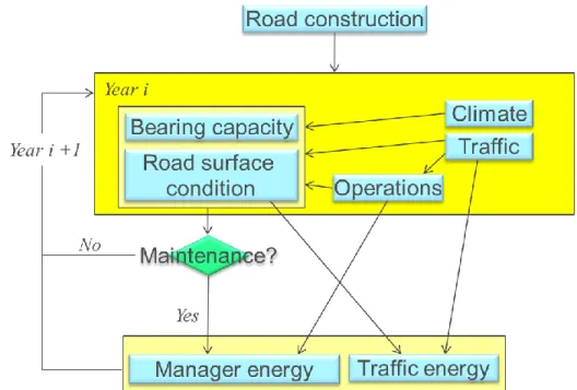
Calculation of total energy is a crucial part in order to draw conclusions on the influence of rolling resistance in energy use of road transport. Below is a simplified scheme for calculation that is used in the field studies. The overall principle is to map energy use over time, starting with construction, and predict future condition, maintenance needs and traffic energy during service life. Each step is detailed below, section by section.

(17)

Figure 1 Calculation of energy use in incremental steps. 2.3.1 Design of case studies

The two cases were selected based on the assumption that high volume traffic and poor evenness are two factors that can call for rolling resistance to become an aspect to consider when designing pavement maintenance. Generally, historical data on road surface

measurements regarding IRI and rut depth is accessible back to 1987 and for maintenance treatments the records are older. Mean profile depth (macro texture) was added to the common survey programme in 2006. It should be noted that the methods and equipment for road surface measurements have changed during time resulting in slight differences.

However, for the purpose of this study, these issues can be neglected. AADT is given per carriageway.

Both case studies are located in the south of Sweden.

Case 1 is one kilometer of road E20 in Örebro from Marieberg to E18 junction.

 2+2 lane motorway

 AADT year 2010 from TIKK1 database: o Total 19400 + 17400

o Trucks, no trailer 1001 + 887 o Trucks with trailer 1016 + 918

For Case 1 remixing (hot in-place) is proposed as main alternative. SMA11 and SMA8 are assessed as alternatives.

Case 2 is one kilometer on road 47 bypass Falköping.

 1+1 lane road over low, marshy land  Bypass built in 1992

 AADT year 2006 from TIKK database: o Total 4280

(18)

o Trucks, no trailer 275 o Trucks with trailer 458

For Case 2 main alternative proposed is local leveling treatments with patching and no overlay (continue as before). The alternative treatments are complete removal of bound layers, improved drainage and placement of unbound base layer and bound layers designed according to standard (significantly reduce IRI).

2.3.2 LCA Framework

Life cycle assessment (LCA) is a technique developed to assess and understand

environmental impacts of products, but processes and activities can also be studied. Since one of the purposes of LCA is to compare products, standardization of the assessment procedure is important to be able to compare assessment of different products. For this purpose a number of ISO standards have been created. Standardization becomes important also in pavement LCA. Pavements pose challenges to be defined as products since their design is very (highly) dependent on external conditions (traffic, climate, geology, topology, etc.). Introducing LCA to assess maintenance activities is also challenging. A principle for comparing alternatives in LCA is to express environmental impact per functional unit, i.e. the easiest approach is to study alternatives with equal functional performance. However, this is often not entirely possible. In the case of assessing maintenance alternatives with respect to road manager and traffic energy, evenness or texture need to be different in order to achieve the desired

differences between road manager and traffic energy. Therefore the system boundary in this case is expanded from the product (pavement) to also include the transport process (fuel use of vehicles). This means that the quality of service given by the transport sub-system studied must be fairly equal for an adequate analysis. Otherwise the assessment will be misleading for example if traffic chooses other routes or if service levels drop below acceptable levels. To reduce the complexity further, comparative studies is used here in which only differing components are accounted for. Furthermore, only inventory is performed and limited to energy for reasons discussed above.

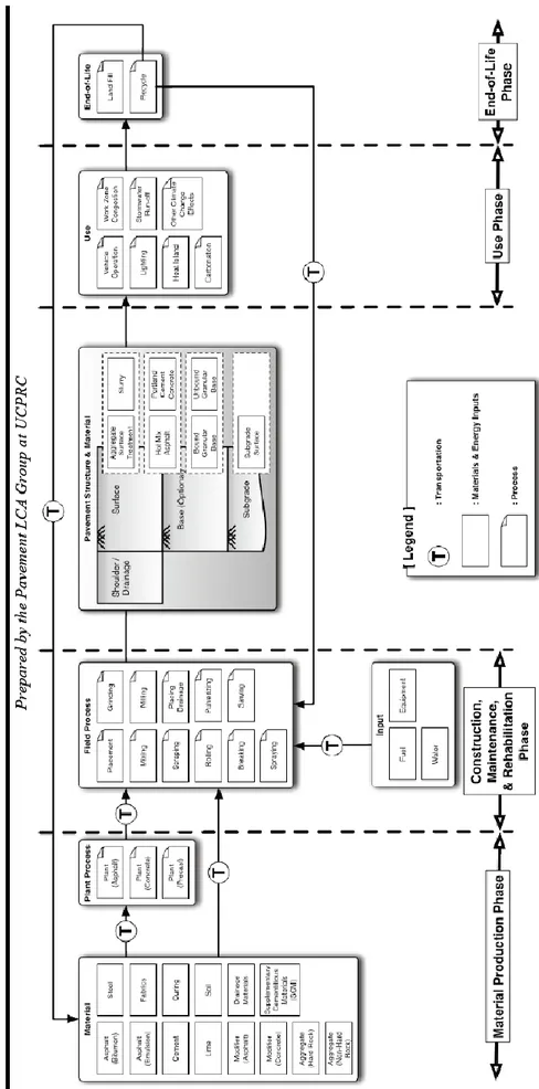
A workshop was organized by University of California at Davis (UC Davis, 2010), USA, in an effort to further shape a framework for LCA adopted for pavements and develop consensus on how to account for environmental impact of pavement management. The outcome is illustrated in the figure below and used as an overall principle in this report.

(19)

Figure 2 Framework proposed by UC Davis and discussed during workshop (UC Davis, 2010).

(20)

The framework illustrates the life cycle phases, including processes and material flows encountered in pavement systems. However, the workshop pointed out some areas that may need further attention:

 Accounting feedstock energy (bitumen)  Analysis period

 Functional unit for pavement LCA

 Approaches to object and network level LCA

 Material production accountancy such as net upgrading and view upon use of residuals (share burdens, i.e. oil refining)

 Downgrading of materials during recycling

The latter four issues will be addressed elsewhere in the report to aid in further development of practice. The former two issues are of great importance and further discussed here. Feedstock energy will not be included in the analysis. The reason is that the scope of this report aim towards the impact category “Global warming” and mixing bitumen with

aggregate will keep CO2 from being released from bitumen to atmosphere. This issue is part of a larger question on how to consider energy use in relation to the impact on environment. The authors believe that energy is a robust measure of environmental impact for some categories, among which Global warming is the focus of this report, as earlier discussed in Section 2.2.1.

The analysis period will be chosen based on the period maintenance measures can contribute to performance. If multiple measures are performed, or if the benefits of a measure will be significant beyond the next maintenance measure, a sufficiently long analysis period need to be chosen to include the complete benefit.

The calculations will be performed by inventory of all activities down to material flow levels or aggregated levels if no data is available. Calculation of energies will be based on a number of sources, further detailed in sections below.

2.3.3 Road construction energy calculations

In these cases, the study objects are existing roads and comparative studies are performed. This means that the road construction phase is excluded from the study. Only the pavement maintenance over a life cycle is considered. However, for the purpose of developing a general approach, it is of importance to acknowledge the road construction phase.

2.3.4 Road surface condition and bearing capacity

Road surface data has been collected from PMS and Väggrafen2 data. PMS include detailed data on 20 meter average for roughness (IRI), rutting and mean profile depth. Maximum values for rut depth and IRI are used (of left or right wheel path) and average macro texture (MPD) for left and right wheel path. Data back to 2006 was used. From Väggrafen data could be extracted back to 1987 for maximum rut depth and IRI reported as average over a section with homogeneous characteristics (road type, speed limit, etc.). This means that the section length can vary unlimited.

(21)

No data could be obtained on bearing capacity, but the evolution of IRI and information from pictures and maps was useful in identifying bearing capacity problems in case 2.

2.3.5 Climate

Since rolling resistance is influenced by the presence of snow or water on the road surface, it is of importance to know the proportions of these conditions. To find out how much water is left on the road surface, we need to know how much precipitation that actually falls on each test site. Then, this data is used to model drying sequences.

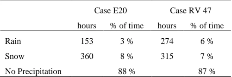
Climate data from one winter from representative nearby RWiS (Road Weather information System) outstations was chosen, in this case October 15 2004 to April 15 2005. This winter was chosen because the precipitation was close to normal (based on statistics 1961-1990). The number of hours with rain or snow fall can be seen in Table 1 for each outstation.

Table 1 Precipitation at the test sites, number of hours and percentage of time in the winter of 2004/05.

Case E20 Case RV 47

hours % of time hours % of time

Rain 153 3 % 274 6 %

Snow 360 8 % 315 7 %

No Precipitation 88 % 87 %

For the calculations of the amount of time the road surface is covered with water or moist, two sub-models of The VTI Winter Model3 used, “Splashing from a wet road” and “Drying of a moist road”. The first sub-model describes the variables that control the water disappearing from the road. Significant variables are traffic flow, the ratio between the number of cars and trucks, speed, wind speed and direction, road gradient and texture. This sub-model is used as long as the road is described as wet (>10 g/m2), and when the road turns to be moist the second sub-model take over. In this sub-model are calculations of the transition from moist to dry surface through evaporation done. The parameters taken into account are: road surface temperature, dew point temperature and wind speed, but also traffic flow, the ratio between the number of cars and trucks, speed, and salinity in the moisture.

2.3.6 Maintenance – treatment design and effects

The maintenance treatment design was based on the historical road surface conditions and the bearing capacity. From road surface condition data linear extrapolation of road surface

conditions was used by studying statistical parameters for evolution per year and variability in data year by year. This gave the likely year for intervention with respect to rutting, the share of section in need of longitudinal adjustments and the influence of bearing capacity

treatments. It was assumed that a bearing capacity treatment would lead to equal performance as during the first five years after the road was opened for traffic. To predict effects of various

3_{Winter is a model for winter maintenance strategies of roads and deals with the effects on accidents,}

accessibility (speeds and flows), fuel consumption, corrosion, environmental effects, the costs incurred by the road administration for the measures, and the costs of the road administration for wear.

(22)

sources of aggregate and maximum aggregate size, the VTI Wear model was used (Wågberg, Jacobson 1997).

2.3.7 Service life energy calculations

The next logical step is to assemble all the sub models described earlier to perform a life cycle analysis, as described in Figure 2. Traffic and maintenance energy calculations are complex to describe in detail and deserve a section on their own, cf. below.

The fuel use for cars and for trucks with and without trailer is estimated with the VETO model. A simulation is performed for each vehicle type and for each of the scenarios in the case studies. For a description of the scenarios see Sections 3.2 and 4.2. The vehicles used in the simulation represent average vehicles in Sweden. The alignment of the studied road sections is described fairly simplistic. Since the road sections in the case studies are straight and close to flat the gradient and horizontal radius are set to 0. The elevation is defined to 2.5 % which is the standard measurement for Swedish roads. The weather conditions is a standard weather with dry conditions, a wind speed of 2.5 m/s, air temperature is 8˚C and air pressure is 1.013 bar. Driving behavior is also described according to a standard driving behavior for Swedish roads and represents a state of free flow.

The road surface quality and road deterioration regarding IRI (roughness) and MPD (macro texture) is in the base scenario described according to the historical data that has been

gathered from PMS and Väggrafen. The road surface characteristics that results from different maintenance treatments are defined from Section 2.3.6.

The fuel use is estimated on a yearly basis and for a time period equal to the maintenance interval in each scenario. Fuel use is converted into energy and the total sum of energy use during the time period of the scenario is divided with the number of years in the time period. This will give an average yearly energy use that enables comparisons between the scenarios.

2.3.8 Analysis and implementation in decision making

The data collected in the case studies and the results from the manager and traffic energy calculations will be evaluated. The most important parameters regarding energy use will be sorted into a few tangible guidelines to aid in decision making.

2.4 VETO model

VETO is a simulation model in which the fuel consumption and exhaust emissions of vehicles can be estimated. It was originally developed to describe vehicle costs, including deterioration of tyres and brakes, repair cost and capital cost (Hammarström, Karlsson 1987). Lately, the model has primarily been used to estimate fuel consumption and exhaust emissions of traffic due to various characteristics of vehicles, roads and driving behaviour. It is a mechanistic model based on physical relationships in which it is possible to describe both vehicles and specific road segments with high precision.

VETO has been used to calculate traffic fuel use in the European projects IERD (2006), where it was integrated into the MX Software package, and in ECRPD (2010). It has also been used to estimate functions of fuel use and emission factors that have been integrated in

(23)

other models, for example EVA4, Winter-model5 and the EMV-model6. Furthermore VETO has been the tool for analysing various measures in the traffic environment (Nilsson et al 2005) and also to evaluate fuel use for different road alignments (IERD 2006).

The basic data in VETO can be divided into the following main parts:  Road

 Vehicle

 Driving behaviour  Weather

The road characteristics are the geometry, speed limit and surface. In this part the vertical and horizontal alignment is described, and also the length, width, super elevation and speed limits. The road section can be divided into segments and each segment can be defined with its own parameters. Road surface characteristics are set equal for the whole section and covers properties such as longitudinal roughness (IRI), macro texture (MPD), and the age of the surface course.

The vehicle data includes the type of vehicle, such as car, bus, truck or truck with trailer, air resistance, masses of empty vehicle, max load and load factor, and also axles and wheels. Engine is defined according to fuel type, swept volume and moment of inertia, engine power and auxiliaries use, idling, fuel cut off engine speed interval, max torque curve and engine fuel map. The characteristics of tyres are radius, width, rolling resistance, pressure, tyre tread and pattern, tyre slip and stiffness, and the type of vehicles it will be used for. The

transmission concerns the gear ratio and mechanical efficiency, and the rotating losses in the gear box.

In driving behaviour it is possible to define speed as a function of road width for various vehicles and it is also possible to combine this with a description of traffic situations such as free flow, heavy, saturated and “stop and go”. With gear change one can define the use of max torque during acceleration and for steady state speed, deceleration and gear change decisions. Data for weather conditions comprise of wind speed and special wind angles, air temperature and air pressure, snow depth and density, and water depth.

The various input parameters can be changed to investigate vehicles energy under different conditions.

In the MIRIAM project VETO is used to evaluate fuel use of traffic due to different values of roughness and macro texture. The vehicles and driving behaviour represent typical Swedish conditions. The roads in the case studies, E20 and RV47, are fairly flat and straight, and both geometrical and vertical alignment is set to 0. The super elevation is 2.5 % and the widths of the roads are 13 m for E20 and 9 m for RV47. Speed limit is 110 km/h for E20 and 90 km/h for RV47. The weather is a standard weather and dry conditions with 8˚C, a wind speed of 2.5 m/s. In the simulations these parameters are unchanged. Only the IRI and MPD are varied according to the different maintenance alternatives and the estimated road surface

deterioration as described in 3.2 and 4.2.

4

The EVA model is a tool that is used in the planning process of an individual road or a traffic system and it estimates effects and public economy.

5_{Winter is a model for winter maintenance strategies of roads and deals with the effects on accidents,}

accessibility (speeds and flows), fuel consumption, corrosion, environmental effects, the costs incurred by the road administration for the measures, and the costs of the road administration for wear.

(24)

The fuel use in dm3/10 km is estimated for one type of vehicle according to the defined parameters in the model. To calculate the expected fuel use for one year, the figure in dm3/10 km for each vehicle type is transformed to MJ/ (km road section) and multiplied with the AADT for the specific vehicle type. The energy use for the different vehicle types are added together to get the total yearly traffic energy use for the road section in the case study. This procedure makes it easy to study the effect of fuel use due to various developments of the traffic flow and also due to different structures of the traffic and characteristics of the road. For free flow on road link the following model for fuel consumption (Fcs) of cars was derived (similar models existing for heavy trucks and heavy trucks with trailers) in a parallel

MIRIAM sub project, assuming typical car data, conditions and driving patterns using models implemented in VETO (Hammarström et al, 2012):

Fcs=0.286*((1.209+0.000481*IRI*v+0.0394*MPD+0.000667*v^2+0.0000807*ADC*v^2 -0.00611*RF+0.000297*RF^2)^1.163)*v^0.056 [liter per 10 km]

where

v = vehicle speed [m/s]

ADC = road curvature [rad per km] RF = slope [m per km]

It should be noted that the above relationship is nonlinear and cannot easily be simplified to break out the contributions of MPD and IRI to fuel consumption.

2.5 Pavement maintenance energy calculations

The energy calculations for maintenance are based on treatment designs. Traditional designs are considered while the authors are aware of recent year’s interest and development of low energy solutions for maintenance. The purpose of selecting traditional designs as a norm is to establish a baseline and promote the use of low energy solutions in relation to this baseline. Below is summary of the primary and secondary energy figures derived later in this section, which are used in the calculations of maintenance energies.

Primary Secondary

Bitumen 3.7 3.36 MJ/kg

Aggregate 50 40 MJ/ton

Transport 1.54 1.40 MJ/ton*km (one way)

Asphalt plant 280 230 MJ/ton

Placing 3.0 2.73 MJ/m2

(25)

2.5.1 Bitumen production and supply

Bitumen energy calculations include a number of issues that need attention. Here, the total energy related to bitumen at the point of deliver to asphalt plant is described. The steps involved are:

 Heavy crude oil extraction  Transport

 Refining (atmospheric distillation, vacuum distillation, solvent fractionation, blowing)  Transport and storage at depots

 Transport to asphalt plants

Three major issues are feedstock (intrinsic) energy and other products manufactured during the process and the fact that bitumen is extracted, refined and used at different locations using different means and methods. As motivated elsewhere, feedstock energy will be separately accounted for. Manufacture of other products pose a problem since it is difficult to objectively allocate the common share of energy used to each product. Examples of other products

manufactured during along with bitumen are lubricants, transformer oils, hydraulic oils and process oils. According to ISO 14044, allocations shall be done in the following order: (1) mass units, (2) economic units, (3) the number of times the product can be recycled. In the LCI presented by Eurobitume (Eurobitume, 2011), mass allocation is used for extraction and transport and economic allocation is used in the subsequent refining steps.

The cost allocation for refining by Eurobitume arrives at 27 % share for bitumen. Stripple assumed 40 % in his study (Stripple, 1995). According to Eurobitume there is great variation in energy use during crude oil extraction between different countries. Stripple use Swedish conditions with Venezuelan crudes. According to Eurobitume, crude oil extraction in South America uses substantially more energy than in Former Soviet Union countries, which dominate the European market.

In this report an energy use of 3.70 MJ/kg (secondary 3.36 MJ/kg) for bitumen according to Stripple is used, bearing in mind that this is relevant to Swedish conditions but may be difficult to directly compare to European conditions. According to the inventory made by Eurobitume, the energy use calculated based upon their inventory data seems comparable, even though the energy generated from uranium is difficult to compare.

2.5.2 Aggregate production and supply

Studies by Stripple (1995), Linden (2008) and (Andersson and Gunnarsson, 2009) give roughly the same total energy use for production, even though the source proportion of electricity and diesel varies. The data reported by Andersson and Gunnarsson give secondary energies of 30 and 45 MJ/ton crushed aggregate for two and three crushings, respectively. Three crushings are needed for production of aggregate to wearing courses. Stripple report 38 MJ/ton aggregate but does not specify the number of crushings.

Here 50 MJ/ton of primary energy is used. The corresponding secondary energy is estimated to 40 MJ/ton.

2.5.3 Asphalt concrete mix design and production

Stripple report use of 80 MJ/ton of electricity and 285 MJ/ton of heating oil (Stripple, 1995), corresponding to secondary energies of 36 MJ/ton electricity and 259 MJ/ton heating oil.

(26)

This is somewhat higher than reported by Lindén: 9 and 227 MJ/ton of secondary energy, respectively. An LCA study within the ECRPD project report values similar to Stripple for heating, while the reported electricity use is half.

It is believed that recent year’s efforts to lower energy use have led to more efficient plants with less energy losses. However, the heat energy input for hot asphalt concrete is in the order of 140 MJ/ton based on a heat capacity of 900 J/kgK. Here, a total of 280 MJ/ton is used (secondary 230 MJ/ton).

2.5.4 Transport

Transport of materials related to asphalt concrete can be divided into:

 Oil from source to refinery and bitumen from refinery to storages (included in section on bitumen production and supply)

 Aggregate from quarry to asphalt plant  Asphalt concrete to site

High performance wearing course materials are often transported long distances since the properties are of utmost importance to the properties of the resulting road surface regarding for example skid resistance, wear resistance and light reflection. In line with the scope of this report, conflicts can be identified in that low rolling resistance materials may need superior materials, which may require longer transport. The transport distance is of course dependent on the distance to available quarries and the possibilities to transport material by train or ship. Hence, the energy used for transport of wearing course material is very site and solution specific. Sweden has generally good rock and no train or ship transport is needed in the cases. Here the need for energy is based on that a fully loaded truck use 0.50 liter diesel per km and takes 33 tons. On return it use 0.26 liter diesel per km. With a primary energy of 38.61 MJ/liter diesel the energy use become 1.54 MJ per ton aggregate and kilometer distance between quarry and plant. The corresponding secondary energy become 1.4 MJ/ton.

2.5.5 Equipment

ECRPD uses 6.5 MJ/m road for asphalt concrete laying, 4.0 MJ/m road for compaction, 16 MJ/m road for milling. Furthermore, ECRPD give a value of 137 MJ/m road for remixing. Assuming two 4 meter lane width give the following figures [MJ/m2]: laying 0.8, compaction 0.5 and milling 2.0. Remixing become 20 MJ/m2 if two 3.5 m widths are treated. This has to be considered as an underestimation since we know that about 50 MJ/m2 is used in heating with IR gas heaters.

Stripple data show around 0.7 MJ/ m2 for asphalt concrete laying, 0,6 MJ/ m2 for compaction, and 1.7 MJ/m2 for milling.

In this report 3.0 MJ/m2 (secondary 2.7 MJ/m2) is used for placing conventional asphalt concrete and 58.3 MJ/m2 (secondary 53 MJ/m2) for remixing.

(27)

3 Case study E20 Örebro

3.1 Road surface measurements and data

3.1.1 Climate

Results from calculations of distribution of dry, moist and wet road surface based on the Winter model and the weather conditions of the location are presented in Table 2.

Table 2 Distribution of road surface condition. Number of hours and percentage of time in the winter of 2004/05. Case E20 hours % of time Dry road 3144 72 % Moist road <10 g/m2 463 11 % Wet road >10 g/m2 784 18 % 3.1.2 Condition history

Below is the historical mean rut depth for homogenous sections of various lengths from 1987 to 2008 with slightly different limits compared to the sections studied (33446-34446), and the average rut depth calculated from PMS data for the sections studied. Typical “shark-teeth” patterns appear. On the average 3.4 mm of rut is developing per year when no treatment is performed.

Figure 3 Rutting per section [mm].

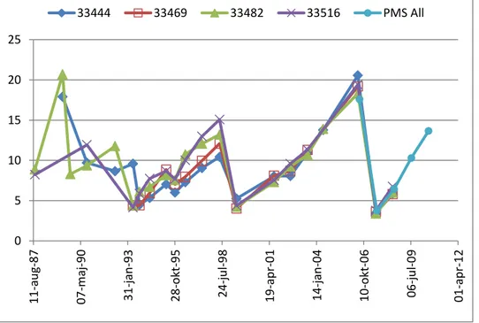
There is a small increase in IRI indicated in the figure below from 2007 to 2010, but this difference is not significant when looking at the actual data. Therefore it can be assumed that IRI will not change significantly as a result of decisions on when and how to maintain this particular road. 0 5 10 15 20 25 11 -au g-8 7 07 -m aj -90 31 -ja n -93 28 -o kt -9 5 24 -ju l-9 8 19 -ap r-0 1 14 -ja n -04 10 -o kt -0 6 06 -ju l-0 9 01 -ap r-1 2 33444 33469 33482 33516 PMS All

(28)

Figure 4 IRI per section [mm/m].

Figure 5 Average macro texture in the right (MPDH) and left (MPDV) lane with 20 and 80 percentile [mm].

3.1.3 Spatial variation in condition

In order to identify the deterioration mechanisms and the expected development of

performance indicators, individual sections where analyzed. When comparing data from 2006 with data from 2010 it becomes evident that the development in road condition can be

classified in sections with better and worse development. This indicates that treatments addressing local problems could be beneficial. However, the difference between the sections is not alarming and acceptable conditions can be reached with all treatment strategies

suggested below. 0 0,5 1 1,5 2 2,5 3 11 -au g-8 7 07 -m aj -90 31 -ja n -93 28 -o kt -9 5 24 -ju l-9 8 19 -ap r-0 1 14 -ja n -04 10 -o kt -0 6 06 -ju l-0 9 01 -ap r-1 2 33444 33469 33482 33516 "PMS All" 0 0,2 0,4 0,6 0,8 1 1,2 1,4 2005-05-28 2006-10-10 2008-02-22 2009-07-06 2010-11-18 MPDH MPDV

(29)

Figure 6 Rutting per section and year [mm].

Figure 7 IRI per section and year [mm/m].

3.2 Maintenance strategies and their influence on road condition

Rutting is the criteria triggering decision on when to perform maintenance. This means that any maintenance strategy to lower rolling resistance has to meet the requirements related to resistance to rutting.

Three scenarios for maintenance was selected and compared to a fourth scenario of doing no maintenance. The fourth scenario is interesting to illustrate the hypothetical importance of rutting for rolling resistance, especially during wet or snowy conditions. The three main scenarios for maintenance are:

1. Remixing. The option chosen by the pavement management. Deliver very good evenness but slightly higher rate of rutting compared to other alternatives. 20 % new material is needed to account for the ruts and 80 % is recycled asphalt concrete 0,0 5,0 10,0 15,0 20,0 25,0 33200 33400 33600 33800 34000 34200 34400 34600 2006 2007 2008 2009 2010 0,0 0,5 1,0 1,5 2,0 2,5 33200 33400 33600 33800 34000 34200 34400 34600 2006 2007 2008 2009 2010

(30)

2. The very low IRI and low MPD alternative. Milling and placing a binder layer and a wearing course of SMA11 with state of the practice equipment to achieve evenness. 3. The very low MPD alternative. SMA8 with very small maximum aggregate size is

used. To ensure wear resistance and durability, high performance aggregate and slightly higher binder content are chosen. In practice some more modification might be needed such as modifiers and more controlled aggregate grading.

The period chosen for analysis of when to do maintenance was summer 2011, since this was the time planned for doing remixing on this particular road section.

Table 3 Description of maintenance scenarios and expected future condition

Scenario: 0 1 2 3

Length treated: [%] 0 % 100 % 100 % 100 %

Date of treatment: 2011-07-15 2011-07-15 2011-07-15

Type of treatment na Remixing SMA11/ ABS11

Binder layer

SMA8/ ABS8

Asphalt concrete, mean [mm] 0 40 33+40 30

Rut after treatment: [mm] 17 3 2 3

IRI after treatment: [mm/m] 0.9 0.7 0.7 0.8

Slope Rut: [mm/y] 3.4 3.4 2.0 3.5

Slope IRI [mm/m·y] 0.04 0.04 0.02 0.04

Below is the resulting rut depth and IRI based on the above assumptions regarding treatments. Levels of acceptance are indicated in red: 13 mm for ruts and 2.6 mm/m for IRI. These levels should only be seen as indicative levels and not as requirements.

Figure 8 Rutting predicted for the scenarios [mm]. 0 5 10 15 20 25 1995-10-28 2001-04-19 2006-10-10 2012-04-01 2017-09-22 2023-03-15

(31)

Figure 9 IRI predicted for the scenarios [mm/m].

With respect to the standard levels indicated in Figure 8 above one can conclude that maintenance was needed already in 2010, a year before maintenance was actually done (2011).

The following MPD values are assumed for the four scenarios: 0. 0.75 mm

1. 0.75 mm year 2 and onwards, 1.00 year 1 2. 0.70 mm year 2 and onwards, 0.95 year 1 3. 0.60 mm year 2 and onwards, 0.8 year 1

3.3 Manager energy calculations

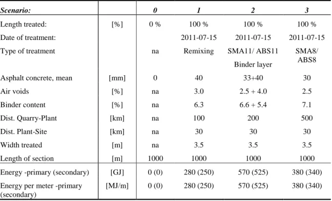
Based on technical specifications, experience of maintenance scenarios and case specific conditions, the resource needs for different maintenance alternatives were calculated. The results are presented in the table below.

0 1 2 3 4 5 1995-10-28 2001-04-19 2006-10-10 2012-04-01 2017-09-22 2023-03-15

(32)

Table 4: Assumptions for calculations of energy related to maintenance treatments and resulting primary and secondary energies.

Scenario: 0 1 2 3

Length treated: [%] 0 % 100 % 100 % 100 %

Type of treatment na Remixing SMA11/ ABS11

Binder layer

SMA8/ ABS8

Asphalt concrete, mean [mm] 0 40 33+40 30

Air voids [%] na 3.0 2.5 + 4.0 2.5 Binder content [%] na 6.3 6.6 + 5.4 7.1 Dist. Quarry-Plant [km] na 100 200 500 Dist. Plant-Site [km] na 30 30 30 Width treated [m] na 3.5 3.5 3.5 Length of section [m] 1000 1000 1000 1000

Energy -primary (secondary) [GJ] 0 (0) 280 (250) 570 (525) 380 (340) Energy per meter -primary

(secondary)

[MJ/m] 0 (0) 280 (250) 570 (525) 380 (340)

3.4 Traffic energy calculations

The traffic fuel use on E20 is estimated for Scenario 1, 2 and 3 using the VETO model described in Section 2.4. The option of doing nothing is not an alternative since rutting has reached the level of what is recommended, see Figure 8. Input data for roughness and macro texture is according to the description in 4.2. The number of years for each scenario is decided by the requirements of road conditions as described in Figure 8 and Figure 9 and it is rutting that is the limiting factor in all of the scenarios for E20. In Scenario 1, where the whole road section is treated with remixing, it takes approximately four years before a new treatment is needed. This is also the case in Scenario 3 where SMA8/ABS8 is used. Using SMA11/ABS11 as material, Scenario 2, implies that it would take six years before there is a need for a new intervention.

Figure 10 presents the yearly total secondary energy use of traffic on E20 and in the north-bound lanes. For the treatment alternatives Remixing and SMA8/ABS8 the time period is set to six year, which is equal to the alternative SMA11/ABS11, with an assumption that no further treatment is performed than the initial one. Also the estimations for year 5 and 6 are only displayed to show the development of traffic energy use and they are bars not included in the average yearly energy use for Scenario 1 and Scenario 3. Therefore, the bars are slightly transparent in the figure. If treatment would be performed, it is expected that the energy use of traffic would follow the same development as year 1 to year 4. Cars constitute 90 % of the traffic and have a 65 % share of the total energy use. Trucks and trucks with trailer have each a 5 % share of traffic but are responsible for 35 % of energy use.

As can be seen in the figure, there is no substantial difference in the resulting traffic energy use between the different treatment methods. In all scenarios, the energy use in year 2 is less compared to year 1, which depends on the reduction of macro texture (MPD). This reduction is assumed to only happen in year 2 and MPD are thereafter constant in the simulation. Thereby, all differences in energy use after year 2 are because of changes in roughness (IRI).

(33)

Remixing leads to the highest average traffic secondary energy use per year, 20,169 GJ/year. For SMA11/ABS11 and SMA8/ABS8 it amounts to 20,112 and 20,075 GJ/year respectively. However, the differences in total energy use are small between the alternatives, at the most 94 GJ for one average year, a difference of 0.5 %. This depends mainly on the high overall standard of the road and the different treatment alternatives leads to relative minor

improvements in MPD and IRI. Also, the high share of cars may be a part of the explanation since their fuel use are relative small in comparison with trucks and trucks with trailers and thereby is the fuel use not as sensitive to changes in road surface characteristics as it would be if trucks had a larger share.

The average primary energy use for the same treatments are 22,186 GJ/year for Remixing, 22,123 GJ/year for SMA11/ABS11 and 22,083 GJ/year for SMA8/ABS8.

Figure 10 Secondary energy use traffic, E20 northbound lanes.

3.5 Total energy calculations, GJ/year

Service Manager energy Traffic energy Total energy

Treatment life Secondary Primary Secondary Primary Secondary Primary

Remixing 5 50 56 20,169 22,108 20,219 22,164 SMA11/ ABS11 6 87.5 95 20,112 22,123 20,200 22,218 SMA8/ ABS8 5 68 76 20,075 22,083 20,143 22,159 20 000 20 050 20 100 20 150 20 200 20 250 20 300 1 2 3 4 5 6 GJ/y e ar Year Remixing SMA11/ABS11 SMA8/ABS8

Average secondary energy use:

Remixing 20 169 GJ/year SMA11/ABS11 20 112 GJ/year SMA8/ABS8 20 075 GJ/year

(34)

4 Case study Road 47 Falköping

4.1 Road surface measurements and data

4.1.1 Climate

Table 5 Distribution of dry, moist and wet road surface conditions. Number of hours and percentage of time in the winter of 2004/05.

Case Rv 47 hours % of time Dry road 2356 54 % Moist road <10 g/m2 643 15 % Wet road >10 g/m2 1392 32 % 4.1.2 Condition history

Below is the historical mean rut depth and the corresponding 90 percentile. On the average 1.3 mm of rut is developing per year when no treatment is performed. The data presented is average for the whole length.

Figure 11 Rutting. Average and 90-percentile for the whole length per year [mm]. 0 5 10 15 20 25 1-Ap r-9 3 1-Ma r-9 4 1-Fe b -95 1-Jan -96 1-De c-96 1-N o v-97 1- Oct-98 1-Se p -99 1-Au g-0 0 1-Ju l-01 1-Ju n -0 2 1-Ma y-03 1- Apr-0 4 1-Ma r-0 5 1-Fe b -06 1-Jan -07 1-De c-07 1-N o v-08 1- Oct-09 1-Se p -10 Rut_mean Rut_P90

(35)

Figure 12 IRI. Average and 90-percentile for the whole length per year [mm/m]. 4.1.3 Spatial variation in condition

In order to identify the deterioration mechanisms and the expected development of

performance indicators, individual sections where analyzed. However, for various reasons, the trends appeared more or less stochastic, especially with respect to IRI, cf. Figure 14. Some sections have very high rut depth development, up to 3.5 mm per year 2008-2010. No modeling of rut depth development on individual sections were possible but the section data could be used to estimate the resulting condition after maintenance based on which sections that was selected for treatment.

Figure 13 Rutting per 20 meter section 2006-2010 [mm]. 0 1 2 3 4 5 1-Ap r-9 3 1-Fe b -94 1-De c-94 1- Oct-95 1-Au g-9 6 1-Ju n -9 7 1-Ap r-9 8 1-Fe b -99 1-De c-99 1- Oct-00 1-Au g-0 1 1-Ju n -0 2 1-Ap r-0 3 1-Fe b -04 1-De c-04 1- Oct-05 1- Aug-0 6 1-Ju n -0 7 1-Ap r-0 8 1-Fe b -09 1-De c-09 1- Oct-10 IRI_mean IRI_P90 0 5 10 15 20 25 30 35 21500 22000 22500 23000 23500 24000 24500 2006 2008 2009 2010 Slope

(36)

Figure 14 IRI per section 2006-2010 [mm/m].

4.2 Maintenance strategies and their influence on road condition

Based on the road condition the worst sections were selected for treatment with three scenarios: 15 % of the length, 30 % of the length and the total length (100 %). This was compared to if no treatment would be applied (0 %). By looking at the slope of existing data and experience of data collected from other roads the conditions for future road conditions were calculated for the four scenarios. The period chosen for analysis of when to do

maintenance was subject to discussions but in the end an historic date of mid July 2007 was chosen. There was enough data before 2007 and it was considered to be an advantage to have data after the treatment date for comparison. The authors do not have the knowledge of the exact type and extent of the treatments made in 2007 but the treatment seems to have covered about 30-40 % of the length.

Table 6 Description of maintenance scenarios and expected future condition

Scenario: 0 1 2 3

Length treated: [%] 0 % 100 % 15 % 30 %

Type of treatment na drainage,

milling, levelling, new AC milling, levelling, new AC milling, levelling, new AC

Asphalt concrete, mean [mm] 0 100 50 50

Rut after July 2007: [mm] 17 3 15 12

IRI after July 2007: [mm/m] 3.52 1.0 3.1 2.6

Slope Rut after treatment: [mm/y] - 1.0 1.3 1.3

Slope IRI after treatment: [mm/m·y] - 0.15 0.20 0.20

Slope Rut if no treatment [mm/y] 3.5 - 2.0 2.0

Slope IRI if no treatment [mm/m·y] 0.30 - 0.25 0.25

Scenario 1 considers a more thorough treatment with a more complete milling and buildup of road surface to enhance evenness. This should result in conditions similar to new standard.

0 1 2 3 4 5 6 7 21500 22000 22500 23000 23500 24000 24500 2006 2008 2009 2010

(37)

The assumptions regarding increase in rut depth and IRI for scenario 1 is based on the

conditions five years after opening the road for traffic in (1993) and for the other scenarios the measurements from 2003 and onwards, thus considering the difference between the present structural standard and the structural standard that could be expected after rehabilitation. Below is the resulting rut depth and IRI based on the above assumptions regarding treatments. Levels of acceptance are indicated in red: 14 mm for ruts and 3.2 mm/m for IRI. These levels should only be seen as indicative levels and not as requirements.

Figure 15 Rutting predicted for the scenarios [mm].

Figure 16 IRI predicted for the scenarios [mm/m].

With respect to the standard levels indicated in the figures above one can conclude that maintenance was needed already in 2006. Furthermore, maintenance covering 15 % of the length, removing the sections in worst condition would not have met the requirements after

0 5 10 15 20 25

28-okt-95 19-apr-01 10-okt-06 01-apr-12 22-sep-17 15-mar-23

Rut_mean 0% 100% 15% 30% 0,0 0,5 1,0 1,5 2,0 2,5 3,0 3,5 4,0 4,5 5,0

28-okt-95 19-apr-01 10-okt-06 01-apr-12 22-sep-17 15-mar-23

(38)

one year. Still, it is of interest to keep the 15 % scenario (2) to be able to assess if the standard levels can be defended from an energy point of view.

For all these cases MPD can be assumed to be 1.00 mm during the year after treatment and 0.75 mm during the following years. This means MPD for the different scenarios:

0. 0.75 mm all years

1. 1.00 mm year 1, 0.75 mm following years 2. 0.79 mm year 1, 0.75 mm following years 3. 0.83 mm year 1, 0.75 mm following years

4.3 Manager energy calculations

Based on technical specifications, experience of maintenance scenarios and case specific conditions, the resource needs for different maintenance alternatives were calculated. The results are presented in the table below.

Table 7 Assumptions for calculations of energy related to maintenance treatments and resulting primary and secondary energies.

Scenario: 0 1 2 3

Length treated: [%] 0 % 100 % 15 % 30 %

Type of treatment na drainage,

milling, levelling, new AC milling, levelling, new AC milling, levelling, new AC

Asphalt concrete, mean [mm] 0 100 50 50

Air voids [%] na 2.7 2.7 2.7

Binder content [%] na 6.4 6.4 6.4

Dist. Quarry-Plant [m] na 100 100 100

Dist. Plant-Site [m] na 50 50 50

Width treated [m] na 4 4 4

Total length of section [m] 2096 2096 2096 2096

Energy [GJ] 0 1700 (1490) 130 (110) 260 (230)

Energy per meter: [MJ/m] 0 810 (710) 62 (54) 124 (108)

4.4 Traffic energy calculations

The fuel use of traffic on Rv 47 is estimated for Scenario 1, 2 and 3. This is done even though only scenario 1 and 3 will meet the requirement of satisfying road conditions regarding ruts and roughness. Scenario 2 is included to demonstrate the development of fuel use if these requirements would allow for a lower road standard. The alternative of doing nothing is not a viable option and is therefore not studied. The input data for roughness and macro texture is according to the description in 4.2. The number of years for each scenario is mainly decided by the requirements of road conditions as described in Figure 15 and Figure 16. In Scenario 1, where the whole road section is treated with drainage, milling, leveling and new AC, it takes sixteen years before roughness reaches the recommended level. The time span for rut is shorter and the level is reached after twelve year, why this is the number of years the fuel use