Vehicle lateral position depending on road type and lane width : vehicle position surveys carried out on the Swedish road network

(1)

Terence McGarvey

Vehicle lateral position depending on

road type and lane width

Vehicle position surveys carried out

on the Swedish road network

VTI r apport 892A | V ehicle later al position depending on r www.vti.se/en/publications

VTI rapport 892A

Published 2016

(2)

(3)

VTI rapport 892A

Vehicle lateral position depending on road

type and lane width

Vehicle position surveys carried out

on the Swedish road network

(4)

Reg. No., VTI: TRV2012/53335 Cover pictures: Terence McGarvey

(5)

Abstract

In previous studies it was found that vehicle lane position varied depending on road type and lane width. These variations will have a direct effect on the rate of surface wear and will influence where stresses and strains are distributed in the pavement structure.

In order to quantify these variations, a series of position surveys were carried out on common road types found on the Swedish road network. Twenty-one sets of data provided information on over 271,000 vehicles.

It was possible to split vehicles into three categories and calculate average positions and standard deviations. Values were then used to describe the distribution of lateral position (wheel path), average position, and variation of lateral position (lateral wander).

Factors such as lane type, lane width, verge width, total width, and close proximity of guardrail all had some influence on vehicle position and amount of lateral wander. The extent of lateral wander varied quite considerably. Values associated with light vehicles varied between 455 millimetres and

190 millimetres. Commercial traffic values were lower and ranged between 430 millimetres and 140 millimetres.

These large variations will have a significant effect on road degradation rates and should be taken into account when planning construction or maintenance work.

Title: Vehicle lateral position depending on road type and lane width.

Vehicle position surveys carried out on the Swedish road network.

Author: Terence McGarvey (VTI, www.orcid.org/0000-0002-6198-0888)

Publisher: Swedish National Road and Transport Research Institute (VTI)

www.vti.se

Publication No.: VTI rapport 892A

Published: 2016

Reg. No., VTI: TRV2012/53335

ISSN: 0347-6030

Project: Vehicle lateral position depending on road type and lane width

Commissioned by: Swedish Transport Administration

Keywords: Vehicle Position, Road Type, Lane Width, Lateral Wander, Wheel

Path, Surface Wear, Deformation

Language: English

(6)

Referat

I tidigare studier om mötesfria vägar har det rapporterats att ett fordons sidolägesfördelning varierar beroende på vägtyp och filbredd. Variationer i ett fordons sidoläge har en direkt effekt på vägyte-slitage och påverkar hur spänningar och töjningar fördelas i överbyggnadsstrukturen.

För att fastställa omfattningen av dessa variationer har en rad undersökningar på sidolägen utförts på vanligt förekommande vägtyper i det svenska vägnätet. Information om mer än 271 000 fordon utvanns ur tjugoen datauppsättningar.

Undersökningsdatan gjorde det möjligt att dela upp fordon i tre grupper, beräkna sidoläge medelvärde och standardavvikelse samt sammanfatta sidolägesfördelning, genomsnittligt sidoläge och sidoläges-variation.

Faktorer som körfältstyp, körfältsbredd, vägrensbredd, total bredd och avstånd till skyddsräcke påverkade alla sidoläge och sidoförflyttning. Omfattningen av sidoförflyttning varierade väsentligt. Värden för lätta motorfordon varierade mellan 190 millimeter och 455 millimeter. Värdena för tung trafik var lägre och varierade mellan 140 millimeter och 430 millimeter.

Detta är stora variationer som kommer att ha en betydande effekt på vägars nedbrytningstakt. De bör därför tas med i beräkningen vid planering av konstruktions- eller underhållsarbete.

Titel: Fordons variation i sidled beroende på vägtyp och körfältsbredd.

Undersökningar på fordons sidolägen utförts på det svenska vägnätet

Författare: Terence McGarvey (VTI, www.orcid.org/0000-0002-6198-0888)

Utgivare: VTI, Statens väg och transportforskningsinstitut

www.vti.se

Serie och nr: VTI rapport 892A

Utgivningsår: 2016

VTI:s diarienr: TRV2012/53335

ISSN: 0347-6030

Projektnamn: Fordons variation i sidled beroende på vägtyp och körfältsbredd

Uppdragsgivare: Trafikverket

Nyckelord: Fordons Sidoläge, Väg Typ, Körfältsbredd, Sidolägesvariation.

Sidolägesfördelning, Vägyteslitage, Nedbrytning

Språk: Engelska

(7)

Foreword

This project was funded by the Swedish Transport Administration (Trafikverket).

Investigations, data analysis, and report writing have been carried out by Terence McGarvey (VTI). Thanks are extended to Håkan Wilhelmsson (VTI) and Sven-Åke Lindén (formerly of VTI) who carried out the vehicle position surveys and to Olle Eriksson (VTI) for his assistance with the interpretation of the measurement data.

Linköping, June 2016

Terence McGarvey Project leader

(8)

Quality review

Internal peer review was performed on 10 February 2016 by Leif Sjögren. Terence McGarvey has made alterations to the final manuscript of the report. The research director Anita Ihs examined and approved the report for publication on 30 May 2016. The conclusions and recommendations expressed are the author’s/authors’ and do not necessarily reflect VTI’s opinion as an authority.

Kvalitetsgranskning

Intern peer review har genomförts 10 februari 2016 av Leif Sjögren. Terence McGarvey har genomfört justeringar av slutligt rapportmanus. Forskningschef Anita Ihs har därefter granskat och godkänt publikationen för publicering 30 maj 2016. De slutsatser och rekommendationer som uttrycks är författarens/författarnas egna och speglar inte nödvändigtvis myndigheten VTI:s uppfattning.

(9)

Summary

Vehicle lateral position depending on road type and lane width. Vehicle position surveys carried out on the Swedish road network

by Terence McGarvey (VTI)

In previous studies of barrier separated road types, it was found that vehicle lane position and the amount of lateral wander varied depending on road type and lane width.

Variations in vehicle lane positon and the amount of lateral wander will have a direct effect on the rate of surface wear and will influence where stresses and strains are distributed in the pavement structure. In order to determine the extent of these variations, a series of position surveys were carried out on common road types found on the Swedish road network:

 conventional (7.7 m wide to 9.4 m wide),  motorway,

 barrier separated (2+1),  barrier separated (1+1),  four lanes, and

 conventional (13 m with wide side verge).

Twenty-one sets of survey data provided information on over 271,000 vehicles. The data was divided into three groups depending on approximate axle track width:

 light vehicles (1.5 m track width),

 heavy goods vehicle 1 (1.8 m track width), and  heavy goods vehicle 2 (2.1 m track width).

Using the survey data, it was possible to calculate and plot the distribution of lateral position (also called wheel path), the average position, and the variation of lateral position (also called lateral wander) for each group.

Factors such as lane type, lane width, verge width, total width, and close proximity of guardrail all had some influence on vehicle position and amount of lateral wander.

The extent of lateral wander varied quite considerably. Values associated with light vehicles varied between 455 millimetres and 190 millimetres. Commercial traffic values were lower and ranged between 430 millimetres and 140 millimetres.

These are large variations and will have a significant effect on road degradation rates. Such variations should be taken into account when planning construction or maintenance work.

(12)

(13)

Sammanfattning

Fordons variation i sidled beroende på vägtyp och körfältsbredd

av Terence McGarvey (VTI)

I tidigare studier om mötesfria vägar har det rapporterats att ett fordons sidoläge varierar beroende på vägtyp och körfältsbredd.

Variationer i ett fordons sidoläge har en direkt effekt på vägyteslitaget och påverkar hur spänningar och töjningar distribueras i överbyggnadsstrukturen.

För att fastställa omfattningen av dessa variationer har en rad sidolägesmätningar utförts på vanligt förekommande vägtyper i det svenska vägnätet:

 Traditionell väg (7,7 – 9,4 m bred)  motorväg

 mötesfri väg (2+1)  mötesfri väg (1+1)  fyrfilig väg

 traditionell väg (13 m med bred vägren).

Information om mer än 271 000 fordon utvanns ur tjugoen datauppsättningar. Data delades in i tre grupper beroende på axelspårvidd:

 Lätta motorfordon (1,5 m spårvidd)  tunga lastfordon 1 (1,8 m spårvidd)  tunga lastfordon 2 (2,1 m spårvidd).

Insamlad data gjorde det möjligt att beräkna och kartlägga sidolägesfördelning, genomsnittligt sidoläge och variation i sidoläge för varje grupp.

Faktorer som körfältstyp, körfältsbredd, vägrensbredd, total bredd och avstånd till skyddsräcke påverkade alla sidoläge och sidoförflyttning.

Det var stora skillnader i sidolägesvariationen beroende på fordons- och vägtyp. Värden för lätta motorfordon varierade mellan 190 millimeter och 455 millimeter. Värdena för tung trafik var lägre och varierade mellan 140 millimeter och 430 millimeter.

Detta är stora variationer som kommer att ha en betydande effekt på vägars nedbrytningstakt. De bör därför tas med i beräkningen vid planering av konstruktions- eller underhållsarbete.

(14)

(15)

1. Introduction

This report summarises a research project carried out on behalf of the Swedish Road Administration (Trafikverket).

In a recently finished but not yet published VTI Project (McGarvey, 2016), studies have revealed that vehicle position and confinement levels can vary depending on road type and lane width. For example, comparisons between conventional road types and barrier separated road types indicated that in the single lane section of a “2+1” barrier separated road, vehicle lateral wander reduced by 24% for light vehicles and 19% for commercial traffic. When compared to a “1+1” barrier separated road, the amount of lateral wander reduced by 44% for light vehicles and 39% for commercial traffic.

In VTI Report 636 (Carlsson, 2009), a series of rut depth measurements were taken on four different barrier separated road sections. The report shows that rut depth development rates were not consistent through the single and double lane sections. Although the rut development rates could have been influenced by differences in construction standards, it is also possible that the different road types and lane widths had an effect on the amount of vehicular lateral wander and rut development.

The amount of lateral wander will be influenced to certain extent by the design and layout of the road. Cross section design will determine verge and lane widths while longitudinal design will determine the amount of horizontal and vertical curvature. The design will also determine the need for central or side guardrail barriers. Vehicular factors, such as type and speed, will also have an effect how a vehicle is driven and influence the amount of vehicular wander. Driver behaviour will also be affected to some extent by the surrounding environment.

Variations in the amount of lateral wander will have a direct effect on the rate of surface wear and will influence where stresses and strains are distributed in the pavement structure Pavements will

deteriorate at a quicker rate where lateral wander is constricted by a confining design.

Quantifying these variations will provide data that may prove useful in surface wear and deformation prediction models. Vehicle position data may also prove to be valuable when determining cross sectional design factors such as joint placement and lane and verge widths. Furthermore, this is important information for tyre/pavement rolling resistance research where rolling resistance indicators use measured road condition characteristics. The results from this project can be used to help guide where in the road these characteristics should be measured.

(16)

2. Aim

The objective during the project was to investigate, quantify and analyse variations of vehicle lateral position and lateral wander on the Swedish road network.

During the previous project mentioned in Chapter 1, causes of accelerated degradation on barrier separated roads were investigated. Part of the investigation involved comparing the amounts of vehicle lateral wander associated with conventional and barrier separated road types. This was achieved by carrying out vehicle position surveys on a sample of road types that carry around 65% of traffic in Sweden. In order to achieve the aim in this project, additional position data was required for the road types that carry the remaining 35% of traffic.

(17)

3. Method

In order to be able to investigate and quantify vehicle lateral position and lateral wander, it was necessary to determine how vehicles actually utilised the available road space.

To achieve this, a series of lateral position surveys were carried out on various types of road design common in the Swedish road network:

 conventional (7.7 m wide to 9.4m wide),  motorway,

 barrier separated (2+1),  barrier separated (1+1),  four lane, and

 conventional (13 m - wide side verge).

Surveys provided position data related to the front wheels of approximately 271,000 vehicles. The data was split into three main groups depending on axle track width (refer to Appendix 1):

 light vehicles (1.5 m track width),  HGV Group 1 (1.8 m track width), and  HGV Group 2 (2.1 m track width).

Using average position and standard deviation values, the distribution of lateral position, average position, and variation of lateral position could be summarised for each vehicle group.

Limitations with the measurement system did not allow tyre contact (with road surface) widths to be measured. Standard tyre widths were therefore assumed. Common tyre sizes were used for each of the three vehicle categories:

 light vehicles – 205 size = 175 mm surface contact width,  HGV Group 1 – 295 size = 265 mm surface contact width, and  HGV Group 2 – 385 size = 355 mm contact surface width.

Incorporating the assumed tyre widths with the average position and variation of lateral position data, it was possible to plot transverse tyre tracking diagrams for each of the three vehicle categories.

(18)

3.1. Measurement technique

In the 1980s, VTI’s measurement laboratory developed a unique traffic measurement system that recorded vehicle side position and gauge. Since then, the technique has been refined and updated to provide position data to the nearest millimetre.

Photograph 1. Coaxial cable sensor. (Photo. Terence McGarvey)

The system uses three coaxial cables which are fixed to the road surface in a ”Z” type formation. Start, diagonal and stop cables are required. Distance between start and stop cables is 5 m and the diagonal cable is laid at a 45° angle to the start cable.

When a tyre runs over a cable, a triboelectric effect happens and electron migration occurs in the cable. This charge is then amplified and converted to a voltage pulse. Timings of voltage pulses are stored in a traffic analyser, type TA89, and then transferred to a computer for further analysis. The analysis programme used is PREC95 (Anund and Sörensen, 1995).

Photograph 2. Traffic analyser TA89 and charge amplifier. (Photo. Terence McGarvey)

Surveys are normally carried out continuously over two to three days but durations can be adjusted to suit different traffic volumes. For safety reasons, motorway surveys are usually confined to the

nearside lane. This is not considered to be a problem as the majority of traffic tends to be driven in this lane. To ensure data between sites is comparable, it is important to avoid locations directly before or after slip roads, junctions or sharp bends. Due to the use of studded tyres in Sweden, the system is not suitable for use during the winter months.

(19)

3.2. Distribution of lateral position (right hand side of front tyres)

Survey data was split into three main groups depending on the vehicles front axle track width (refer to Appendix 1):

 light vehicles (1.5 m),  HGV Group 1 (1.8 m), and  HGV Group 2 (2.1 m).

The following diagrams, Figures 1 and 2, show how position data for these three groups can be used to indicate the distribution of lateral position or wheel path of the right hand side of front tyre. If tyre contact (with road surface) widths were known, values could have been adjusted to show the distribution of the centre of each tyre. All positions are relative to the right hand side road edge. Density curves look quite symmetrical and have a distinctive bell shapes with single peaks. This is consistent with normal distribution. The three sigma rule states that around 68% of values associated with a normal distribution fall within one standard deviation from the mean; about 95% of the values lie within two standard deviations; and about 99.7% are within three standard deviations. Even with near normal distribution, at least 98% of the variables should fall within three standard deviations.

(20)

3.3. Average position and standard deviations

Using the distribution of lateral position data, it was possible to determine the average position (𝑥̅) and standard deviations (s).

As tyre contact widths could not be measured, a common front tyre size was assumed for each of the three vehicle categories:

 Light vehicles – 205 size = 175 mm surface contact width,  HGV Group 1 – 295 size = 265 mm surface contact width, and  HGV Group 2 – 385 size = 355 mm surface contact width.

The example below (Figure 3), assuming a 205 tyre size (175 mm contact width), shows how average positions (𝑥̅) and standard deviations (s) can be used to estimate the probability of where in the road a particular group of vehicles are driven.

By applying the three sigma rule, it can be assumed that nearly all tyre positions will be contained within three standard deviations of the average tyre position. The example shows that off-side tyre positions are confined within a 1711 mm band width. Near-side tyre positions are confined within a 1765 mm band width.

It should be noted that these bandwidths include the assumed 175 mm tyre contact width. For pavement design purposes, where the effect of lateral loading is introduced, the distribution of the wheel path (centre point of a single or double tyre) should be considered.

(21)

3.4. Tyre tracking

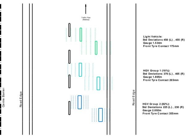
Using the average position and standard deviation data, it was possible to plot the front tyres average position and extent of lateral wander for the three vehicle categories. The scaled drawing example below (figure 4) shows average front tyre position (full lines) and one, two and three standard deviations (intermittent lines) for each vehicle category.

Figure 4. Tyre position distribution – E4 Motorway, Linköping.

In this example (figure 4), it can be seen that the offside (left hand side) tyre average position was similar for all three vehicle groups. This suggests that, for motorway type roads, maximum rutting will occur in the offside tyre track if the road structure has uniform resistance against surface wear and deformation. The rut is also likely to have a near symmetrical shape. On the nearside (right hand side), tyre positions were not the same. This is likely to result in an unsymmetrical rut shape being formed with the maximum rut depth occurring in the HGV group 2 position. The overlapping that occurs between the offside and nearside tyres (light vehicles and HGV Group 1 only) will also have some effect on rut formation.

The suggestion can be confirmed by examining the cross section profile at the surveyed location (figure 5). Rut development is discussed further in chapter 4.8.

150 3700 2600 ? ? K2 K1 R o a d E d g e C e n tr e B a rr ie r R o a d E d g e HGV Grou p 1 (18 %): Std Devia tions 370 (L ) , 405 (R) Gau ge 1.8 05m

Fro nt Tyr e Cont act 26 5mm

Traffic Flow (Mantorp)

Verge

Lig ht V ehic le:

Std Dev iation s 450 (L) , 455 (R) Gau ge 1.5 34m Fro nt Ty re C ontac t 175 mm HG V Gr oup 2 (82% ): Std Devia tions 225 (L ) , 230 (R) Gau ge 2.0 92m Fro nt Ty re C ontac t 355 mm

(22)

Figure 5. Actual Cross Section Profile - E4 Motorway at Ref 5b (Trafikverket PMSv3).

3.5. Position survey locations

The Swedish national road network can be divided into groups depending on category and type. The tables below show road lengths and usage (vehicle kilometres) in 2015.

Table 1. State and Local Authority Maintained Roads (trafikverket.se).

Road Km Vehicle km (milliard km)

State Maintained 98,500 58

Local Authority Maintained 42,200 24

Table 2. Road Category 2015 (trafikverket.se).

Category Km Vehicle km (milliard km)

European Route 6,700 23 (40%)

National Route 8,900 14 (24%)

Primary Rural Road 10,800 9 (16%)

Other Rural Road 72,100 12 (20%)

Total 98,500 58

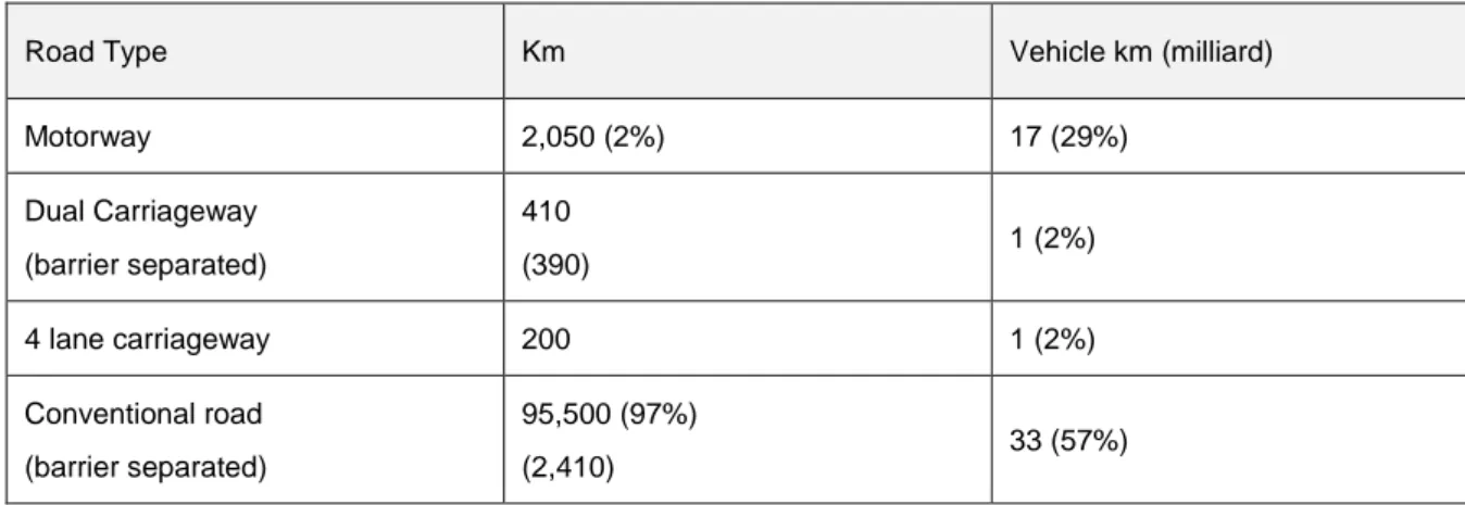
Table 3. Road Type 2015 (trafikverket.se).

Road Type Km Vehicle km (milliard)

Motorway 2,050 (2%) 17 (29%) Dual Carriageway (barrier separated) 410 (390) 1 (2%) 4 lane carriageway 200 1 (2%) Conventional road (barrier separated) 95,500 (97%) (2,410) 33 (57%)

Only around 2% of the national road network is constructed to motorway standard. However, approximately 29% of all vehicle traffic is carried on this type of road. On the other hand, conventional road types make up 97% of the road network and carry 57% of traffic. Position surveys were carried out on a selection of the above road types.

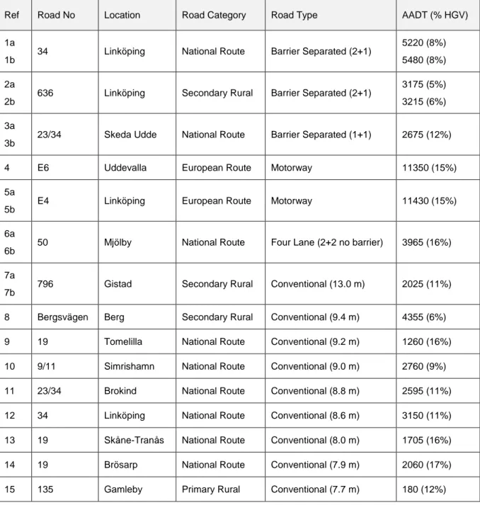
Position surveys were carried out at the fifteen locations detailed in Table 4. Twenty-one surveys provided data on approximately 271,000 vehicles.

(23)

Table 4. Position Survey Locations.

Ref Road No Location Road Category Road Type AADT (% HGV) 1a

1b 34 Linköping National Route Barrier Separated (2+1)

5220 (8%) 5480 (8%) 2a

2b 636 Linköping Secondary Rural Barrier Separated (2+1)

3175 (5%) 3215 (6%) 3a

3b 23/34 Skeda Udde National Route Barrier Separated (1+1) 2675 (12%) 4 E6 Uddevalla European Route Motorway 11350 (15%) 5a

5b

E4 Linköping European Route Motorway 11430 (15%)

6a

6b 50 Mjölby National Route Four Lane (2+2 no barrier) 3965 (16%) 7a

7b 796 Gistad Secondary Rural Conventional (13.0 m) 2025 (11%) 8 Bergsvägen Berg Secondary Rural Conventional (9.4 m) 4355 (6%) 9 19 Tomelilla National Route Conventional (9.2 m) 1260 (16%) 10 9/11 Simrishamn National Route Conventional (9.0 m) 2760 (9%) 11 23/34 Brokind National Route Conventional (8.8 m) 2595 (11%) 12 34 Linköping National Route Conventional (8.6 m) 3150 (11%) 13 19 Skåne-Tranås National Route Conventional (8.0 m) 1705 (16%) 14 19 Brösarp National Route Conventional (7.9 m) 2060 (17%) 15 135 Gamleby Primary Rural Conventional (7.7 m) 180 (12%)

(24)

4. Results and discussion

A summary of the amount of vehicular lateral wander (standard deviation of average position) is provided in the following table. The sample size (number of recorded vehicles) for each survey is also stated.

Table 5. Vehicular Lateral Wander and Sample Size.

Further information on cross section dimensions, distribution of lateral position, average lateral position, variation of lateral position, and vehicle tracking is provided in Appendix 2.

Left Right Left Right Left Right

1a 34 2+1 270 270 245 250 215 215 41766 1b 34 2+1 375 375 290 325 225 225 22523 2a 636 2+1 255 260 225 225 190 185 30610 2b 636 2+1 400 400 265 305 260 270 25871 3a 23/34 1+1 190 195 195 190 140 150 6998 3b 23/34 1+1 200 200 195 190 150 145 7740 4 E6 Motorway 380 365 310 330 255 255 24142 5a E4 Motorway 450 455 370 405 225 230 8452 5b E4 Motorway 405 405 315 355 220 220 18118 6a 50 Four Lane 270 265 250 270 220 220 3658 6b 50 Four Lane 270 280 235 285 215 225 4149 7a 796 Conventional 355 355 410 425 395 380 12796 7b 796 Conventional 400 400 410 425 430 415 4475 8 Bergsvägen Conventional 315 315 300 300 285 260 20074 9 19 Conventional 350 355 290 325 240 240 3383 10 9/11 Conventional 375 380 360 375 270 275 6165 11 23/34 Conventional 320 310 295 305 240 215 9079 12 34 Conventional 300 295 265 280 205 210 12251 13 19 Conventional 300 300 250 285 195 195 4400 14 19 Conventional 315 315 260 265 210 215 4290 15 135 Conventional 265 270 305 300 260 240 754 Total 271694 Max 450 455 410 425 430 415 Min 190 195 195 190 140 145

Ref Road No Road Type HGV1 HGV2 Sample Size _(vehicles)

Std Dev (mm) Light Vehicle

(25)

4.1. Standard deviations of average position

As previously mentioned in Chapter 3.3, the three sigma rule states that nearly all values will be contained within three standard deviations of the mean. By applying this rule, it can be assumed that nearly all tyre positions will be contained within three standard deviations of the average tyre position. The standard deviation of a vehicle’s position is a good indicator of the variation in lateral position. In the following figure, standard deviation values have been plotted for the offside tyres of three main groups of vehicles:

 light vehicles (1.5 m track width),  HGV Group 1 (1.8 m track width), and  HGV Group 2 (2.1 m track width).

Figure 6. Lateral Wander per Road Type and Vehicle Group.

In the majority of the results, vehicles with smaller axle track widths tended to have more lateral wander. The exceptions were at locations 7 and 15.

Traffic observations at location 7 revealed that slower, heavier vehicles tended to move into the 2.8 m wide side verge to allow faster vehicles to over-take. This could help explain the higher lateral wander values associated with the HGV groups.

The observed order of the variation for different vehicle categories at location 15 differs from other locations with similar properties. Traffic volume at location 15 was very low, however, a statistical test showed that the variation for HGV1 was not significantly greater than that for light vehicles. It cannot be rejected that the order should in fact be the same as in locations 8 to 14.

Conventional 2+2

M’way 1+1

(26)

4.2. 2+1 road type

With regard to “2+1” road types, Figure 7, clear differences in the amount of lateral wander can be seen between the single lane sections (ref 1a and 2a) and the double lane sections (ref 1b and 2b).

Figure 7. Lateral Wander Comparisons – “2+1” Road.

It is therefore assumed that road degradation rates in the single lane sections will be higher than in the double lane sections. This can be confirmed by analysing rut depth and traffic volume data obtained from the Swedish Road Administrators (Trafikverket) PMSv3 database – Figure 8.

(27)

4.3. Conventional road converted to “1+1” barrier separated road

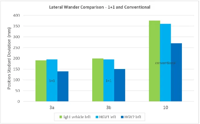
Comparisons between reference 3a and 3b (9 m wide 1+1 barrier separated) and reference 10 (9 m wide conventional road) show that lateral wander is much lower on the barrier separated road layout.

Figure 9. Lateral Wander Comparisons – 9 m “1+1” with 9m Conventional Road.

Figure 9 illustrates the considerable reduction in vehicle lateral wander that occurs when a 9 m wide conventional road is converted into a 9 m wide “1+1” barrier separated road.

Reference 3a and 3b were converted to a barrier separated road in 2011 and partly resurfaced during 2014. Insufficient road surface survey data meant that it was not possible to compare rut development rates before and after the conversion.

However, the fact that resurfacing work was required three years after conversion, may give an indication of how severe confinement of traffic can accelerate degradation rates.

(28)

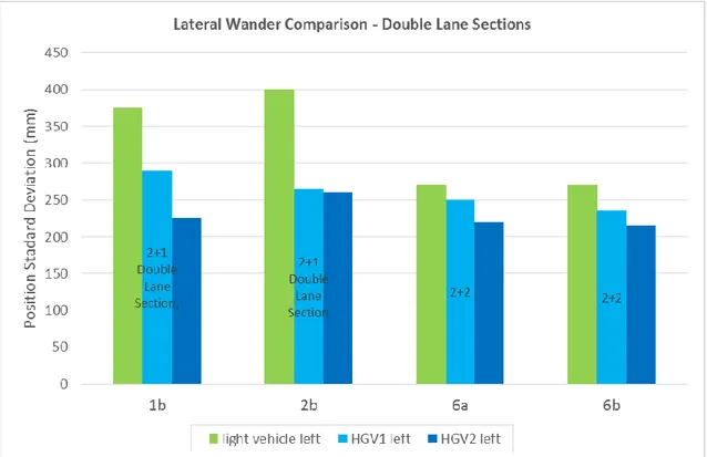
4.4. Double lane sections

Lateral wander values for light vehicles on a “2+2” road type (ref 6a and 6b) were considered to be quite low. These should have been comparable with values on the double lane sections of a “2+1” road type (ref 1b and 2b).

A possible explanation for this is that the narrower side verge, associated with ref 6, may have had some confining effect on the amount of lateral wander.

(29)

4.5. Effect of lane type and side verge widths

Figure 11. Lateral Wander, Lane Widths, and Side Verge Widths.

Regarding “2+1” and motorway road types (reference 1b, 2b, 4, 5a and 5b), the presence of the adjacent second lane is likely to have a positive effect and increase the amount of lateral wander. For motorway road types (reference 4, 5a and 5b), the presence of a wide side verge is also likely to have influenced the higher values associated with light vehicle and HGV Group 1 values.

The effect of a wide side verge can also be seen in conventional road types 7a and 7b.

Conventional 2+2

M’way 1+1

(30)

4.6. Narrow lane and side verge widths

The very low lateral wander values associated with the “1+1” sections (ref 3a and 3b) can be attributed to narrower lane widths and the close proximity of the central barrier.

Figure 12. Single Lane Section Comparisons – 1+1 and 2+1 Road Types.

With regard to reference 3a and 3b, lane widths were found to be narrower. In addition, the distance from the offside lane edge marking to the central barrier was only 400 mm. The same dimension in comparable road types, reference 1a and 2a, was 800 mm and 1100 mm respectively.

(31)

4.7. Lateral wander and lane widths

With reference to conventional road types, the following figure shows trends between the amount of lateral wander and the widths of lanes and side verges.

Figure 13. Conventional Road Types – Lateral Wander and Lane Widths.

With the exception of references 7a, 7b and 15, there is a connection between lane width and the amount of vehicle lateral wander – especially with the HGV Group 2 category.

The wide side verges associated with reference 7a and 7b have probably contributed to the high amount of lateral wander.

As stated previously in Chapter 4.1, traffic volume at reference 15 was very low. Variations for HGV1 were not significantly greater than that for light vehicles and it cannot be rejected that the order should in fact be the same as in locations 8 to 14.

(32)

4.8. Rut development rates

Vehicle position is a factor that has an influence on rut formation. An example of this can be demonstrated in Figure 14. The approximate positions of Light Vehicles, HGV Group 1, and HGV Group 2 have been added to the cross section profile previously detailed in Chapter 3.4.

Figure 14. Actual Cross Section Profile - E4 Motorway at Ref 5b (Trafikverket PMSv3).

The figure shows two different types of rut formation. On the vehicles offside, surface wear and deformation is confined to a deeper, narrower, symmetrical type of rut. The nearside rut is much wider and not as deep – surface wear and deformation are not confined to the same track.

Using data extracted from the Swedish Road Administrators (Trafikverket) PMSv3 Database, it was possible to calculate rut development rates and traffic volumes for the examples shown below in Figure 15. Due to insufficient data, it was not possible to calculate rates for references 3, 6 and 7. Reference 4 formed part of a test road so rates were considered not to be comparable. Results show that in every case, development rates were higher in the left hand side rut.

(33)

5. Conclusions and further work

Vehicle position and amount of vehicular lateral wander will have an effect on the rate of pavement wear. Pavements will deteriorate at a quicker rate where lateral wander is constricted by a confining design.

A method to determine the lateral position of a vehicle has been used to provide vehicle position data on a range of common road types found on the Swedish road network. Twenty-one sets of survey data provided information on over 271,000 vehicles. The information was split into three vehicle groups depending on the axle track width.

Using the survey data, it was possible to calculate and plot the distribution of lateral position, the average position, and the variation of lateral position (lateral wander) for each group. In order to try and determine the distribution of wheel paths, the centre point of a single or double wheel,

development work on the “Z” measuring system is being carried out (McGarvey, 2016) so that tyre widths and types can also be determined.

Factors such as lane type, lane width, verge width, total width, and close proximity of guardrail all had some influence on vehicle position and amount of lateral wander.

The extent of lateral wander varied quite considerably. Values associated with light vehicles varied between 455 mm and 190 mm. Commercial traffic values were lower and ranged between 430 mm and 140 mm. These are significant variations and should be considered when planning reconstruction or maintenance work.

The information contained in this report may prove to be very useful when trying to interpret road surface characteristic data recorded in databases such as Trafikverkets PMSv3. It may also prove useful when calculating rates of surface wear and deformation in prediction models such as VTIs Surface Wear Model (Wågberg och Jacobson, 2007) and PEDRO (Oscarsson & Said, 2011). The information may also be important for tyre/pavement rolling resistance research where rolling resistance indicators use measured road condition characteristics. The results can be used to help guide where in the road these characteristics should be measured.

Around forty different types of vehicle were identified by the measurement system. If required, it is possible to study the position and behaviour of a particular type of vehicle.

Surveys were carried out on relatively straight, open road sections. It is possible that vehicle position and amount of lateral wander will be affected by road curvature and surroundings. The extent of these effects is unknown and may warrant further investigation.

(34)

(35)

References

McGarvey, T (in progress), Barrier separated road type design - accelerated degradation, VTI Rapport, Swedish national road and transport research institute, Linköping

Carlsson, A (2009), Uppföljning av mötesfria vägar – Slutrapport. VTI Rapport 636, Swedish national road and transport research institute, Linköping

Anund, P och Sörensen, G (1995), PREC95, ett program för bearbetning och analys av

trafikmätningsdata: Beskrivning och manual, VTI Notat T147, Swedish national road and transport

research institute, Linköping

Wågberg Lars-Göran och Jacobson Torbjörn (1997), Utveckling av prognosmodell för

beläggningsslitage, slitageprofil och årsmodell. VTI Notat 21, Swedish national road and transport

research institute, Linköping

Wågberg Lars-Göran och Jacobson Torbjörn (2007), Utveckling och uppgradering av prognosmodell

för beläggningsslitage från dubbade däck samt en kunskapsöversikt över inverkande faktorer. VTI

Notat 7, Swedish national road and transport research institute, Linköping

Oscarsson, E. & Said, S. (2011), Modelling Permanent Deformations in Asphalt Concrete Layers

Using the PEDRO Model.

McGarvey, T (2016), Measurement of tyre width and assembly type (single or double tyre), VTI Rapport 899, Swedish national road and transport research institute, Linköping

(36)

(37)

Appendix 1

It was possible to split HGV’s into two groups depending on vehicle track width. HGV’s classified as vehicle code“22” had an average axle track width of 1.805m and, in the case below, accounted for 18% of all HGV traffic.

Road E4 (motorway) near Linköping:

(38)

(39)

Appendix 2

Ref 1a: Road 34, Linköping, National Route, Barrier Separated (2+1)

(40)

Tyre tracking, assuming the following front tyre contact (with road surface) widths:  light vehicles – 205 size = 175 mm surface contact width,

 HGV Group 1 – 295 size = 265 mm surface contact width, and

 HGV Group 2 – 385 size = 355 mm contact surface width.

Figure 18. Ref 1a – Tyre Tracking in Single Lane Section.

Photograph 3. Ref 1a. (Photo. Terence McGarvey).

C e n tr e G a u rd ra il (Linköping) (Linköping)

(41)

Ref 1b: Road 34, Linköping, National Route, Barrier Separated (2+1)

Figure 19. Ref 1b – Distribution of Lateral Position.

(42)

Figure 21. Ref 1b – Tyre Tracking in Double Lane Section.

Photograph 4. Ref 1b. (Photo. Terence McGarvey).

C e n tr e G a u rd ra il (Motala)

(43)

Ref 2a: Road 636, Linköping, Secondary Rural Road, Barrier Separated (2+1)

(44)

Figure 24. Ref 2a – Tyre Tracking in Single Lane Section.

C e n tr e G a u rd ra il (Linköping) Traffi c Flow (Linköping) Traffi c Flow

(45)

Ref 2b: Road 636, Linköping, Secondary Rural Road, Barrier Separated (2+1)

(46)

Figure 27. Ref 2b – Tyre Tracking in Double Lane Section.

C e n tr e G a u rd ra il Traffi c Flow (Vikingstad)

(47)

Ref 3a: Road 23/34, Skeda Udde, National Route, Barrier Separated (1+1)

Figure 28. Ref 3a – Distribution of Lateral Position.

(48)

Figure 30. Ref 3a – Tyre Tracking.

Photograph 7. Ref 31. (Photo. Terence McGarvey).

Traffi c Flow (Linköping)

(49)

Ref 3b: Road 23/34, Skeda Udde, National Route, Barrier Separated (1+1)

(50)

Figure 33. Ref 3b – Tyre Tracking.

Traffi c Flow (Brokind))

(51)

Ref 4: E6, Uddevalla, European Route, Motorway

Figure 34. Ref 4 Distribution of Lateral Position.

(52)

Figure 36. Ref 4 – Tyre Tracking.

Photograph 9. Ref 4. (Photo. Terence McGarvey).

R o a d E d g e C e n tr e B a rr ie r R o a d E d g e

(53)

Ref 5a: E4, Linköping, European Route, Motorway

(54)

Figure 39. Ref 5a - Tyre Tracking.

Photograph 10. Ref 5a. (Photo. Trafikverket PMSv3).

R o a d E d g e C e n tr e B a rr ie r R o a d E d g e Traffi c Flow (Mantorp)

(55)

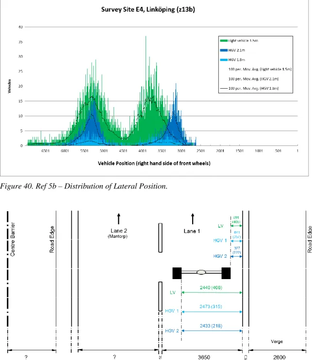
Ref 5b: E4, Linköping, European Route, Motorway

(56)

Figure 42. Ref 5b - Tyre Tracking.

Photograph 11. Ref 5b. (Photo. Trafikverket PMSv3).

R o a d E d g e C e n tr e B a rr ie r R o a d E d g e Traffi c Flow (Mantorp)

(57)

Ref 6a: Road 50, Mjölby, National Route, Four Lane

(58)

Mjölby C e n tr a l R e s e rv e

(59)

Ref 6b: Road 50, Mjölby, National Route, Four Lane

(60)

Motala C e n tr a l R e s e rv e

(61)

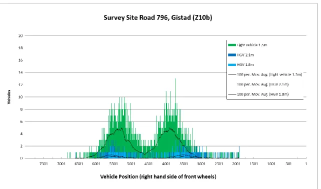
Ref 7a: Road 796, Gistad, Secondary Rural Road, Standard (13.35 m)

Figure 49. Ref 7a - Distribution of Lateral Position.

(62)

(63)

Ref 7b: Road 796, Gistad, Secondary Rural Road, Standard (13.35 m)

(64)

(65)

Ref 8: Bergsvägen, Berg, Secondary Rural Road, Standard (9.4 m)

Figure 55. Ref 8 – Distribution of Lateral Position.

(66)

Figure 57. Ref 8 - Tyre Tracking.

Photograph 16. Ref 8. (Photo. Håkan Wilhelmsson).

V e rg e R o a d e d g e

(67)

Ref 9: Road 19, Tomelilla, National Route, Standard (9.2 m)

(68)

(69)

Ref 10: Road 9/11, Simrishamn, National Route, Standard (9.0 m)

(70)

(71)

Ref 11: Road 23/34, Brokind, National Route, Standard (8.8 m)

(72)

(73)

Ref 12: Road 34, Linköping, National Route, Standard (8.6 m)

(74)

(75)

Ref 13: Road 19, Skåne - Tranås, National Route, Standard (8.0 m)

(76)

(77)

Ref 14: Road 19, North of Brösarp, National Route, Standard (7.9 m)

(78)

(79)

Ref 15: Road 135, Gamleby, Primary Rural Road, Standard (7.7 m)

(80)

(81)

(82)

www.vti.se

VTI, Statens väg- och transportforskningsinstitut, är ett oberoende och internationellt framstående forskningsinstitut inom transportsektorn. Huvuduppgiften är att bedriva forskning och utveckling kring

infrastruktur, trafi k och transporter. Kvalitetssystemet och

miljöledningssystemet är ISO-certifi erat enligt ISO 9001 respektive 14001. Vissa provningsmetoder är dessutom ackrediterade av Swedac. VTI har omkring 200 medarbetare och fi nns i Linköping (huvudkontor), Stockholm, Göteborg, Borlänge och Lund.

The Swedish National Road and Transport Research Institute (VTI), is an independent and internationally prominent research institute in the transport sector. Its principal task is to conduct research and development related to infrastructure, traffi c and transport. The institute holds the quality management systems certifi cate ISO 9001 and the environmental management systems certifi cate ISO 14001. Some of its test methods are also certifi ed by Swedac. VTI has about 200 employees and is located in Linköping (head offi ce), Stockholm, Gothenburg, Borlänge and Lund.

HEAD OFFICE LINKÖPING SE-581 95 LINKÖPING PHONE +46 (0)13-20 40 00 STOCKHOLM Box 55685 SE-102 15 STOCKHOLM PHONE +46 (0)8-555 770 20 GOTHENBURG Box 8072 SE-402 78 GOTHENBURG PHONE +46 (0)31-750 26 00 BORLÄNGE Box 920 SE-781 29 BORLÄNGE PHONE +46 (0)243-44 68 60 LUND Medicon Village AB SE-223 81 LUND PHONE +46 (0)46-540 75 00

Vehicle lateral position depending on road type and lane width : vehicle position surveys carried out on the Swedish road network

Terence McGarvey

Vehicle lateral position depending on

road type and lane width

Vehicle position surveys carried out

on the Swedish road network

VTI rapport 892A

Published 2016

VTI rapport 892A

Vehicle lateral position depending on road

type and lane width

Vehicle position surveys carried out

on the Swedish road network

Abstract

Referat

Foreword

Quality review

Kvalitetsgranskning

Contents

Summary

Sammanfattning

1.

Introduction

2.

Aim

3.

Method

3.1.

Measurement technique

3.2.

Distribution of lateral position (right hand side of front tyres)

3.3.

Average position and standard deviations

3.4.

Tyre tracking

3.5.

Position survey locations

4.

Results and discussion

4.1.

Standard deviations of average position

4.2.

2+1 road type

4.3.

Conventional road converted to “1+1” barrier separated road

4.4.

Double lane sections

4.5.

Effect of lane type and side verge widths

4.6.

Narrow lane and side verge widths

4.7.

Lateral wander and lane widths

4.8.

Rut development rates

5.

Conclusions and further work

References

Appendix 1

Appendix 2

www.vti.se