Shahrooz Abghari
1 a, Veselka Boeva
1, Jens Brage
2and H˚akan Grahn
1 b1Department of Computer Science, Blekinge Institute of Technology, Karlskrona, Sweden 2NODA Intelligent Systems AB, Karlshamn, Sweden
Keywords: Data Mining, Multi-view Clustering, Multi-layer Clustering, Time Series, District Heating Substation. Abstract: In this study, we propose a multi-view clustering approach for mining and analysing multi-view network
datasets. The proposed approach is applied and evaluated on a real-world scenario for monitoring and analysing district heating (DH) network conditions and identifying substations with sub-optimal behaviour. Initially, geographical locations of the substations are used to build an approximate graph representation of the DH network. Two different analyses can further be applied in this context: step-wise and parallel-wise multi-view clustering. The step-wise analysis is meant to sequentially consider and analyse substations with respect to a few different views. At each step, a new clustering solution is built on top of the one generated by the previously considered view, which organizes the substations in a hierarchical structure that can be used for multi-view comparisons. The parallel-wise analysis on the other hand, provides the opportunity to analyse substations with regards to two different views in parallel. Such analysis is aimed to represent and identify the relationships between substations by organizing them in a bipartite graph and analysing the substations’ distribution with respect to each view. The proposed data analysis and visualization approach arms domain experts with means for analysing DH network performance. In addition, it will facilitate the identification of substations with deviating operational behaviour based on comparative analysis with their closely located neighbours.
1
INTRODUCTION
District heating (DH) systems utilize hot water and heat produced at a production unit for a number of consumer units, i.e., buildings, in a limited geograph-ical area through a distribution network. This part of the system is referred to as the primary side. The con-sumer unit itself consists of a heat exchanger, a circu-lation network, and radiators for the rooms, which are considered as the secondary side. The primary and secondary sides are connected together through a sub-station, which is responsible for adjusting the pressure and the temperature of the supply water suitable for the consumer unit.
In the DH domain, energy companies need to ad-dress several conflicting goals such as satisfying con-sumers’ heat demand including domestic hot water (DHW) while minimizing production and distribu-tion costs. Such complexity demands fault detecdistribu-tion and root cause analysis techniques for identification of deviating behaviours and faults. Undetected faults
a https://orcid.org/0000-0002-3010-8798 b https://orcid.org/0000-0001-9947-1088
can lead to underlying problems, which in return can increase the maintenance cost and reduce the con-sumers’ satisfaction. When it comes to monitoring of a DH network there are different features and char-acteristics that one needs to consider. Domain experts often analyse substations individually or in a group with regard to one specific feature or a combination of features. While this provides useful information for the whole network it does not take into account the location of the substations along the distribution network and their neighbouring substations automat-ically. In other words, the operational behaviours of the DH substations need to be assessed jointly with surrounding substations within a limited geographi-cal distance. Due to the nature of the data and the fact that different data representations can be used, the process of monitoring and identifying faults and de-viating behaviours of the DH system and substations can be treated as a multi-view data analysis problem.
Multi-view datasets consist of multiple data repre-sentations or views, where each one may contain sev-eral features (Deepak and Anna, 2019). Multi-view learning is a semi-supervised approach with the goal
158
Abghari, S., Boeva, V., Brage, J. and Grahn, H.
Multi-view Clustering Analyses for District Heating Substations. DOI: 10.5220/0009780001580168
to obtain better performance by applying the relation-ship between different views rather than one to facil-itate the difficulty of a learning problem (Blum and Mitchell, 1998; Ando and Zhang, 2007; Xu et al., 2013). Due to availability of inexpensive unlabeled data in many application domains, multi-view unsu-pervised learning and specifically multi-view cluster-ing (MVC) attract great attention (Deepak and Anna, 2019). The goal of multi-view clustering is to find groups of similar objects based on multiple data rep-resentations.
We propose a multi-view clustering analysis ap-proach for mining network datasets with multiple rep-resentations. The proposed approach is used for mon-itoring a DH network and identifying DH substa-tions with sub-optimal operational behavior. We ini-tially use geographical location of substations to di-vide them into groups of similar substations based on their distance and location. In that way, we are able to: 1) group the substations (network nodes) based on their location and distance, 2) build an approx-imate graph representation of the DH network, and 3) order the substations using information about the DH network structure and the average supply water temperature for a specific period. Two different types of analyses can then be applied in this scenario: i) step-wise clustering to sequentially consider and anal-yse substations with respect to a few different views; ii) parallel-wise clustering to analyse substations with regards to two different views in parallel.
2
RELATED WORK
MVC clustering algorithms have been proposed based on different frameworks and approaches such as k-means variants (Bickel and Scheffer, 2004; Cai et al., 2013; Jiang et al., 2016), matrix factorization (Liu et al., 2013; Zong et al., 2017), spectral methods (Ku-mar and Daum´e, 2011; Wang et al., 2013) and exemplar-based approaches (Meng et al., 2015; Wang et al., 2015).
Bickel and Scheffers (Bickel and Scheffer, 2004) proposed extensions to different partitioning and ag-glomerative MVC algorithm. That study can proba-bly be recognized as one of the earliest works where an extension of k-means algorithm for two-view doc-ument clustering is proposed. In another study (Cai et al., 2013), the authors developed a large-scale MVC algorithm based on k-means with a strategy for weighting views. The proposed method is based on the `2,1 norm, where the `1norm is enforced on data
points to reduce the effect of outlier data and the `2
norm is applied on the features. In a recent study,
Jiang et al. (Jiang et al., 2016) proposed an extension of k-means with a strategy for weighting both views and features. Each feature within each view is given bi-level weights to express its importance both at the feature level and the view level.
Liu et al. (Liu et al., 2013) proposed an MVC algorithm based on joint non-negative matrix factor-ization (NMF). The developed algorithm incorporates separate matrix factorizations to achieve similar coef-ficient matrices and further meaningful and compara-ble clustering solution across all views. In a recent study, Zong et al. (Zong et al., 2017) proposed an ex-tension of NMF for MVC that is based on manifold regularization. The proposed framework maintains the locally geometrical structure of multi-view data by including consensus manifold and consensus coef-ficient matrix with multi-manifold regularization.
Kumar and Daum´e (Kumar and Daum´e, 2011) proposed an MVC algorithm for two-view data by combining co-training and spectral clustering. The approach is based on learning the clustering in one view to label the data and modify the similarity ma-trix of the other view. The modification of the sim-ilarity matrices are performed using discriminative eigenvectors. Wang et al. (Wang et al., 2013) pro-posed a variant of spectral MVC method for situations where there are disagreements between data views us-ing Pareto optimization as a means of relaxation of the agreement assumption.
Meng et al. (Meng et al., 2015) proposed an MVC algorithm based on affinity propagation (AP) for sci-entific journal clustering where the similarity matrices of the two views (text view and citations view) are in-tegrated as a weighted average similarity matrix. In another study, Wang et al. (Wang et al., 2015) pro-posed a variant of AP where an MVC model consists of two components for measuring 1) the within-view clustering quality and 2) the explicit clustering con-sistency across different views.
Fault detection and diagnosis (FDD) is an active field of research and has been studied in different application domains. Isermann (Isermann, 1997; Is-ermann, 2006) provided a general review for FDD. Katipamula and Brambley (Katipamula and Bramb-ley, 2005a; Katipamula and BrambBramb-ley, 2005b) con-ducted an extensive review in two parts on fault de-tection and diagnosis for building systems. Xue et al. (Xue et al., 2017) applied clustering analysis and association rule mining to detect faults in substations. Sandin et al. (Sandin et al., 2013) used probabilistic methods and heuristics for automated detection and ranking of faults in large-scale district energy sys-tems. Calikus et al. (Calikus et al., 2019) proposed an approach for automatically 1) discovering heat load
patterns in DH systems and 2) identifying buildings with abnormal heat profiles and unsuitable control strategies.
In contrast to the above mentioned methods, this study proposes a multi-view data analysis approach that can be applied for monitoring, evaluating and visualizing the operational behaviour of DH substa-tions. The geographical location data is used as a backbone of the analysis and the operational perfor-mance of the substations is further assessed in con-junction with their neighbours.
3
PROBLEM FORMALIZATION
We have a network with N nodes, e.g., a DH network linking a set of substations located in some geograph-ical region. Assume that each network node, substa-tion, i (i = 1, 2, . . . , N) is monitored under n differ-ent conditions (i.e., the measuremdiffer-ents of n differdiffer-ent features are collected) for a given time period, e.g., mdays. Each monitored condition j ( j = 1, 2, . . . , n) contains the measured levels of the corresponding fea-ture for a period of m days in t different time points. This leads to a set of n time series data matrices Dj
( j = 1, 2, . . . , n), one per feature, for each network node.
This multi-view data context can additionally be complicated in the case of a real-world scenario such as one related to a DH network. For example, the operational behaviour of the substations varies dur-ing heatdur-ing and non-heatdur-ing seasons which requires separate analysis. Therefore, for each substation two datasets are usually collected and available for further analysis and comparison. Notice that in this study, we are only interested in the operational behaviour of the DH substations during heating season due to the importance of space heating.
The main challenge in the above multi-view con-text is how to use all available measurements about the substations’ operational behaviour and perfor-mance for better understanding and improved main-tenance of the DH network. Exploiting the whole po-tential of these real-world datasets is not trivial and it requires suitable data analysis techniques to prevent information loss.
4
METHODS
4.1
Clustering Analysis
In this study, we are interested in identifying homoge-neous groups of substations by considering their
loca-tions and additionally analysing them with respect to different views (features). Due to unavailability of the labeled data, clustering analysis is applied to explore hidden structures within the data. We apply two clus-tering algorithms as follows:
1. Minimum Spanning Tree Clustering: We use Van-derPlas’ (VanderPlas, 2016) Python implantation of the minimum spanning tree (MST) clustering algo-rithm for grouping substations based on their geo-graphical location. The algorithm is based on con-structing an approximate Euclidean minimum span-ning tree (EMST), which considers only k nearest neighbours of each point for building the minimum spanning tree rather than the entire set of edges in a complete graph.
2. Affinity Propagation: We use the affinity prop-agation (AP) algorithm (Frey and Dueck, 2007) for clustering the time series based on their similarities. AP works based on the concept of message pass-ingbetween data points to first identify a suitable set of exemplars and then to choose which data points should pick which exemplars. One of the advantages of AP, unlike other clustering algorithms, such as k-means (MacQueen et al., 1967) which requires the number of clusters as an input, is that it estimates the optimal number of clusters from the data. In addition, the chosen exemplars, the representative of the clus-ters, are real data points which makes AP a suitable clustering algorithm for this study.
4.2
Similarity Measures
We use different similarity measures, 1) to check the similarity between daily time series profiles of each feature, 2) to perform pairwise comparison between exemplars of clustering solutions of different substa-tions, and 3) to compute a similarity between two clustering solutions by considering all pairs of mem-bers. These similarity measures are as follows: 1. Dynamic Time Warping: Given two time series Y = (y1, y2, ..., yn) and Y0= (y01, y02, ..., y0m), the
simi-larity between Y and Y0can be measured using the dy-namic time warping (DTW) algorithm. DTW is pro-posed by Sakoe and Chiba (Sakoe and Chiba, 1978) for spoken word detection with the focus of eliminat-ing timeliminat-ing differences between two speech patterns. In other words, DTW identifies an optimal match-ing between the given sequences by warpmatch-ing the time axis. In order to align the time series Y and Y0 of length n and m respectively, a cost matrix, Qn×mis
computed. Each element, qi j, of Qn×mcorresponds
to the distance (often Euclidean) between yiand y0jof
the two series. Using the cost matrix, the DTW tries to find the best alignment path between these two time
series that is leading to minimum overall cost. The best warping path should satisfy a different number of conditions such as monotonicity, continuity, bound-ary, warping window, and slope constraint.
2. Clustering Solution Similarities: Given two clustering solutions C = {C1,C2, . . . ,Cn} and C0 =
{C10,C02, . . . ,Cm0} of datasets X and X0, respectively, the similarity, CSw, between C and C
0can be assessed
as follows (Abghari et al., 2019):
CSw(C,C 0) =∑ n i=1(minmj=1wi.d(ci, c0j)) 2 + ∑mj=1(minni=1w0j.d(ci, c0j)) 2 , (1)
where ciand c0j are exemplars of the clustering
solu-tion Ciand C0j, respectively. The weights wiand w0j
indicate the relative importance of clusters Ciand C0j
compared to other clusters in the clustering solution Cand C0, respectively. For example, a weight wi of
a cluster Cican be calculated as the ratio of its
cardi-nality with respect to the size of X , i.e., wi= |Ci|/|X|.
The CSwhas values in a range of [0,1]. Scores equal to zero imply identical performance while scores close to one show significant dissimilarities.
3. Adjusted Rand Index: The quality of the results of a clustering analysis can be validated by means of in-ternaland external criteria. Internal criteria evaluate the quality of the clustering solution produced by a clustering algorithm that fits the data in terms of, e.g., compactness and separation by using the inherent in-formation of the data. External criteria on the other hand, can be used for measuring the level of agree-ments between the results of a clustering algorithm in comparison with ground truth, the results of another clustering algorithm on the same data, or same clus-tering algorithm but by considering different views.
In this study, we apply a symmetric external val-idation index for assessing the similarity (consen-sus) between two clustering results generated on the studied DH substations with respect to two differ-ent views. The adjusted Rand index (ARI) (Hubert and Arabie, 1985) is a correction of the Rand in-dex (RI) (Rand, 1971) that measures the similarity between two clustering solutions by considering the level of agreements between the two groups. ARI is computed as follows:
ARI= RI− ExpectedRI
Max(RI) − ExpectedRI (2) ARI scores are bound between -1 and +1. A score less than or equal to 0 represents random labelling and 1 stands for perfect match.
5
PROPOSED APPROACH
Geographical locations of N substations are initially used for building an approximate graph representa-tion of the DH network. We refer to the geograph-ical location of the substations as the Location view (v0). This is performed by applying the MST
cluster-ing algorithm described in Section 4. The aim is to connect substations based on their distance by build-ing a minimum spannbuild-ing tree and removbuild-ing edges of the tree with regard to a cut-off threshold. Therefore, each cluster is represented by a tree that can be in-terpreted as a representation of the DH network struc-ture. In order to provide additional support for the do-main experts, the graph representation can in turn be used as a backbone for additional information about the DH network, e.g., average yearly values and dif-ferent forms of ranking.
On the foundation of the created grouping of the substations we can perform further analysis by focus-ing on a specific feature or subset of features and eval-uate the substations’ operational behaviours in each single location-based cluster. We study and evaluate the following two scenarios:
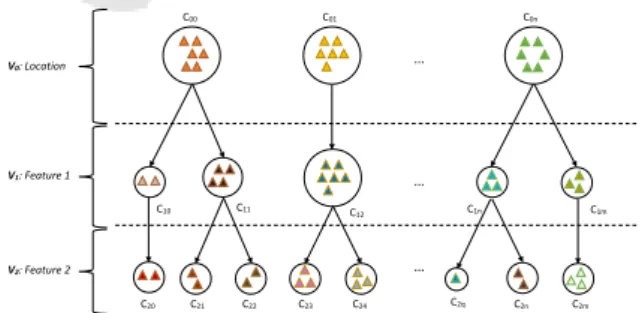
1. Step-wise multi-view clustering (SW-MVC), we can apply clustering analysis on substations that have been grouped together at the previous step with re-spect to a set of features, i.e., the substations can be grouped by considering one feature at a time. This scenario can be used when the domain experts are in-terested in grouping similar substations based on their performance with respect to one feature and then find-ing similar substations in each group by usfind-ing another feature and so on. Figure 1 shows how the results of this analysis can be visualized based on the location of the substations and two features.
C1m C12 C11 C1n C10 C00 C01 C0n … … … C20 C21 V0: Location V1: Feature 1 C22 C23 C24 C2q C2n C2m V2: Feature 2
Figure 1: SW-MVC analysis, each view represents the clus-tering analysis based on one feature. Every analysing step is based on the results obtained on the previously considered view. Triangles represent substations.
As an example, consider two substations siand sj
in the cluster C00from v0, where the similarity of the
op-erational behaviour, first based on Feature 1 (v1) and
then Feature 2 (v2). Here two scenarios can occur,
ei-ther siand sjare grouped together with respect to v1,
since they performed similarly, or they are assigned into different groups. In case of the first scenario, af-ter applying the second step of the analysis (i.e., using v2) if si and sj are in the same group this shows that
the operational behaviour of the two substations are similar with respect to v1and v2. Otherwise, the two
substations are only similar with regards to v1and
dis-similar with regards to v2. In case of the second
sce-nario, the substations are dissimilar with respect to both views. Nevertheless, in all cases the domain ex-pert might be interested to further analyse groups of substations with a smaller size.
2. Parallel-wise multi-view clustering (PW-MVC), in this scenario a group of substations can be studied by considering different features in parallel. For exam-ple, the substations can be clustered separately with respect to two different features (or subsets of fea-tures). The produced clustering solution can further be compared and analysed to find out whether similar substations, that have been grouped together based on one feature, are still in the same group with respect to the other feature. In addition, one can use a bipartite graph, to present and visualize the relationships be-tween a clustering solution based on one view and a clustering solution produced on the other view. This will provide domain experts more information by sup-plying them with deeper insights about substations’ operational behaviours in different groups with re-gards to two different views. For further analysis, one can label clusters of each clustering solution with per-formance indicators1and rank them from the highest to the lowest performance.
The results of this pairwise comparison can be used in conjunction with the SW-MVC analysis to provide a better understanding of operational be-haviour for each individual substation and the group as a whole. Our initial assumption is that using the SW-MVC analysis, one can construct a hierarchical graph-model of a heating network for the area of study. Those substations that are located in the same cluster are assumed to share similar characteristics. While the PW-MVC analysis focus is on identifying a similar group of substations that are in the intersec-tion of the two views.
1The operational performance of a DH substation can be
evaluated with respect to different indicators, which are usu-ally computed based on the quantitative relation between the substation’s inputs and outputs.
6
EXPERIMENTS AND
EVALUATION
6.1
Dataset
The data used in this study is provided by an energy company. The data consists of hourly average mea-surements from 70 substations located in Southern Sweden during 2015 to 2018. The dataset contains eight features both from primary and secondary sides of the DH network. The primary side data is always available. The secondary side data on the other hand, requires specific hardware to be extracted. Therefore, in this study we mainly focus on primary side data to analyse the operational behaviour of the DH substa-tions.
Apart from these features there are two perfor-mance indicators that are computed using both sides of the DH network. The first indicator is called the least temperature difference(Frederiksen and Werner, 2013) which represents the difference between pri-mary and secondary return temperatures. The least temperature difference of a substation can be greater than or equal to zero, though it can go below zero due to usage of DHW. A lower value of this indicator implies better performance. The second indicator is referred to as substation effectiveness. It is the ratio of the difference between primary supply and return temperatures to the difference between primary sup-ply temperature and the secondary return temperature. The efficiency of a well-performing substation should be close to one in a normal setting. However, due to the affect of DHW generation on the primary return temperature, it can represent values above one. Ta-ble 1 shows the dataset features and the performance indicators.
Table 1: Features included in the dataset.
No. Feature Notation Unit
1 To Outdoor temperature °C
2 Ts,1st Primary supply temperature °C
3 Tr,1st Primary return temperature °C
4 ∆T1st Primary delta temperature °C
5 G1st Primary mass flow rate l/h
6 Q1st Primary heat kW
7 Ts,2nd Secondary supply temperature °C
8 Tr,2nd Secondary return temperature °C
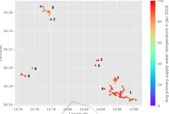
Figure 2 shows the groups and graph network rep-resentation produced by applying MST clustering on the above mentioned 70 substations. The substations are partitioned into nine clusters by applying the MST clustering algorithm while the cut-off parameter is set to 500 meters. That is substations with distance less
14.74
14.76
14.78
14.80
14.82
14.84
14.86
14.88
Longitude
56.16
56.18
56.20
56.22
56.24
56.26
Latitude
0
20
40
60
80
100
Avg primary supply water temperature in Jan 2018.
0 1 2 3 4 5 6 7 8
Figure 2: 70 substations located in Southern Sweden are grouped into nine clusters using the MST clustering algorithm. The geographical location of the substations is referred to as the Location view (v0). Substations with distance less than 500 meters
from their closest neighbours are grouped together. The color of the substations represents the average Ts,1stin January 2018,
which for most substations is around 87 °C.
than 500 meters from their closest neighbour(s) are grouped together. Five clusters represent as a tree, i.e., edges of the tree represent the distance between the substations (the tree nodes) and the remaining four clusters are singletons. The substations’ colors repre-sent their received average Ts,1st(°C) in January 2018. In order to make the data ready for the experi-ment, first the duplicates are removed. Then we fo-cused on extreme values which can appear as a result of faults in measurement tools. We apply a Hampel filter (Hampel, 1971) which is a median absolute de-viation (MAD) based estimation to detect and smooth out such extreme values. The filter is used with the default parameters, i.e., the size of the window is set to be seven and the threshold for extreme value detec-tion is set to be three.
In the studied context, we have hourly measure-ments data. This gives one time series every 24-hours and in total 365 time series per year. Time series with less than 24 measurement values are excluded. Since we are expecting different behaviours from a DH substation during heating and non-heating sea-sons, the time series are divided into two groups with respect to the outdoor temperature (To). That is, if
the outdoor temperature is above a certain threshold, Tothreshold, the DH substation behaviour can be cate-gorized into the non-heating season otherwise to the
heating season. This threshold in Sweden can be set to be Tothreshold= 10 °C. In order to assess each DH sub-station’s operational behaviours during heating sea-son and in comparisea-son with other substations, the ex-tracted time series are scaled with z-score normaliza-tion. That is, each time series is scaled to have a mean of zero and a standard deviation of one. Notice that in the considered context the general shape of the time series, rather than their amplitude, is important. Now for every category, the time series related to one spe-cific feature, i, can be compared in terms of similarity with respect to a distance measure d(yi, y0j), where d
in this study is DTW . This leads to a similarity ma-trix, SMi. In the next step, SMiis fed to a clustering
algorithm. Here we aim to group time series based on their similarities into a number of clusters. Con-sidering each feature as one view, we can analyse the operational behaviour of a set of DH substations by using the explained evaluation scenarios in Section 5.
6.2
Implementation and Availability
The proposed approach is implemented in Python ver-sion 3.6. The affinity propagation and the adjusted Rand index are adopted from the scikit-learn mod-ule (Pedregosa et al., 2011) and the MST clustering algorithm is fetched from (VanderPlas, 2016). The
alignments between time series are identified using dtwalign’s package2. The implemented code and the experimental results are available at GitHub3.
7
RESULTS AND DISCUSSION
The initial view in our analyses is always the outcome of the MST clustering, i.e., 70 substations in the stud-ied area are grouped into nine clusters based on their distances. We set the cut-off parameter to be 500 me-ters which means any edges greater than 500 meme-ters are removed from the MST. The first three clusters (0, 1, and 2) include 15, 32, and 14 substations, re-spectively (in total 61 of 70 substations). The remain-ing substations are grouped into 6 clusters as follows: cluster 3 contains 2 substations, clusters 4, 5, 7, and 8 are singletons and cluster 6 has 3 substations.
In the remainder of this study we only consider and discuss the results produced on clusters 0, 1, and 2, since the majority of the substations are distributed in these clusters. Each analysis can be performed based on different combinations of the features in Ta-ble 1. However, due to the page limit, we only report the results of the analyses with respect to Tr,1st and ∆T1st (the difference between Ts,1stand Tr,1st).
7.1
SW-MVC Analysis
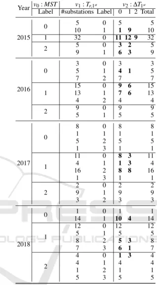
Table 2 shows the results of SW-MVC analysis for 61 substations throughout the heating seasons from 2015 to 2018. For each MST cluster (v0), initially
substations are grouped based on Tr,1st (v1) and then for each created subgroup the clustering analysis is performed using ∆T1st (v2). The information in Ta-ble 2 can be used in three different ways: column-wise, row-column-wise, or both. In the column-wise case, one can see how the substations in each MST cluster are grouped based on the other two views (i.e., v1and v2)
in different years. The row-wise analysis shows how the substations in each MST cluster are grouped step-wise based on first v1 and second v2. For example,
the domain experts might be interested in perform-ing further analysis when the grouped substations in v1are split into more subgroups based on v2.
Num-bers in bold in Table 2 represent the number of substa-tions that are grouped into different clusters based on v2as opposed to v1. By considering both cases one
can track the transition of the operational behaviour of substations throughout the years.
2https://github.com/statefb/dtwalign
3
https://github.com/shahrooz-abghari/MVC-DH-Monitoring
Table 2: SW-MVC analysis based on Tr,1st and ∆T1st from
2015 to 2018.
Year v0: MST v1: Tr,1st v2: ∆T1st Label #substations Label 0 1 2 Total
2015 0 5 0 5 5 10 1 1 9 10 1 32 0 11 12 9 32 2 5 0 3 2 5 9 1 6 3 9 2016 0 3 0 3 3 5 1 4 1 5 7 2 7 7 1 15 0 9 6 15 13 1 7 6 13 4 2 4 4 2 9 0 9 9 5 1 5 5 2017 0 8 0 8 8 1 1 1 1 5 2 5 5 1 3 1 1 1 11 0 8 3 11 4 1 1 3 4 16 2 8 8 16 1 3 1 1 2 2 0 2 2 9 1 9 9 3 2 3 3 2018 0 1 0 1 1 14 1 10 4 14 1 12 0 12 12 5 1 5 5 8 2 5 3 8 7 3 6 1 7 2 4 0 1 3 4 4 1 4 4 1 2 1 1 5 3 5 5
Note. Number of substations that are grouped into different clusters based on v2 as opposed to v1 are
shown inbold.
Figure 3 depicts the SW-MVC analysis by consid-ering Tr,1st as the first view (squares) and ∆T1st as the second view (circles) in the period from 2015 to 2018. Figure 4 represents the SW-MVC analysis specifi-cally for the MST cluster with label 0 during a period covering 2017 and 2018. Notice, the color of squares shows Tr,1st while the colored circles represent ∆T1st. These two features can be used as an assessment indi-cator for the operational behaviour of the substations. Technically, it is desired in a well performed substa-tion that the Tr,1st has a lower value in comparison to the Ts,1st. In other words, a greater delta means that the substation is making more efficient use of the sup-plied heat for space heating.
14.75 14.80 14.85 56.16 56.18 56.20 56.22 56.24 56.26
Latitude
2015
14.75 14.80 14.85 56.16 56.18 56.20 56.22 56.24 56.262016
14.75 14.80 14.85Longitude
56.16 56.18 56.20 56.22 56.24 56.26Latitude
2017
14.75 14.80 14.85Longitude
56.16 56.18 56.20 56.22 56.24 56.262018
39 40 41 42 43 44Temperature °C
41 42 43 44 45 46Temperature °C
38 40 42 44 46 48Temperature °C
40 41 42 43 44 45Temperature °C
Figure 3: The results of SW-MVC analysis for the whole studied area contains 70 substations. Squares represent clusters of substations based on the first view, Tr,1st, and circles represent groups of substations with respect to the second view, ∆T1st.
Note that the substations with similar colors in different MST clusters are not related.
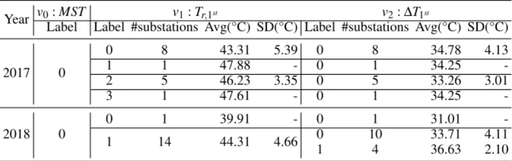
of the actual measurements and their standard devia-tions, regarding the DH substations that are discussed in Figure 4. As one can see in 2017, substations are grouped into 4 clusters, where clusters 0 (green squares) and 2 (orange squares) contains the major-ity of substations, 8 and 5, respectively. The two other clusters include only one substation each (red squares). The average Tr,1st for cluster 0 is approxi-mately 43 °C and for cluster 2 is around 46 °C. Clus-ters 1 and 3 both show the average Tr,1st of 48 °C. All the grouped substations in the previous step stayed to-gether based on the ∆T1st, i.e., no new cluster is cre-ated. The cluster with 8 substations (grey circles in-side green squares) represents the ∆T1st of 34.79 °C, while the cluster with 5 substations (yellow circles in-side orange squares) shows the ∆T1stof 33.26 °C. The other two clusters (yellow circles inside red squares) show the same value, 34.25 °C for the ∆T1st.
In 2018, the same number of substations, 15, are grouped into only two clusters with an average Tr,1st of approximately 40 °C for cluster 0 (purple square) and 44 °C for cluster 1 (orange squares). A majority of the substations, 13 out of 14, are grouped in clus-ter 1. This clusclus-ter is further divided into two clusclus-ters, one with 10 DH substations (grey circles inside or-ange squares) and the average ∆T1st of approximately 34 °C and the other with 4 substations (orange cir-cles inside orange squares) and the average ∆T1st of
14.77
14.78
Longitude
56.258
56.260
56.262
56.264
56.266
56.268
Latitude
2017
33.26°C
34.25°C
34.78°C
14.77
14.78
Longitude
56.258
56.260
56.262
56.264
56.266
56.268
Latitude
2018
31.01°C
33.71°C
36.63°C
38
40
42
44
46
48
Temperature °C
40
41
42
43
44
45
Temperature °C
Figure 4: The results of SW-MVC analysis for the MST cluster with label 0 and 15 substations in 2017 (top) and 2018 (bottom). Colored squares represent groups of substa-tions based on v1: Tr,1stand colored circles represent groups
Table 3: SW-MVC analysis for the MST cluster with label 0, 2017 to 2018.
Year v0: MST v1: Tr,1st v2: ∆T1st
Label Label #substations Avg(°C) SD(°C) Label #substations Avg(°C) SD(°C)
2017 0 0 8 43.31 5.39 0 8 34.78 4.13 1 1 47.88 - 0 1 34.25 -2 5 46.23 3.35 0 5 33.26 3.01 3 1 47.61 - 0 1 34.25 -2018 0 0 1 39.91 - 0 1 31.01 -1 14 44.31 4.66 0 10 33.71 4.11 1 4 36.63 2.10
Note. Avg: average, SD: standard deviation
approximately 37 °C. Cluster 0 represents one sub-station (yellow circle inside purple square) with the average ∆T1stof 31.01 °C. In both years there are sub-stations that show slightly different operational be-haviour in comparison to their neighbouring substa-tions, e.g., the red substations in 2017 and the purple substation in 2018. The domain experts can investi-gate the reasons why these substations performed dif-ferently in comparison to the majority of substations. In addition, it is important to mention that the order in which views are used for the SW-MVC analysis af-fects the results, which can be decided based on the domain expert’s preferences.
7.2
PW-MVC Analysis
The aim of this analysis is to group the substations based on two different views (i.e., v1and v2) and
com-pare the results of the clustering solution to find out which substations are similar based on both views. Such analysis can provide useful information for the domain experts while it applies for a period of time, e.g., different years, where the transition of the opera-tional behaviour of substations can be monitored. Ta-ble 4 shows the distribution of the studied substations based on PW-MVC analysis throughout the heating season in the period from 2015 to 2018.
Figure 5 depicts the computed ARI scores for the clustering solution based on Tr,1st and ∆T1st of each MST cluster in the period from 2015 to 2018. As one can see, the ARI scores of the first three clus-ters are absolutely dissimilar in 2015, 2016, and 2018. However, cluster 2 with 14 substations shows the ARI score of 0.71 in 2017, which means the majority of DH substations in this cluster performed similarly. Other clusters, 3 to 8 represent the adjusted Rand in-dex of 1 for all the years.
Figure 6 shows the PW-MVC analysis for MST cluster with label 1 with respect to Tr,1st and ∆T1st in the period from 2015 to 2018. The substations with similar cluster labels with regard to both features are shown in red. The insight provided by Figure 6 can
Table 4: PW-MVC analysis is performed based on Tr,1stand
∆T1st separately from 2015 to 2018. Year v0: MST v1: Tr,1st v2: ∆T1st Label #substation 0 1 2 3 0 1 2 2015 0 15 5 10 5 10 1 32 32 11 12 9 2 14 5 9 6 5 3 Total 70 51 19 31 27 12 2016 0 15 3 5 7 6 9 1 32 15 13 4 32 2 14 9 5 10 4 Total 70 36 23 11 57 13 2017 0 15 8 1 5 1 15 1 32 11 4 16 1 10 22 2 14 2 9 3 10 4 Total 70 30 14 24 2 44 26 2018 0 15 1 14 9 6 1 32 12 5 8 7 26 6 2 14 4 4 1 5 4 10 Total 70 26 23 9 12 48 22 (0, 15) (1, 32) (2, 14) (3, 2) (4, 1) (5, 1) (6, 3) (7, 1) (8, 1)
(MST label, No. substations)
0.0 0.2 0.4 0.6 0.8 1.0
Adjusted Rand Index
2015 2016 2017 2018
Figure 5: PW-MVC analysis, the computed ARI scores for Tr,1stand ∆T1stthroughout 2015 to 2018.
be used for analysing the difference between oper-ational behaviour of the red substations against the greys within one specific year. In addition, the transi-tion of the substatransi-tions from one color group to another can be tracked and further analysed.
14.85
14.86
14.87
14.88
14.89
56.165
56.170
56.175
56.180
Latitude
2015
14.85
14.86
14.87
14.88
14.89
56.165
56.170
56.175
56.180
2016
14.85
14.86
14.87
14.88
14.89
Longitude
56.165
56.170
56.175
56.180
Latitude
2017
14.85
14.86
14.87
14.88
14.89
Longitude
56.165
56.170
56.175
56.180
2018
Figure 6: The results of PW-MVC analysis for the MST cluster with label 1 and 32 substations. Substations in red are those that are grouped with the same label according to the both views, namely Tr,1stand ∆T1stfrom 2015 to 2018.
8
CONCLUSIONS
We have proposed a multi-view clustering approach for analysing datasets that consist of different data representations. The proposed approach has been ap-plied for monitoring and analysing operational be-haviour of district heating substations. We have ini-tially used the substations’ geographical information to build an approximate graph representation of the DH network. This graph structure has been used as a backbone for further analysis of the network perfor-mance.
In the above context, we have proposed and dis-cussed two different types of analysis: 1) step-wise multi-view clustering that sequentially considers and analyses the operational behaviour of the DH substa-tions with respect to different views and organizes the substations into a hierarchical structure. That is, at each step a new clustering solution is built on top of the one generated in the previous step with respect to the considered view. 2) parallel-wise multi-view clus-tering that analyses substations with regards to two different views in side by side. This enables the iden-tification of the relationships between neighbouring
substations by organizing them in a bipartite graph and analysing their distribution with respect to the two considered views. The proposed data analysis ap-proach facilitates the visual analysis and inspections of multi-view real-world datasets such as ones related to the DH networks. For example, the proposed ap-proach provides the opportunity to consider the DH substations in close relation with their neighbours. That is, those substations that demonstrate a deviat-ing behavior from their neighbourdeviat-ing substations can easily be identified for further investigation.
For future work, we are interested in expanding our approach by adding a third scenario where the clustering solution is the outcome of integration of different views. We believe that the proposed ap-proach provides a verity of analysis techniques to sup-ply the domain experts with a complete picture about the DH network operations. In addition, the proposed approach can facilitate the identification of substa-tions with deviating behaviours and suggest initiation of further inspections by domain experts.
ACKNOWLEDGEMENTS
This work is part of the research project “Scal-able resource-efficient systems for big data analyt-ics“ funded by the Knowledge Foundation (grant: 20140032) in Sweden.
We would also like to thank Christian Johansson, CEO of NODA Intelligent Systems, for his support and valuable feedback.
REFERENCES
Abghari, S., Boeva, V., Brage, J., Johansson, C., Grahn, H., and Lavesson, N. (2019). Higher order mining for monitoring district heating substations. In 2019 IEEE Int’l Conf. on Data Science and Advanced Analytics (DSAA), pages 382–391. IEEE.
Ando, R. K. and Zhang, T. (2007). Two-view feature gener-ation model for semi-supervised learning. In Proc. of the 24th Int’l Conf. on Machine learning, pages 25– 32. ACM.
Bickel, S. and Scheffer, T. (2004). Multi-view clustering. In ICDM, volume 4, pages 19–26.
Blum, A. and Mitchell, T. (1998). Combining labeled and unlabeled data with co-training. In Proc. of the eleventh annual Conf. on Computational learning the-ory, pages 92–100.
Cai, X., Nie, F., and Huang, H. (2013). Multi-view k-means clustering on big data. In Twenty-Third Int’l Joint Conf. on artificial intelligence.
Calikus, E., Nowaczyk, S., Sant’Anna, A., Gadd, H., and Werner, S. (2019). A data-driven approach for dis-covery of heat load patterns in district heating. arXiv preprint arXiv:1901.04863.
Deepak, P. and Anna, J.-L. (2019). Multi-View Clustering, pages 27–53. Springer Int’l Publishing, Cham. Frederiksen, S. and Werner, S. (2013). District Heating and
Cooling. Studentlitteratur AB.
Frey, B. J. and Dueck, D. (2007). Clustering by passing messages between data points. Science, 315(5814):972–976.
Hampel, F. R. (1971). A general qualitative definition of robustness. The Annals of Mathematical Statistics, pages 1887–1896.
Hubert, L. and Arabie, P. (1985). Comparing partitions. J. of classification, 2(1):193–218.
Isermann, R. (1997). Supervision, detection and fault-diagnosis methods—an introduction. Control engi-neering practice, 5(5):639–652.
Isermann, R. (2006). Fault-diagnosis systems: an introduc-tion from fault detecintroduc-tion to fault tolerance. Springer Science & Business Media.
Jiang, B., Qiu, F., and Wang, L. (2016). Multi-view cluster-ing via simultaneous weightcluster-ing on views and features. Applied Soft Computing, 47:304–315.
Katipamula, S. and Brambley, M. R. (2005a). Methods for fault detection, diagnostics, and prognostics for
building systems-A review, part I. Hvac&R Research, 11(1):3–25.
Katipamula, S. and Brambley, M. R. (2005b). Methods for fault detection, diagnostics, and prognostics for build-ing systems-A review, part II. Hvac&R Research, 11(2):169–187.
Kumar, A. and Daum´e, H. (2011). A co-training approach for multi-view spectral clustering. In Proc. of the 28th Int’l Conf. on machine learning (ICML-11), pages 393–400.
Liu, J., Wang, C., Gao, J., and Han, J. (2013). Multi-view clustering via joint nonnegative matrix factorization. In Proc. of the 2013 SIAM Int’l Conf. on Data Mining, pages 252–260. SIAM.
MacQueen, J. et al. (1967). Some methods for classification and analysis of multivariate observations. In Proc. of the Fifth Berkeley Symp. on Mathematical Statistics and Probability, volume 1, pages 281–297. Oakland, CA, USA.
Meng, X., Liu, X., Tong, Y., Gl¨anzel, W., and Tan, S. (2015). Multi-view clustering with exemplars for sci-entific mapping. Scientometrics, 105(3):1527–1552. Pedregosa, F., Varoquaux, G., Gramfort, A., Michel, V.,
Thirion, B., Grisel, O., Blondel, M., Prettenhofer, P., Weiss, R., Dubourg, V., Vanderplas, J., Passos, A., Cournapeau, D., Brucher, M., Perrot, M., and Duch-esnay, E. (2011). Scikit-learn: Machine learning in Python. J. of Machine Learning Research, 12:2825– 2830.
Rand, W. M. (1971). Objective criteria for the evaluation of clustering methods. J. of the American Statistical association, 66(336):846–850.
Sakoe, H. and Chiba, S. (1978). Dynamic programming algorithm optimization for spoken word recognition. IEEE Transactions on Acoustics, Speech, and Signal Processing, 26(1):43–49.
Sandin, F., Gustafsson, J., and Delsing, J. (2013). Fault de-tection with hourly district energy data: Probabilistic methods and heuristics for automated detection and ranking of anomalies. Svensk Fj¨arrv¨arme.
VanderPlas, J. (2016). mst clustering: Clustering via eu-clidean minimum spanning trees. J. Open Source Soft-ware, 1(1):12.
Wang, C.-D., Lai, J.-H., and Philip, S. Y. (2015). Multi-view clustering based on belief propagation. IEEE Transactions on Knowledge and Data Engineering, 28(4):1007–1021.
Wang, X., Qian, B., Ye, J., and Davidson, I. (2013). Multi-objective multi-view spectral clustering via pareto op-timization. In Proc. of the 2013 SIAM Int’l Conf. on Data Mining, pages 234–242. SIAM.
Xu, C., Tao, D., and Xu, C. (2013). A survey on multi-view learning. arXiv preprint arXiv:1304.5634.
Xue, P., Zhou, Z., Fang, X., Chen, X., Liu, L., Liu, Y., and Liu, J. (2017). Fault detection and operation optimiza-tion in district heating substaoptimiza-tions based on data min-ing techniques. Applied Energy, 205:926–940. Zong, L., Zhang, X., Zhao, L., Yu, H., and Zhao, Q. (2017).
Multi-view clustering via multi-manifold regularized non-negative matrix factorization. Neural Networks, 88:74–89.