Effluents quality prediction by using nonlinear dynamic block-oriented models: A system identification approach

* Corresponding author.

1944-3994/1944-3986 © 2021 Desalination Publications. All rights reserved.

www.deswater.com

doi: 10.5004/dwt.2021.26983

Effluents quality prediction by using nonlinear dynamic block-oriented

models: a system identification approach

S.I. Abba

_{*, R.A. Abdulkadir}

_{, M.S. Gaya}

_{, Saad Sh. Sammen}

_{, Umar Ghali}

_,

M.B. Nawaila

_{, Gözde Oğuz}

_{, Anurag Malik}

_{, Nadhir Al-Ansari}

a_{Department of Physical Planning Development, Yusuf Maitama Sule University, Kano 700221, Nigeria, email: saniisaabba86@gmail.com} b_{Department of Electrical Engineering, Kano University of Science & Technology, Wudil, Nigeria, emails: rabiukk@gmail.com}

(R.A. Abdulkadir), muhdgayasani@gmail.com (M.S. Gaya)

c_{Department of Civil Engineering, College of Engineering, University of Diyala, Diyala Governorate, Iraq, email: Saad123engineer@yahoo.com} d_{Department of Medical Biochemistry, Faculty of Medicine, Near East University, 99138 Nicosia, North Cyprus, Mersin-10,}

Turkey, email: umarghali18@gmail.com

e_{Department of Computer Science Education, Aminu Saleh College of Education, Azare, Nigeria}

f_{Faculty of Civil and Environmental Engineering, Near East University 99138 Nicosia, North Cyprus, Mersin 10, Turkey,}

email: gozde.oguz@neu.edu.tr

g_{Department of Electrical and Electronic Engineering, Near East University, Nicosia - North Cyprus, via Mersin 10, Turkey}

h_{Punjab Agricultural University, Regional Research Station, Bathinda-151001, Punjab, India, email: anuragmalik_swce2014@rediffmail.com} i_{Civil, Environmental and Natural Resources Engineering, Lulea University of Technology, 97187 Lulea, Sweden,}

email: nadhir.alansari@ltu.se

Received 16 June 2020; Accepted 21 December 2020

a b s t r a c t

The dynamic and complex municipal wastewater treatment plant (MWWTP) process should be handled efficiently to safeguard the excellent quality of effluents characteristics. Most of the avail-able mathematical models do not efficiently capture the MWWTP process, in such cases, the data-driven models are reliable and indispensable for effective modeling of effluents characteristics. In the present research, two nonlinear system identification (NSI) models namely; Hammerstein-Wiener model (HW) and nonlinear autoregressive with exogenous (NARX) neural network model, and a classical autoregressive (AR) model were proposed to predict the characteristics of the effluent of total suspended solids (TSS_eff) and pH_eff from Nicosia MWWTP in Cyprus. In order to attain the optimal models, two different combinations of input variables were cast through auto-correla-tion funcauto-correla-tion and partial auto-correlaauto-correla-tion analysis. The predicauto-correla-tion accuracy was evaluated using three statistical indicators the determination coefficient (DC), root mean square error (RMSE) and correlation coefficient (CC). The results of the appraisal indicated that the HW model outperformed NARX and AR models in predicting the pH_eff, while the NARX model performed better than the HW and AR models for TSSeff prediction. It was evident that the accuracy of the HW increased averagely up to 18% with regards to the NARX model for pH_eff. Likewise, the TSS_eff performance increased averagely up to 25% with regards to the HW model. Also, in the validation phase, the HW model yielded DC, RMSE, and CC of 0.7355, 0.1071, and 0.8578 for pH_eff, while the NARX model yielded 0.9804, 0.0049 and 0.9902 for TSS_eff, respectively. For comparison with the traditional AR, the results showed that both HW and NARX models outperformed in (TSS_eff) and pH_eff prediction at the study location. Hence, the outcomes determined that the NSI model (i.e., HW and NARX) are reliable and resilient modeling tools that could be adopted for pH_eff and TSS_eff prediction.

Keywords: Municipal wastewater; Hammerstein-Wiener model; Nonlinear autoregressive with

1. Introduction

Municipal wastewater management is necessary to protect our environment from deterioration – as well as to improve the water scarcity, which exists in a place where the water is insufficient to meet satisfy requirements demands [1]. A municipal wastewater treatment plant (MWWTP) is an extremely complex and dynamic process due to its intricacy of the treatment method. Appropriate action, maintenance, and control of MWWTPs are very vital for monitoring envi-ronmental and ecological health [2]. The total suspended solids (TSS) and pH are some of the most significant vari-ables that govern the efficiency of the effluent characteris-tics in any treatment plant. Control of pH by the addition of some basic chemicals (acidic and base) is an integral part of any sewage treatment system as it permits dissolved to be separated during the entire treatment process [3,4]. Generally, a pH value beyond the prescribed standard (6–9) can significantly disturb the ongoing process of bac-teria and other microorganisms. Hence, it is obvious that there is a need to employed and an efficient model that can precisely estimate the pH concentration in the system [5].

Due to the importance of management, planning, and control of wastewater, the modeling approach in this field remains dynamic and active of study. Physical-based and data-driven models are the two mains categories applied to hydro-environmental studies. The concept of distributed white box is applied to physical models to address inter-action for simulating the hydro-environmental system and the physical processes. While optimal links between out-put and inout-put are acquired on a lumped (black box) model that is based on data-driven, in which the physical process is neglected [6,7]. Various efforts have been presented to improve the accuracy and reliability of the effluent vari-ables in the field of hydro-environmental studies. Still, no individual method has been proved applicable in modeling environmental processes [8,9]. With regards to this perspec-tive, there is a necessity to develop a reliable and efficient model that can deal with the dynamics and complexity of data of hydro-environmental systems, because, no single model proves to be acceptable as the best based on best performance [10–13].

Besides, the process of MWWTP has both deterministic and stochastic systems. A stochastic model such as autore-gressive (AR) has been used in modeling and prediction of hydrological process, especially time-series process [6]. The AR model is widely known for moderation and sim-plicity among the linear models and is employed in several modeling studies [14,15]. Owing to its linear nature, AR may not reliably and properly model the possibly intricate processes taking place in MWWTP [16].

Based on the established wastewater treatment plant studies (WWTP), linear and conventional regression tools have been widely used but they have been generally asso-ciated with low accuracy levels, giving room to the devel-opment of the artificial intelligence (AI) methods which are considered as accurate and nonlinear modeling tools [17–19]. Meanwhile, several researchers have established different types of AI techniques which have been gradually applied for modeling and estimation in various discipline of hydrology and environmental engineering to rescue the

existing traditional models [7,20–23]. For example, Memon et al. [4] developed an artificial neural network (ANN) with a multi-layer perceptron (MLP) model to forecast the treated and untreated pH using 17 measured input parameters in the water treatment plant (WTP), Hyderabad (Pakistan). The outcomes proved the suitability of MLP in modeling the drinking WTP parameters. Verma and Singh [24] stud-ied the potential of five different data mining approaches includes MLP, support vector machine (SVM), regression forest (RF), k-nearest neighbors (KNN), and multivari-ate adaptive regression spline (MARS) to predict daily TSS from WWTP located in Des Moines, Iowa. The result showed that the MLP model achieved the best prediction and therefore outperformed all other models.

Similarly, Granata et al. [25] attempted to simulate wastewater quality indicators such as biological oxygen demand, chemical oxygen demand (COD), total dissolved solids (TDS) and TSS using numerous types of machine learning algorithms such as support vector regression (SVR) and regression tree (RT). From the outcomes, it was observed that both models showed robustness and reliabil-ity in the prediction. However, a significant performance of SVR was observed compared with RT in modeling the effluent TDS, TSS, and COD. Gaya et al. [26] applied the ANN and Hammerstein-Wiener (HW) models for forecast-ing the influent turbidity in Tamburawa WTP usforecast-ing differ-ent input parameters. The results indicated that ANN out-performs the HW model and could serve as an acceptable tool for modeling the turbidity of WTP.

However, the results of prediction produced by some of these models still suffered from various imprecision and inadequacies despite the growing application and useful-ness of the AI model. Therefore, it has become necessary to design a universally applicable and robotic AI model that can be applied in diverse fields. The novelty of this study is using nonlinear system identification (NSI) mod-els to predict the characteristics of the effluents. Hence, Nicosia MWWTP is considered as a case study in order to implement the ability of data-intelligence approaches such as AR and NSI models (i.e., HW and NARX – nonlinear autoregressive with exogenous) to predict the TSS and pH effluents (TSS_eff and pH_eff). For this purpose, the modeling performance of HW, NARX and AR models was evaluated using efficiency indicators and graphical inspection. 2. Material and methods

2.1. Nicosia municipal wastewater treatment plant and data collection

It was reported that management, control and planning of wastewater exist to be the highest tool for bi-commu-nal collaboration among the two peoples of Nicosia since the 1960s. The new Nicosia MWWTP is a bi-communal project serving two different communities between Turkish Cypriot and Greek Cypriot. The project was jointly founded by the sewage board of Nicosia and the European Union (EU) and implemented by United Nations Development Programme (UNDP). For sustainable development and recycling purposes, more than 300 tons/y will be generated. A total of about 10 million m³ of quality effluent can be reused

for different agricultural purposes [27,28]. The essential components of Nicosia MWWTP are demonstrated in Fig. 1.

The daily measured data obtained from new Nicosia MWWTP which includes (pH_inf, COD_inf, Total-N_inf, NH₄– N_inf, SS_inf, and TSS_inf) as the input variables and (pH_eff, TSS_eff) as the corresponding output of the model. The normal-ized data were divided into 75% and 25% for both calibra-tion and validacalibra-tion, respectively, between 2015 and 2016. The validation methods are implemented using different approaches; this study employed a holdout approach which is known as leave-group-out. In this approach, the data randomly assigned to two sets generally named calibra-tion and validacalibra-tion and can be regarded as another version of k-fold cross-validation [29–31].

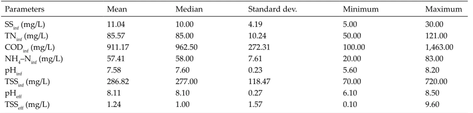
The concentration of the treated pH and TSS (mg/L) at the exit before the discharge to the receiving body is shown in Fig. 2. It can be seen from the figure that the time-series and box-whiskers plots indicate the profile, range, and the extents of outliers in each parameter. The range indicated that both pH and TSS values are within the prescribed efflu-ent standards by Environmefflu-ental Protection Agency (EPA) (pH = 5–9 and TSS = 35 mg/L). Some of the measured daily data were outliers, especially for TSS_eff. This explains the discrepancy between the numbers of samples even though the distribution of outliers is not far away from normality as in the case of TSS_eff. Despite some fitting methods may be applied to overcome the problems of outliers and also fill the missing data before modeling but in this case, the data may be appropriate for modeling since it contained fewer outli-ers that can be taking care by NSI models and the deviation of outliers from the average is insignificant. Table 1 gives a summary of the basic descriptive statistics of the data.

2.2. Autoregressive model

The degree of uncertainty and randomness that builds the stochastic process of an AR model makes it commonly used in time series simulations [6,32,33]. Base on the prior

variables value knowledge, the AR model forecasts the value of the future. Therefore, the AR model for an order

p is defined as AR(p) and expressed as:

Xt=β1Xt−1+β2Xt−2+ …∈t (1)

(b)

Fig. 2. (a) Effluent pH and (b) TSS concentration at Nicosia MWWTP.

where ∈_t is white noise with E = (∈_t) and VAR(∈_t) = σ_e2_,

the parameters β₁, β₂, …, β_P are AR coefficients (Hadi and Tombul [6]).

2.3. Hammerstein-Wiener model

Hammerstein-Wiener is a model that follows and pre-cedes a linear dynamic even though it’s a nonlinear block (Fig. 3) [26,33–36]. For the identification of a nonlinear sys-tem, a black box model as HW was developed [37]. The combination of parallel and series interconnected non-linear dynamics and static blocks made up HW as shown in Fig. 3 [36]. An appropriate illustration of the HW was characterized by an understandable and clear relationship between nonlinear and linear systems than the other tra-ditional ANN. The HW finds and captures simple para-metric functionality about the system characteristics and specifications for nonlinear models [33].

Fig. 3 depicts w(t) = f(u(t)) is a nonlinear function con-verting input data, x(t) = w(t)B/F shows linear transfer function, f and h act on the input and output part of the linear block, respectively, the function w(t) and x(t) are variables that define the input and output of the linear block.

2.4. Nonlinear autoregressive with exogenous neural network

The NARX neural network (NN) is a nonlinear recur-rent dynamic neural network, implemented with feedback connections and consisting of several layers [37]. This NARX model is based on the linear autoregressive with exogenous (ARX) model, which is frequently used in time series modeling. Therefore, NARX can accept dynamic inputs represented by time series sets. This represents the main advantage of the NARX NN over feedforward back-propagation neural networks [38,39]. As recurrent neural

network possesses the network are quite suitable for nonlin-ear function approximation and control. The configuration of the NARX model in both series and parallel can be shown in Fig. 4. The expression for the NARX model is given as:

y t

( )

(

( )

(

)

(

)

( )

(

)

(

)

)

n_u are the maximum lags input and output entering the model, respectively. The predicted output of future value

y k +p

(

)

y kp y kp y kp y k np u k u k n

 +

₍

₎

( )

( )

(

) ( )

(

)

2.5. Model development and performance indicators

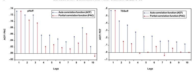
For the development of the model, the obtained data from the new Nicosia MWWTP were divided into 75% for calibration and 25% for validation with a total of 360 instances. Different methods were reported for input selec-tion, such as (i) Pearson and Spearman correlation analysis to determine the strength and relations between inputs and outputs (Table 2) and (ii) auto-correlation function (ACF) and the partial auto-correlation (PAC) [40,41]. Subsequently, a set of two different models were derived based on significant input variables presented in Table 3.

For any time-series modeling identifying the proper time lags is a very essential part of selecting the appropriate Table 1

Daily values of basic descriptive statistical indices for used data

Parameters Mean Median Standard dev. Minimum Maximum

SS_inf (mg/L) 11.04 10.00 4.19 5.00 30.00 TN_inf (mg/L) 85.57 85.00 10.24 50.00 121.00 COD_inf (mg/L) 911.17 962.50 272.31 100.00 1,463.00 NH₄–N_inf (mg/L) 57.41 58.00 7.61 20.00 83.00 pH_inf 7.58 7.60 0.23 5.60 8.20 TSS_inf (mg/L) 286.82 277.00 118.47 70.00 720.00 pH_eff 8.11 8.10 0.27 6.10 8.50 TSS_eff (mg/L) 1.24 1.00 1.57 0.10 9.60

model inputs combinations, as such ACF and PAC are used (Fig. 5). The correlation between forthcoming and previ-ous data points is considered as a time series correlation. For instance, for a time X, the correlation (R) of the first lag (lag 1) is considered as the R between X_t and X_t–1; for the second lag (lag 2) is considered as R between X_t and X_t–2. On the other hand, the partial correlation is the R-value of a parameter with its lag that is yet to be described by the

R of the lower lags [6]. Data normalization is often used

as a pre-processing stage prior to the model calibration to improve the accuracy and speed of the models [12,18]. For this work, the normalization is implemented using Eq. (4). Machine learning models and mathematical models are evaluated using numerical indicators. The NSI models developed in this study were inspected using three statis-tical metrics, including determination coefficient (DC), root mean square error (RMSE), and correlation coefficient (CC) (Eqs. (5)–(7)).

Spearman and Pearson’s correlation describes how well the relationship between the variables can be described

using a linear and monotonic function. The strength of the correlation is not dependent on the direction or sign. A positive coefficient indicates that an increase in the first parameter would correspond to an increase in the sec-ond parameter while the negative correlation indicates an inverse relationship whereas one parameter increases and the second parameter decreases [42,43]. It can be seen from Table 2 that, after performing correlation analysis (R) for selecting the initial input variables, a significant R was observed between the variables.

y x x x x = + × − −             0 05. 0 95. min max min (4) where y is the normalized data, x is the measured data,

x_max and x_min are the maximum and minimum values of the measured data, respectively. The prediction accuracy of developed models was assessed by using NSE, RMSE, and CC [44].

Fig. 4. Architectures of the NARX neural network (Men et al., 2014).

AQ6

Table 2

Pearson and Spearman correlation analysis of the parameters

Parameters pH_inf COD_inf TN_inf NH₄–N_inf SS_inf TSS_inf pH_eff TSS_eff

pH_inf 1 CODinf –0.1599 1 TN_inf 0.0527 0.1353 1 NH₄–N_inf 0.2512 0.1009 0.5037 1 SSinf –0.0051 0.1015 0.3346 0.0919 1 TSS_inf 0.0098 0.1726 0.1547 0.0409 0.4852 1 pH_eff 0.0252 0.3564 0.1387 0.1475 0.4021 0.0766 1 TSSeff 0.1426 –0.5836 –0.5909 0.0665 –0.6743 0.0800 0.0556 1 Table 3

Developed models with input–output variables

Model output Model Input variables

Effluent pH (pH_eff) M1 (4) SSinf + TNinf + CODinf + NH4–Ninf

M2 (6) SS_inf + TN_inf + COD_inf + NH₄–N_inf + pH_inf + TSS_inf Effluent TSS (TSS_eff) M1 (4) SSinf + TNinf + CODinf + NH4–Ninf

DC obs obs pre pre

obs obs pre

= −

(

)

(

)

(

)

∑

∑

(

)

(

)

∑

RMSE= obs pre RMSE

−

(

)

(

)

∑

CC obs obs pre pre

obs obs pre pr

=

(

)

(

)

(

)

∑

(

)

(

)

∑

∑

where N, Y_obs,i, Y_pre,i, Y_obs and Y_pre are data number, observed and predicted data, an average value of the observed and computed data for ith values, respectively.

3. Results and discussion

The HW and NARX models were developed using MATLAB2019a system identification toolbox in such a way that the output and the input nonlinearity configura-tion on the model have several units equal to 10 as default and prewire linear function, the complexity of the model increases proportionally with the number of units for HW model. Similarly, for the NARX model, specify delay and number of terms in neural network regressor are chosen according to the input variables. The augmented Dickey–Full stationary test was conducted to meet the normality assumption of the AR model [45]. Fig. 5 shows the variation of ACF and PAC values. It was noticed from Fig. 5 that the maximum number of lags (10) employed in the first analysis. Both the ACF and PAC are obtained to identify the number of the lags to be considered, the order of the AR lags was identified by using PAC. For this research. The PAC for pH_eff and TSS_eff was considered as 4 and 6 lags, and this is because the first 4 lags have the

highest ACF followed by the next two lags. Therefore, the lags considered (4 and 6) is equal to the number of devel-oped models for each target outcome. For all the models, M1 (4) represents the model with four input combinations while in the case of AR, it indicates the model with four lags.

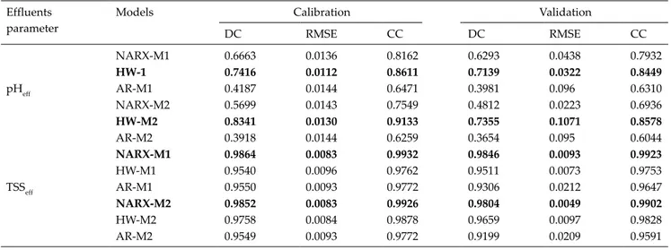
Table 4, displays the direct evaluation and compar-ison between the two models, it can be observed that HW and NARX model attained the highest accuracy in terms of performance indicators for the estimation of pH_eff and TSS_eff, respectively. Among the model combina-tion, M2 (6) outperformed M1 (4) in pH_eff estimation with approximately 9% and 2% for both calibration and vali-dation, respectively. On the other hand, M1 (4) emerged to be the best model for the estimation of TSS_eff with an average of 4% in both calibration and validation periods. The optimal AR model for both the pH_eff and TSS_eff was AR M1 (4) consisting of 4 inputs variables and lag days (Table 3). In general, NSI models are found to be close to each other and the results are better than the linear AR model.

Some graphical presentations were also used to exam-ine the performance of the HW, NARX and AR models, such as time series, radar chart, and Taylor diagrams. Figs. 6 and 7 illustrate the time series plots of the observed vs. the computed pH_eff and TSS_eff for the applied models in the validation phase. It is clear from Fig. 6 that HW-M1 and M2 have determination coefficient (DC) = 0.7416 and 0.8341 for calibration, DC = 0.7139 and 0.7355 for validation in pH_eff prediction, while Fig. 7 shows the NARX-M1 and M2 have DC = 0.9864 and 0.9852 for calibration, DC = 0.9846 and 0.0.9804 for validation in TSS_eff prediction. It is clear also from Figs. 6 and 7 that the fitted values of all three mod-els proved the superiority of 4 lags/input combinations (i.e., SS_inf + TN_inf + COD_inf + NH₄–N_inf) over six lags/input com-binations (i.e., SS_inf + TN_inf + COD_inf + NH₄–N_inf + pH_inf + TSS_inf). A further method for diagnostic analysis of the models was employed using the Taylor diagram [46], which can highlight the performance efficiency and accuracy of mod-els based on the observed values. The visual judgment of the model performance is provided by a polar plot using the Taylor diagram and shows three different (i.e., correla-tion coefficient, normalized standard deviacorrela-tion, and RMSE). Figs. 8a and b provide the Taylor diagrams for pH_eff and

-.1 .0 .1 .2 .3 .4 .5 .6 1 2 3 4 5 6 7 8 9 10 Auto correlation function (ACF) Partial correlation function (PAC)

Lags AC F/ PC F TSSeff -.02 .00 .02 .04 .06 .08 .10 .12 .14 1 2 3 4 5 6 7 8 9 10 Auto correlation function (ACF) Partial correlation function (PAC) pHeff Lags AC F/ PA C

TSS_eff, respectively for the validation period. Taylor’s dia-gram also confirmed the superiority of the HW model in pH_eff and NARX model in TSS_eff prediction in comparison to the AR model.

Furthermore, the prediction accuracy of HW (M1 and M2) NARX (M1 and M2) and AR (M1 and M2) mod-els for pH_eff and TSS_eff, are illustrated through radar-chart in Figs. 9a and b, respectively. These plots strengthened the justification performance evaluations mentioned in Table 4. Figs. 9a and b demonstrate the radar chart shows the different varieties of CC in both calibration and valida-tion. From these figures, it can be seen that the 0.6044 and 0.9902 are the lowest and highest value of CC obtained from all the models in the validation phase. As it was reported in several research that the high-value of CC attributes in providing the best performing model [34].

The exploratory analysis for HW NARX and AR mod-els can also be justified and better visualized through box-plots (Fig. 10). A powerful graphical Boxplot overview of data representation gives the summary of the data set, based on the mean value, the closest to the all observed val-ues to the models are given according to Fig. 10, the plot contained (box and whisker median, mean and staples). According to the plot, the extent of spread values between the predicted and observed models indicates that the pH_eff (HW-2) and TSS_eff (NARX-M1) ranked the best model.

To concur the finding of the current research were com-pared with the several existed studies on multiple param-eter prediction of wastewater treatment plant (WWTP) by employing numerous data-driven models [24,35,47,48] examined the comparative potential of MLP, KNN, MARS, SVM, and RF for predicting the TSS from WWTP set in Des

0.0 0.2 0.4 0.6 0.8 1.0 10 20 30 40 50 60 70 80 90 Observed pH NARX-M1 HW-M1 AR-M1 Time(Daily) Co mp ut ed pHef f

Fig. 6. Time-series and scatter plots of observed vs. computed pH_eff value by HW, NARX, and AR models during validation at Nicosia MWWTP. 0.0 0.2 0.4 0.6 0.8 1.0 10 20 30 40 50 60 70 80 90 Observed TSSeff NARX-M1 HW-M2 AR-M2 Time(Daily) Co mp ut ed TSSe ff(m g/ L)

Fig. 7. Time-series and scatter plots of observed vs. computed TSS_eff value by HW, NARX, and AR models during validation at Nicosia MWWTP.

Fig. 8. Taylor diagrams for evaluating the performances of best models for (a) pH_eff (HW-M1 and M2) and (b) TSS_eff (NARX-M1 and M2) during validation at Nicosia MWWTP.

Moines, Iowa. Results reveal the MLP model performed bet-ter with minimum value mean absolute error (MAE = 38.88) and mean relative error (MRE = 16.15) than the other model. Abba et al. (2019) predicted multi-parameters such as hard-ness (mg/L), turbidity (μS/cm), pH and suspended sol-ids (SS; mg/L) of Tamburawa-WWTP, Nigeria by utilizing

simple generalized regression neural network (E-GRNN), E-HW, E-NARX, and least square support vector machine (E-LSSVM) models and different nonlinear ensemble models, that is, E-GRNN, E-HW, E-NARX, and E-LSSVM. They found that HW model outperformed in hardness (RMSE = 0.0254–0.1208 mg/L), turbidity (RMSE = 0.0002– Table 4

Results of NSI and AR models for pH_eff and TSS_eff prediction at Nicosia MWWTP Effluents

parameter

Models Calibration Validation

DC RMSE CC DC RMSE CC NARX-M1 0.6663 0.0136 0.8162 0.6293 0.0438 0.7932 HW-1 0.7416 0.0112 0.8611 0.7139 0.0322 0.8449 pH_eff AR-M1 0.4187 0.0144 0.6471 0.3981 0.096 0.6310 NARX-M2 0.5699 0.0143 0.7549 0.4812 0.0223 0.6936 HW-M2 0.8341 0.0130 0.9133 0.7355 0.1071 0.8578 AR-M2 0.3918 0.0144 0.6259 0.3654 0.095 0.6044 NARX-M1 0.9864 0.0083 0.9932 0.9846 0.0093 0.9923 HW-M1 0.9540 0.0096 0.9762 0.9511 0.0073 0.9753 TSS_eff AR-M1 0.9550 0.0093 0.9772 0.9306 0.0212 0.9647 NARX-M2 0.9852 0.0083 0.9926 0.9804 0.0049 0.9902 HW-M2 0.9758 0.0084 0.9878 0.9659 0.0097 0.9828 AR-M2 0.9549 0.0093 0.9772 0.9199 0.0209 0.9591

(b)

(a)

0.0958 μS/cm), and SS (RMSE = 0.0192–0.0275 mg/L) prediction, while E-GRNN model in hardness (RMSE = 0.0085 mg/L), turbidity (RMSE = 0.0663 μS/cm), pH (RMSE = 0.0002) and SS (RMSE = 0.0017 mg/L) at Tamburawa-WWTP.

It is worth mentioning that, AR parametric coefficient algorithms were obtained using nonlinear least squares with the automatically chosen line search method. As in the case of the ARIMA model which has been one of the most popular models for time series forecasting analysis which is known as the Box–Jenkins model. As mentioned above AR is one of the major categories of ARIMA. The order of AR follows: [na nb nk] = [1:10 1:10 1:10]. However, for HW the major confidence are nonlinearity piecewise linear and number of units initially = 10, while NARX was built based on regularization weighting = 1.0, rebustification limit = 0.0, and regularization trade-off = 0.0 as the main adjusted coefficients. Overall, the results suggested the present study endorse that the applied NSI models, especially the HW and NARX, for pH_eff and TSS_eff prediction are robust and truthful model than the AR model for the study site. 4. Conclusion

A nonlinear system identification model have been found a promising tool for the prediction of highly nonlin-ear processes. The prime goal of this paper was to discover and employed two different NSI models namely HW and NARX neural networks, and one classical linear model, that is, AR for the prediction of effluents characteristic of TSS_eff and pH_eff from the new Nicosia municipal wastewater treat-ment plant. The performance criteria, that is, DC, RMSE, and CC were used to evaluate the results yielded by these models during calibration and validation periods. The pre-diction results demonstrated that the HW model outper-formed NARX and AR models in predicting the pH_eff, while for TSS_eff NARX model performed better than the HW and

AR models. It was evident that the prediction accuracy of the HW increased averagely up to 18% with regards to the NARX model for pH_eff. Likewise, the TSS_eff performance increased averagely by up to 25% with regards to the HW model. Also, the comparison with the traditional AR, reveals that both HW and NARX models performed more accu-rately in pH_eff and TSS_eff prediction at the study site. Hence, the outcomes determined that the NSI model (HW and NARX) are reliable modeling tools that could be adopted for the prediction of pH_eff and TSS_eff, respectively. The results also suggest that other nonlinear techniques should also be considered to enhance the prediction accuracy of the model. Acknowledgments

The authors wish to thank the Managements of Near East University and the staff of Nicosia municipal wastewa-ter treatment plant, TRNC, for providing the data used to carry out this research.

References

[1] G. Elkiran, A. Turkman, Water scarcity impacts on Northern Cyprus and alternative mitigation strategies, Provided for non-commercial research and education use. Not for reproduction, distribution or commercial use, January 2016, (2008), doi: 10.1007/978-1-4020-8960-2.

[2] M.S. Gaya, N. Abdul Wahab, S.I. Samsudin, ANFIS modelling of carbon and nitrogen removal in domestic wastewater treatment plant, J. Technol., 67 (2014) 29–34.

[3] Q.B. Pham, M.S. Gaya, S.I. Abba, R.A. Abdulkadir, P. Esmaili, N.T.H. Linh, C. Sharma, A. Malik, D.N. Khoi, D.D. Tran, L. Do, Modeling of Bunus regional sewage treatment plant using machine learning approaches, Desal. Water Treat., 203 (2020) 80–90.

[4] N.A. Memon, M.A. Unar, A.K. Ansari, pH prediction by artificial neural networks for the drinking water of the distribution system of Hyderabad City, Neural Evol. Comput., 31 (2012) 137–146. 0.0 0.2 0.4 0.6 0.8 1.0 pHeff (Observed ) pHeff (H W-M1) pHeff (NAR X-M1 ) pHeff (H W-2) pHeff (NAR X-2) TSSe ff (Ob serve d) TSSe ff (HW -M1) TSSe ff (HW -M1) TSSe ff (NA RX-M 1) TSSe ff (NA RX-2) pH /T SS (N or ma lize d)

Fig. 10. Box pots the observed and computed value of pH_eff and TSS_eff by HW, NARX, and AR models corresponding to (a) M1 and (b) M2 combination during validation at Nicosia MWWTP.

[5] S.I. Abba, Q.B. Pham, G. Saini, N.T.T. Linh, A.N. Ahmed, M. Mohajane, M. Khaledian, R.A. Abdulkadir, Q.-V. Bach, Implementation of data intelligence models coupled with ensemble machine learning for prediction of water quality index, Environ. Sci. Pollut. Res., 27 (2020) 41524–41539. [6] S.J. Hadi, M. Tombul, Forecasting daily streamflow for basins

with different physical characteristics through data-driven methods, Water Resour. Manage., 32 (2018) 3405–3422. [7] S.I. Abba, G. Elkiran, V. Nourani, Nonlinear Ensemble

Modeling for Multi-step Ahead Prediction of Treated COD in Wastewater Treatment Plant, R. Aliev, J. Kacprzyk, W. Pedrycz, M. Jamshidi, M. Babanli, F. Sadikoglu, Eds., 10th International Conference on Theory and Application of Soft Computing, Computing with Words and Perceptions – ICSCCW-2019, Advances in Intelligent Systems and Computing, Vol. 1095, Springer, Cham, 2019, pp. 683–689. Available at: https://doi. org/10.1007/978-3-030-35249-3_88.

[8] A.Š. Tomić, D. Antanasijević, M. Ristić, P.-G. Aleksandra, V. Pocajt, A linear and nonlinear polynomial neural network modeling of dissolved oxygen content in surface water: inter- and extrapolation performance with inputs’ significance analysis, Sci. Total Environ., 610–611 (2018) 1038–1046. [9] E. Sharghi, V. Nourani, A. Molajou, H. Najafi, Conjunction of

emotional ANN (EANN) and wavelet transform for rainfall-runoff modeling, J. Hydroinf., 21 (2019) 136–152.

[10] V. Nourani, A.H. Baghanam, J. Adamowski, O. Kisi, Applications of hybrid wavelet-artificial intelligence models in hydrology: a review, J. Hydrol., 514 (2014) 358–377.

[11] T. Dede, M. Kankal, A.R. Vosoughi, M. Grzywiński, M. Kripka, Artificial intelligence applications in civil engineering, Adv. Civ. Eng., 2019 (2019) 8384523, doi: 10.1155/2019/8384523. [12] G. Elkiran, V. Nourani, S.I. Abba, J. Abdullahi, Artificial

intelligence-based approaches for multi-station modelling of dissolve oxygen in river, Global J. Environ. Sci. Manage., 4 (2018) 439–450.

[13] V. Nourani, N. Farboudfam, Rainfall time series disaggregation in mountainous regions using hybrid wavelet-artificial intelligence methods, Environ. Res., 168 (2019) 306–318. [14] R.C. Deo, O. Kisi, V.P. Singh, Drought forecasting in Eastern

Australia using multivariate adaptive regression spline, least square support vector machine and M5Tree model, Atmos. Res., 184 (2017) 149–175.

[15] M. Alizamir, O. Kisi, Z.-K. Mohammad, Modelling long-term groundwater fluctuations by extreme learning machine using hydro-climatic data, Hydrol. Sci. J., 63 (2018) 63–73.

[16] S.I. Abba, A.G. Usman, Modeling of water treatment plant performance using artificial neural network: case study, (2020).

[17] B. Maryam, H. Büyükgüngör, Wastewater reclamation and reuse trends in Turkey: opportunities and challenges, J. Water Process Eng., 30 (2019) 100501, doi: 10.1016/j.jwpe.2017.10.001. [18] V. Nourani, G. Elkiran, S.I. Abba, Wastewater treatment plant

performance analysis using artificial intelligence – an ensemble approach, Water Sci. Technol., 78 (2018) 477, doi: 10.2166/ wst.2018.477.

[19] K.B. Newhart, R.W. Holloway, A.S. Hering, T.Y. Cath, Data-driven performance analyses of wastewater treatment plants: a review, Water Res., 157 (2019) 498–513.

[20] S.I. Abba, Q.B. Pham, A.G. Usman, N.T.T. Linh, D.S. Aliyu, Q. Nguyen, Q.-V. Bach, Emerging evolutionary algorithm integrated with kernel principal component analysis for modeling the performance of a water treatment plant, J. Water Process Eng., 33 (2020) 101081, doi: 10.1016/j.jwpe.2019.101081. [21] S.I. Abba, S.J. Hadi, J. Abdullahi, River water modelling

prediction using multi-linear regression, artificial neural network, and adaptive neuro-fuzzy inference system tech-niques, Procedia Comput. Sci., 120 (2017) 75–82.

[22] R. Costache, Q.B. Pham, E. Sharifi, N.T.T. Linh, S.I. Abba, M. Vojtek, J. Vojteková, P.T.T. Nhi, D.N. Khoi, Flash-flood susceptibility assessment using multi-criteria decision making and machine learning supported by remote sensing and GIS techniques, Remote Sens., 12 (2020) 106, doi: 10.3390/ RS12010106.

[23] S.J. Hadi, S.I. Abba, S.S. Sammen, S.Q. Salih, A.-A. Nadhir, Z.M. Yaseen, Nonlinear input variable selection approach integrated with non-tuned data intelligence model for streamflow pattern simulation, IEEE Access, 7 (2019) 141533– 141548.

[24] A.K. Verma, T.N. Singh, Prediction of water quality from simple field parameters, Environ. Earth Sci., 69 (2013) 821–829. [25] F. Granata, S. Papirio, G. Esposito, R. Gargano, G. de Marinis,

Machine learning algorithms for the forecasting of wastewater quality indicators, Water, 9 (2017) 1–12.

[26] M.S. Gaya, M.U. Zango, L.A. Yusuf, M. Mustapha, B. Muhammad, A. Sani, A. Tijjani, N.A. Wahab, M.T.M. Khairi, Estimation of turbidity in water treatment plant using Hammerstein-Wiener and neural network technique, Indonesian J. Electr. Eng. Comput. Sci., 5 (2017) 666–672.

[27] UNDP, New Nicosia Waste Water Treatment Plant, United Nations Development Programme, Nicosia, Northern Part of Cyprus, 2014.

[28] S.I. Abba, G. Elkiran, Effluent prediction of chemical oxygen demand from the astewater treatment plant using artificial neural network application, Procedia Comput. Sci., 120 (2017) 156–163.

[29] Z.-Y. Chen, T.-H. Zhang, R. Zhang, Z.-M. Zhu, J. Yung, P.-Y. Chen, C.-Q. Ou, Y. Guo, Extreme gradient boosting model to estimate PM2.5 concentrations with missing-filled satellite

data in China, Atmos. Environ., 202 (2019) 180–189.

[30] K. Zarei, M. Atabati, M. Ahmadi, Shuffling cross–validation– bee algorithm as a new descriptor selection method for retention studies of pesticides in biopartitioning micellar chromatography, J. Environ. Sci. Health., Part B, 52 (2017) 346–352.

[31] R.G. Sargent, Verification and Validation of Simulation Models, Proceedings of the 2010 Winter Simulation Conference, IEEE, Baltimore, MD, USA, 2010, pp. 278–289.

[32] M. Valipour, M.E. Banihabib, S.M.R. Behbahani, Comparison of the ARMA, ARIMA, and the autoregressive artificial neural network models in forecasting the monthly inflow of Dez Dam Reservoir, J. Hydrol., 476 (2013) 433–441.

[33] S.I. Abba, M.S. Gaya, M.L. Yakubu, M.U. Zango, R.A. Abdul-kadir, M.A. Saleh, A.N. Hamza, U. Abubakar, A.I. Tukur, N.A. Wahab, Modelling of Uncertain System: A Comparison Study of Linear and Nonlinear Approaches, 2019 IEEE International Conference on Automatic Control and Intelligent Systems (I2CACIS), IEEE, Selangor, Malaysia, Malaysia, 2019. [34] S.I. Abba, N.T.T. Linh, J. Abdullahi, S.I.A. Ali, Q.B. Pham,

R.A. Abdulkadir, R. Costache, V.T. Nam, D.T. Anh, Hybrid machine learning ensemble techniques for modeling dissolved oxygen concentration, IEEE Access, 8 (2020) 157218–157237, doi: 10.1109/ACCESS.2020.3017743.

[35] A.G. Usman, S. Işik, S.I. Abba, A novel multi-model data-driven ensemble technique for the prediction of retention factor in HPLC method development, Chromatographia, 83 (2020) 933–945.

[36] Q.B. Pham, S.I. Abba, A.G. Usman, N.T.T. Linh, V. Gupta, A. Malik, R. Costache, N.D. Vo, D.Q. Tri, Potential of hybrid data-intelligence algorithms for multi-station modelling of rainfall, Water Resour. Manage., 33 (2019) 5067–5087.

[37] V. Nourani, G. Elkiran, S.I. Abba, Multi-parametric modeling of water treatment plant using AI-based nonlinear ensemble, J. Water Supply Res. Technol. AQUA, 2 (2019) 1–15.

[38] A.A. Godarzi, R.M. Amiri, A. Talaei, T. Jamasb, Predicting oil price movements: a dynamic artificial neural network approach, Energy Policy, 68 (2014) 371–382.

[39] L.S. Gomes, F.A.A. Souza, R.S.T. Pontes, T.R.F. Neto, R.A.M. Araújo, Coagulant dosage determination in a water treatment plant using dynamic neural network models, Int. J. Comput. Intell. Appl., 14 (2015) 1–18.

[40] F. Fahimi, Z.M. Yaseen, A. El-shafie, Application of soft computing based hybrid models in hydrological variables modeling: a comprehensive review, Theor. Appl. Climatol., 128 (2016) 1–29.

[41] Z.M. Yaseen, M.F. Allawi, A.A. Yousif, O. Jaafar, F.M. Hamzah, A. El-Shafie, Non-tuned machine learning

AQ3

approach for hydrological time series forecasting, Neural Comput. Appl.,30 (2018) 1479–1491.

[42] R. Eisinga, M. Te Grotenhuis, B. Pelzer, The reliability of a two-item scale: Pearson, Cronbach, or Spearman-brown?, Int. J. Public Health, 58 (2013) 637–642.

[43] S.I. Abba, A.G. Usman, S. Isik, Simulation for response surface in the HPLC optimization method development using artificial intelligence models: a data-driven approach, Lab. Syst., 201 (2020) 104007, doi: 10.1016/j.chemolab.2020.104007. [44] K.P. Singh, A. Basant, A. Malik, G. Jain, Artificial neural network

modeling of the river water quality — a case study, 220 (2009) 888–895.

[45] G.E.P. Box, G.M. Jenkins, G.C. Reinsel, G.M. Ljung, Time Series Analysis: Forecasting and Control, John Wiley & Sons, 2015.

[46] K.E. Taylor, Summarizing multiple aspects of model performance in a single diagram, J. Geophys. Res., 106 (2001) 7183–7192.

[47] S. Zhu, S. Heddam, E.K. Nyarko, M. Hadzima-Nyarko, S. Piccolroaz, S. Wu, Modeling daily water temperature for rivers: comparison between adaptive neuro-fuzzy inference systems and artificial neural networks models, Environ. Sci. Pollut. Res., 26 (2019) 402–420.

[48] A. Najah, A. El-Shafie, O.A. Karim, A.H. El-Shafie, Performance of ANFIS versus MLP-NN dissolved oxygen prediction models in water quality monitoring, Environ. Sci. Pollut. Res., 21 (2014) 1658–1670.

Author Query

AQ1

References [26]–[37], [35]–51], [36–39] are identical. So, we have removed the Refernces [37], [39], and

[51] and renumbered both the References and its citations accordingly. Kindly check.

AQ2

Kindly check the affiliation part. Since, affiliation alphabets and author details are not matched.

AQ3

Kindly provide the Page Number details for the References [11], [18].

AQ4

Kindly provide the complete author details such as “Journal Title, Volume Number, Page Number

for the Reference [16].

AQ5

Kindly provide the Publisher Location for the Reference [45].

AQ6

Kindly provide the Reference details for the author group “Men et al., 2014”, “Abba et al. (2019)”.