Department of Wildlife, Fish, and Environmental Studies
How Does White Rhino Respond to Fires
During Dry Season?
How Does White Rhino Respond to Fires During Dry Season?
Tim Herkenrath
Supervisor: Joris Cromsigt, Swedish University of Agricultural Sciences, Department of Wildlife, Fish, and Environmental Studies
Assistant supervisor: Elizabeth Le Roux, Nelson Mandela University, Department of Zoology Examiner: Therese Löfroth, Swedish University of Agricultural Sciences,
Department of Wildlife, Fish, and Environmental Studies
Credits: 30 credits
Level: Second cycle, A2E
Course title: Master thesis in Biology
Course code: EX0937
Course coordinating department: Department of Wildlife, Fish, and Environmental Studies
Place of publication: Umeå
Year of publication: 2019
Cover picture: Alice Michel
Title of series: Examensarbete/Master's thesis
Part number: 2019:6
Online publication: https://stud.epsilon.slu.se
Keywords: White rhino, post-fire regrowth, habitat selection, African grazers, megaherbivore
Abstract
The white rhino is a megaherbivore grazer that favours the short and nutrient-rich grass on grazing lawns. Since regrowth on lawns requires a certain amount of rainfall, the usage of this food resource is limited to the wet season. During the dry season, white rhinos are able to feed on senescent tall grass. In the case of fire occurrences, the post-fire regrowth being high in nutrients represents an additional potential food resource. Many African grazers like wildebeests and zebras are known to be attracted by burnt areas. However, the response of white rhinos to burns during the dry season has not been tested intensively yet. Here, I show that white rhinos response positively towards burnt areas a few weeks after a fire. By analysing data from seven years, I found that rhino abundance in the same area increased significantly after a fire and neither grazing lawn cover nor precipitation were able to explain differences in rhino abundance. This preference of white rhinos for burnt grassland contradicts the general described pattern, that large herbivores are not attracted by burnt grassland but rather use low quality food resources. While fire had an impact on the short-term distribution, I did not find any evidence that fire frequency influences long-short-term habitat selection of white rhinos. My results demonstrate, that the white rhino is an exception in terms of resource partitioning based on differences in body size. This study can be the basis for further studies that investigate patterns of white rhino’s response to fire in more detail. For example, the spatial distance up to which rhinos are attracted by burns could be tested. A better knowledge about rhino movement as driven by burns and spatiotemporally-specific rhino hotspots would contribute to a more effective protection of white rhinos against poaching.
Keywords: white rhino, post-fire regrowth, habitat selection, African grazers,
1 Introduction 9
2 Material and Methods 12
2.1 Study site 12
2.2 Data acquisition and preparation 13
2.2.1 White rhino distribution 13
2.2.2 Fire occurrence in HiP 14
2.2.3 Grazing lawn occurrence in HiP 17
2.2.4 Precipitation in HiP 18
2.2.5 Midden count 18
2.3 Data analysis 19
2.3.1 Rhino abundance estimation 20
2.3.2 Comparison of pre- and post-fire rhino abundance 21 2.3.3 Impact of burns on short-term rhino distribution 21 2.3.4 Long-term effect of fire on rhino abundance 22
3 Results 24
3.1 Rhino abundance estimation 24
3.2 Comparison of pre- and post-fire rhino abundance 26 3.3 Impact of burns on short-term rhino distribution 26 3.4 Long-term effect of fire on rhino distribution 27
4 Discussion 28
5 Popular Summary 32
6 References 34
Acknowledgements 38
White rhino (Ceratotherium simum) is an unselective megaherbivore grazer (Mel-ton, 1987; Owen-Smith, 1988) but focuses on short nutrient-rich grass (Owen-Smith, 1988) and is considered to initiate and maintain grazing lawns (Waldram et al., 2008; Hempson et al., 2014). Due to its high relative muzzle width index, white rhino is able to use grass of a height < 5 cm (Arsenault and Owen-Smith, 2008). During the dry season, when the favoured short grass is no longer growing and be-comes rare, white rhino can also rely on taller, nutrient-poor and fibrous grass, es-pecially Themeda triandra (Perrin and Brereton-Stiles, 1999). Thus, while taller grass is still suitable to digest if necessary, white rhino actively searches for leafy short grass that is higher in quality.
Grazing lawns (Figure 1) develop in grassland areas with high grazing pressure or other disturbances and are therefore dominated by grazing-tolerant grass species (McNaughton, 1984; Cromsigt and Olff, 2008). These lawn grass species are char-acterised by a horizontal growth either via stolons above ground or rhizomes below ground or by a dwarfed growth (Hempson et al., 2014). These growth forms result in areas with low grass height, which contain a high level of nutrients (McNaughton, 1984; Verweij et al., 2006). This high nutrient level of grazing lawns is the result of a higher ratio of leaf to stem material in short grass compared to tall grass and there-fore a higher proportion of nitrogen to carbon (Chaves et al., 2006). In addition, the high N concentration can increase even more due to a high photosynthetic activity stimulated by defoliation (Anderson et al., 2006, 2013). Besides the high protein level, grazing lawns are also considered to be rich in minerals like sodium (McNaughton, 1988). Different grazers are known to use this high quality food re-source, in particular white rhino, but also others like warthogs (Phacochoerus
afri-canus) and wildebeests (Connochaetes taurinus) (Owen-Smith, 1988; Kleynhans et
al., 2011; Hempson et al., 2014). Smaller mammals that are more vulnerable to pre-dation might especially benefit from grazing lawns, not only from their high nutrient concentration, but also because they are able to detect predators earlier due to in-creased openness and visibility (Hempson et al., 2014).
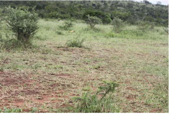
Figure 1. Grazing lawn in HiP
The lawn in the front is characterised by a short grass height due to horizontal growth. In the back-ground, where the grazing lawn ends, tall bunch grass dominates.
To be maintained, grazing lawns need to be exposed to continuous grazing in order to remove tall grass that might invade and to stimulate growth (Georgiadis et al., 1989; Hempson et al., 2014). Although white rhino is considered to play a key role here (Owen-Smith, 1988), other grazing mammals like impala (Aepyceros
melampus) also seem to be able to maintain lawns (Cromsigt and Olff, 2008) at least
in low rainfall areas (Waldram et al., 2008). Because grass on grazing lawns requires a monthly rainfall of 25 mm to grow, the usage of this food resource is usually limited to the wet and the beginning of the dry season when precipitation or soil moisture is relatively high (Bonnet et al., 2010; Hempson et al., 2014).
Fire is also a consumer of grass biomass and is able to reduce biomass remarkably within days (Archibald and Hempson, 2016). Instead of treating them as independ-ent processes, research has shifted its focus to studying the interaction between fires and grazing (Archibald et al., 2005). Because the potential fuel load on grazing lawns is low, these areas do not burn usually (McNaughton, 1992; Archibald et al., 2005; Leonard et al., 2010). Instead, fire removes senescent tall grass, is able to stimulate grass growth and in addition, the regrowth after a burn offers a high ent content mainly due to a high leaf to stem ratio, young plant material and a nutri-ent distribution among a small amount of biomass (Vesey-Fitzgerald, 1971; Van de Vijver et al., 1999; Donaldson et al., 2018). Thus, regrowth is high in N, Cu, K and
Mg content during the first two months after a fire (Eby et al., 2014). Many African grazing ungulates are known to be attracted by burnt grassland to take advantage of it (Moe et al., 1990; Archibald et al., 2005; Donaldson et al., 2018). Earlier obser-vations also suggest a positive response of white rhinos to burnt areas (Owen-Smith, 1988; Shrader et al., 2006), although their preference has yet to be intensively tested. This study investigates how white rhinos respond to fire during the dry season, when grazing lawns do not provide enough food. As mentioned above, white rhino can tolerate low quality food and tall grass (Owen-Smith, 1988; Perrin and Brereton-Stiles, 1999), yet they still prefer high quality food whenever available, since they use the nutritious grass on grazing lawns and tend to favour short grass over senes-cent tall grass also during dry season if available (Arsenault and Owen-Smith, 2008). Thus, I would expect that white rhinos will positively respond to burnt areas. The territories of dominant males usually contain both grazing lawns and tall grass areas and therefore seem to contain foraging habitat for every time of the year (Owen-Smith, 1975). If rhinos use burnt areas during the dry season, then frequent burns may be a crucial feature of good habitat and I would expect that long-term habitat selection is influenced by burn frequency. Other studies have shown a long-term preference for frequently burnt grasslands for other herbivorous mammals like impala, wildebeest and zebra (Equus quagga) (Burkepile et al., 2013; Donaldson et al., 2018).
The relevance of this study reaches beyond expanding scientific knowledge. Its re-sults should be a first step towards protecting white rhinos more efficiently against poaching. A better understanding of rhino movement and spatial/temporal concen-trations of individuals as driven by burns would enable anti-poaching units to focus their patrols on spatiotemporally-specific rhino hotspots. In addition, park manage-ment could burn areas least accessible to poachers to concentrate white rhinos in those areas.
In this study I investigated the short-term response of the white rhino to burns during dry season as well as the degree to which fire frequency impacts long-term white rhino distribution. I formulated the following hypotheses:
1) During the dry season, white rhino shows a positive response towards burnt areas a few weeks after a fire.
2) White rhino’s habitat and territory selection is impacted by fire frequencies and thus, long-term rhino density is higher in areas with frequent burns.
2.1 Study site
The study was conducted in Hluhluwe-iMfolozi Park (HiP), a game reserve in Kwa-Zulu-Natal in eastern South Africa (Figure 2). It extends over an area of 96 000 ha, running from 28°00’S to 28°26’S and from 31°43’E to 32°09’E (Whateley and Por-ter, 1983; Cromsigt and Olff, 2006). Variation in altitude leads to considerable spa-tial variation in annual rainfall between higher (annual rainfall about 985 mm) and lower regions (650 mm) (Cromsigt and Olff, 2006).
Figure 2. Hluhluwe-iMfolozi Park (HiP) in South Africa
Left: HiP is located in KwaZulu-Natal (light orange) in eastern South Africa. Right: The Park is di-vided into five sections, two are located in Hluhluwe (green) and three in iMfolozi (orange).
In general, due to the difference in altitude, Hluhluwe receives more precipitation annually than the southern region of iMfolozi. Rainfall occurs mainly during south-ern hemisphere summer and therefore starts in October and ends in March usually (Howison et al., 2017). Due to a combination of climatic drivers, fire and herbivory, vegetation and habitat type vary considerably throughout the park. The habitats are broadly classified as; forests, thickets, woodlands, open woodlands and grasslands all being found across the region (Whateley and Porter, 1983).
Two aspects render HiP particularly suitable for the question of this study. Firstly, HiP has a long history of prescribed fire regimes and documentation started already in the 1950s. Historically, fire management has been very intensive with a median fire return interval of 1.3 years (Balfour and Howison, 2002; Archibald et al., 2005) and intended burns still occur almost every year. Secondly, HiP has among the highest white rhino densities worldwide. After population size has de-clined to a minimum of 100 to 200 individuals at the end of the 19th century,
num-bers started to increase in the 1920s (Owen-Smith, 1975) up to over 2,000 individ-uals during the late 2000s (Le Roux et al., 2017).
2.2 Data acquisition and preparation
In order to conduct analyses over large temporal scales, I used both pre-existing and newly collected data. This included data about white rhino, fire and other environ-mental features on individual burns or within grid cells (3km2) that were used in the
analyses. The following sections describe data type, structure, acquisition and prep-aration.
2.2.1 White rhino distribution
In order to analyse white rhino distribution, I used a long-term ungulate census data set provided by the park management authority, Ezemvelo KZN Wildlife (EKZNW). The census has been run since 1986 on a biennial basis and covers 34 line transects throughout the park, totalling 281 km. During each census event, run during the period July – October, each transect is walked by one observer and an armed guard, ideally more than 15 times. Every ungulate observed within 500 m to each side of the transect is recorded, noting the species, group size, date, the coor-dinates of the observer, sight distance and bearing to the animal and whether the observed animal was on a burnt spot or not. From the sighting distance and bearing, perpendicular distance between transect and the animal is calculated using Pythag-oras’ theorem. This information I then used to calculate distance derived density estimates (see 2.3.1). In this study, I used white rhino census data recorded between
2002 and 2014, totalling 7 census counts (2002, 2004, 2006, 2008, 2010, 2012, 2014). Using the coordinates of the observer and both sighting bearing and distance, I determined the actual location of each animal.
2.2.2 Fire occurrence in HiP
Reliable fire maps including both temporal and spatial information were a crucial requirement for all of the following analyses. Three different long-term data sets that provide information about burns in HiP were available, each with different res-olutions and associated errors.
First, section rangers produce yearly park maps that show the spatial extent of fires. Generally, these maps include information on the start and end date for each burn, although this information were at times missing or vague. I used yearly man-agement fire maps from 2002 – 2017.
The second data set consisted of Collection 6 MODIS Burned Area Product (Gi-glio et al., 2015) (hereafter MODIS) that was downloaded in September 2018 from ftp://ba1.geog.umd.edu for each year between 2002 and 2017. It is based on the MCD64A1 burned area mapping algorithm and relies on surface reflectance and active fire input data. Monthly produced maps at a resolution of 500 m contain rec-tangular polygons that indicate a burn. Every polygon is equipped with a burn date in the day-of-year format (Giglio et al., 2016). This means, that Jan 1st is day one while Feb 2nd is day 32. For consistency, this format was adopted for every data set and analysis. In order to reduce file size and amount, monthly MODIS maps were cut corresponding to the outer boarders of HiP and merged per year using QGIS version 3.4.
Third, the ungulate census also included information about fire as mentioned above. Although this data set did not delineate burnt area borders, it still gave some evidence for or against a fire event on a particular location at a certain time. I used the census counts from 2002, 2004, 2006, 2008, 2010, 2012 and 2014.
Unfortunately, comparison of the three data sets detected remarkable discrepancies and each set showed some weaknesses. Therefore, I did not find it reasonable to trust in one data set exclusively. Instead, I created yearly fire maps by combining all three data sets as explained below (Figure 3- Figure 6). First of all, I transformed MODIS fire data into a convenient and manageable form by amalgamating the large amount of polygons into single burn events based on temporal and spatial proximity. Start and end date were provided for every burn event by considering the earliest and latest burn segment within the amalgamated polygon(Figure 3).
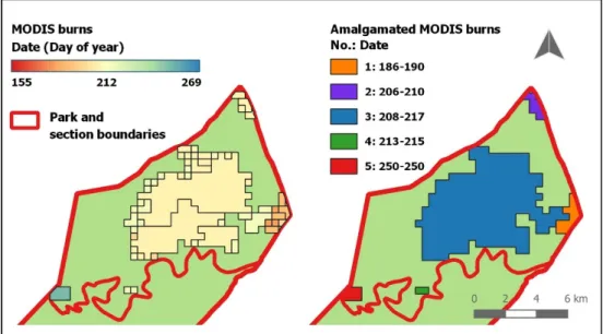
Figure 3. Amalgamation of MODIS polygons in Manzibomvu section during 2014
Left: Original MODIS data is shown as single polygons, each equipped with an individual burn date (gradually coloured). Right: Single polygons were amalgamated and form spatially connected burns when start and end date were shared.
In the next step, I included park management maps. In the case of an overlap be-tween MODIS recorded burns and park management recorded burns, this overlap was confirmed as the spatial extent of a burn. If, in addition to that, both data sets presented not only spatial congruence but temporal comparability, the confirmation of this particular burn was complete. However, in the case of temporal discrepancies between the overlap of these two data sets, I used the third data set (burn information within the ungulate census database) to resolve these discrepancies. Because the census records included information on whether or not the animal was observed on a burn on a certain date, this could be used to validate the burn date (Figure 4). Besides the actual animal observations, the date on which a transect was walked could also be taken into account to specify a burn date, because it is very unlikely that someone walked through an area while it was burning. After the analysis of spatial overlapping areas was completed, areas that are identified either by MODIS or the park maps still needed to be evaluated. Again, I used the data from the ungu-late census for validation. If they supported a burn, it was adopted and vice versa (Figure 5). Finally, some polygons remained, which were suggested as burnt by only one spatial data set but without census records available to verify. Here, I based my decision for or against the acceptance of a burn on the overall performance and re-liability of the different data sets. For example if one of the data sets suggested a burn, but was, in the past, found to be inaccurate and tended to overestimate the burn extent (as shown by census records in previous steps), then a decision was made to ignore the burn event.
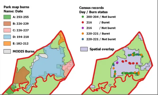
Figure 4. Example of overlap between Park management maps and MODIS
Left: Amalgamated MODIS burns (light grey) were overlaid with park management recorded burns (coloured according to date). Right: Spatial overlapping areas (dark grey) needed to be further veri-fied if temporal information did not match (Compare park map burn D (blue, left) and MODIS burn 3 from Figure 3). For this particular burn, census records (points) indicate a fire event between day 205 and 215. This date was thus finally adopted.
It is important to mention that a gen-eral conclusion about the performance of one of the data sets was not possi-ble, because data quality differed be-tween years and sections. These tem-poral and spatial quality differences are probably caused by continuous ad-justments of MODIS fire detection, differences in cloud cover that influ-ence detection probability and varying effort that was made in terms of the production of the park management fire maps. Therefore, I evaluated the reliability of each of these questiona-ble burns on a case by case basis. If in the end, it was still not possible to make a defensible decision for or against a fire occurrence, a burn was accepted.
Figure 5. Example of spatial differences between MODIS and park management map
Areas that were recorded to have burnt by only one data set (i.e. according to either MODIS (rose) or park maps (orange)), were analysed by census rec-ords. If the majority of records supported the occur-rence of a burn (blue), the area was treated like a burn.
In a last step, I merged all finally con-firmed burns including information on burn start and end date to one fire map per year (Figure 6). Following this described approach, fire maps were produced for the entire park for every year, in which census data were available. For the years in between, I merged MODIS burns and park man-agement recorded burns to obtain spatial fire extent per year. Their us-age was limited to the fourth part of the study (see 2.3.4) which deals with long-term response to fire. For this purpose, only the frequency of burns in a given area but not the exact date of a burn was of interest. Therefore, a verification of burn dates was not nec-essary.
2.2.3 Grazing lawn occurrence in HiP
In 2004, 2010 and 2014, the same transects that are used by the ungulate census were walked in order to document the amount of grazing lawns next to the transect. A grazing lawn was recorded whenever more than 75% of the grass in each 5 by 10 m plot along the transect consisted of grazing lawn species maintained in a grazing lawn stature. Grazing lawn species were identified due to a horizontal or dwarfed growth form and a lawn stature was characterized by a short grass height without vertical outgrowth. For this study, I calculated the proportion of grazing lawn on a transect by dividing the amount of lawn (measured in meter along transect) by length of the transect. Some transects were walked in 2014 only. In these cases, I adopted measurements from 2014 for 2004 and 2010. For years, in which grazing lawns were not measured, I used the measurement closest in time (e.g. measure-ments from 2004 were used for 2006, see Table 1). In October and November 2018, I also measured grazing lawns along roads, using two observers (in addition to the driver) in a car to record lawns on both sides of the road. An area needed to fulfil the same requirements as during the census transect measurements to be included as a grazing lawn. We drove 216 km (Figure 7) at an average speed of about 10 km/h. Again, I calculated grazing lawn proportion by dividing recorded lawn length by sample effort in meters.
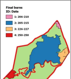
Figure 6. Finally confirmed individual burns in Manzibomvu in 2014
Every burn that was identified during the previous steps was equipped with an ID and a date for burn start and end.
Table 1. Overview of the usage of graz-ing lawn measurements
Because grazing lawns on transects were recorded in 2004, 2010 and 2014 only, the measurements closest in time were used for the analysis of years with-out records.
Analysed year Used grazing lawn records (Year) 2002 2004 2004 2004 2006 2004 2008 2010 2010 2010 2012 2014 2014 2014 2.2.4 Precipitation in HiP
The amount of precipitation in different parts of the park is mainly driven by differ-ences in elevation (Balfour and Howison, 2002). To get a spatial information of rainfall, I used a 250 m resolution rainfall interpolation map produced by Howison et al. (2017) which was based on elevation and monthly rainfall measurements be-tween 2002 and 2007 from 17 rainfall stations representing the general spatial rain-fall differences (Howison et al., 2017; Le Roux et al., 2019). Using this map, I calculated the relative spatial differences in rainfall between individual burns and between grid cells by centralizing the interpolation values. To obtain a temporal rainfall trend, I used rainfall records from the five stations with the most exhaustive records (Masinda, Nqumeni, Research, Mbhuzane, Makhamisa) to calculate aver-age rainfall in HiP for each hydrological year (July - June) between 2001/2002 and 2013/2014. I calculated burn-specific annual rainfall by multiplying temporal rain-fall estimate by the spatial rainrain-fall estimate.
2.2.5 Midden count
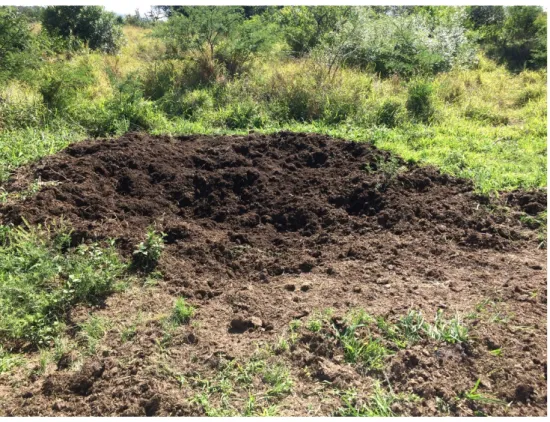
I used middens as an indicator for long-term rhino density. Middens are dungheaps (Figure 8) that are produced by frequent defecation of a dominant male, females, sub adults and subordinate males, last for many years and are very abundant in white rhino habitats (Owen-Smith, 1975). I recorded white rhino middens throughout the
Figure 7. Road transects in 2018
Roads (black lines, 216 km in total) were driven in a car in order to measure grazing lawns. The southern part of HiP was not covered due to inaccessibility.
park on the above mentioned road transects (see 2.2.3) and took the GPS location for each midden. In order to take into account a declining detection probability with increasing distance to the road, only middens within 20 m were recorded. In case of doubt, the distance was measured using a range finder.
Figure 8. White rhino midden in HiP
2.3 Data analysis
I performed four analyses in this study. Firstly, I used rhino census data from 7 years to estimate rhino abundance on the same transect segments before and after a burn during the same season using distance sampling techniques (see 2.3.1). These esti-mations were used in the second analysis to test, if rhino abundance increased sig-nificantly after a burn (see 2.3.2). This analysis informs us about short-term rhino response to burnt areas after the first weeks following a burn. For the third analysis, I again compared the same pre- and post-burn rhino abundance estimates as in the second analysis but now using a generalized linear mixed effect model (GLMM) where I also included other environmental predictors of white rhino distribution in addition to fire (see 2.3.3). This analysis informs us whether the response of rhino to burns may depend on other environmental variables. In the fourth analysis, I used the midden counts to test whether fire frequency (between 2002 and 2017) has an
impact on long-term rhino distribution (see 2.3.4). The software QGIS version 3.4 and R version 1.1.463 were used for all analyses and data preparation.
2.3.1 Rhino abundance estimation
In order to estimate pre- and post-fire rhino abundance, I identified those parts of a transect that burnt (hereafter called burnt segments) by using the yearly fire maps produced before. Segments needed to fulfil two requirements to be included in the analysis: First, only segments with a size of at least 0.5 km² were included in order to avoid the overestimation of single rhino observations or the absence of observa-tion on very small segments. Second, a transect segment needed to be walked (in terms of census counts) at least four times both before and after a fire event. In order to guarantee equal sample size before and after a fire for each segment, I subset the data for each segment to include the same amount of pre- and post-fire census walks to estimate rhino abundance. Whenever a subset was chosen out of a larger number of potential census walks, I used the walks immediately prior to the fire event for pre-fire measurements. In contrast, for post-fire measurements, the last census walks were chosen, allowing for the maximum amount of time between fire and the census counts to allow for maximum grass post-fire regrowth. Thus, the post-fire census walks used here were conducted on average 3 weeks after a fire event. In the end, 54 burnt transect segments fulfilled those requirements.
I used a distance sampling approach (Buckland et al., 1993), whereby density is estimated by calculating the change in detection probability with the perpendicular distance from the transect line. This function can be described as a fall-off curve and takes into account, that the probability to detect an animal might depend on the distance to the observer (Miller et al., 2017). Fire obviously leads to an increased visibility due to the removal of tall grass and leaves of shrubs. Thus, the detection curve is likely to be different between a pre- and a post-fire environment. Therefore, I divided the data set into one subset including before and another subset including after burn observations. The ‘Distance’ package (Miller, 2017) which extends the ‘mrds’ package (Laake et al., 2018) was used for distance sampling analysis in R. The function ‘ds’ searches for a detection function and calculates the average prob-ability to see an animal. A general assumption is that animals are evenly distributed across the study area (Miller et al., 2017). In order to avoid a density inflation on the transect line (and therefore at a perpendicular distance of 0 m), records at a dis-tance < 1 m were truncated. I tested various detection functions (both half-normal and hazard-rate key functions, each with cosine, hermite polynomial and simple polynomial adjustments). For each combination of key model and adjustment, the
optimal amount of adjustment terms were selected according to Akaike’s Infor-mation Criterion (AIC) (Miller et al., 2017). For the purpose of model selection, I produced quantile-quantile-plots comparing fitted and empirical distribution func-tion. Beside this visual approach, the goodness of fit was calculated by using the Cramér-von Mises test for each selected model. It tests how well model predictions match the underlying data (Miller et al., 2017). A p value < 0.05 indicates that the null hypothesis, which says that the data derived from the model should be rejected. Thus, only models with a p value > 0.05 were kept. Out of the remaining models, I selected the best based on the lowest AIC (Burnham and Anderson, 2003). It is good practice to select the simplest model, if AIC values differ by less than 2 (Miller et al., 2017). In the end, I used the selected model to calculate both rhino abundance and density for every segment before and after a burn for use in the next analyses.
2.3.2 Comparison of pre- and post-fire rhino abundance
The abundance estimations for white rhinos on the same transect segment before and after a burn obtained in the first analysis were used here. Because of non-nor-mality, I used the Wilcoxon’s signed rank test to test for significant differences in pre- and post-fire rhino abundance. A visual inspection was conducted using a box-plot.
2.3.3 Impact of burns on short-term rhino distribution
The following analysis should test, if burns alone can explain differences in rhino abundance or whether other environmental factors are crucial. Since the design of the study included count data originating from repeated measurements and both fixed and random effects, I chose a generalized linear mixed effect model (Crawley, 2007). I used abundance as response with the logarithm of segment size as an offset and explanatory variables included a) the presence or absence of a burn (categori-cal), b) logarithm of precipitation during the hydrological year, c) proportion of burn within a buffer of 1.5 km around the burnt segment and the d) proportion of grazing lawn on the corresponding transect (all continuous). Additionally, the interaction between e) burn and precipitation was included. The proportion of burns within a buffer of 1.5 km around the segment was calculated based on the fire maps. I chose this particular size of the buffer because a distance of 1.5 km has been shown as a spatial threshold up to which others grazers are attracted by fire (Archibald et al., 2005). Since abundance is influenced by area size (which was dealt with using the offset term in the model), I used density to identify outliers instead. Outliers that need to be excluded were defined as being 3 times the interquartile range above and below the third and first quartile respectively and were removed from the data set
(Crawley, 2007; Ghasemi and Zahediasl, 2012). I tested explanatory variables for variance inflation (collinearity) using the ‘vif’ function, which is part of the ‘car’ package (Fox and Weisberg, 2011). A VIF value larger than 3 was used as cut-off value (Zuur et al., 2009) and therefore the proportion of burn within the buffer was removed. The recalculation for the remaining variables led to values that were even lower than a very strict cut-off of 0.5 (Booth et al., 1994) and were therefore kept. The GLMM analysis was conducted using the function ‘glmer’ out of the ‘lme4’ package (Bates et al., 2015). First, a full fixed effect model was run, specifying a poisson family. Segment-ID nested within Transect-ID was defined as random ef-fect. Afterwards, a control structure with the optimizer ‘bobyqa’ needed to be con-structed to enable the model to converge. I checked the model for overdispersion. For validation of the full fixed effect model, I plotted residuals against fitted values. Residuals were also plotted against each explanatory variable to check heterosce-dasticy (non-constancy of variance (Crawley, 2007)). Only the plot for the variable burn seemed to be slightly suspicious. Hence, Bartlett and Fligner-Killeen tests were conducted in order to investigate this further. Both tests indicated that heteroscedas-ticy was not an issue and therefore the analysis was continued. Once the random component was defined, the optimal fixed effect structure was obtained by sequen-tially removing the non-significant explanatory variable (p > 0.05) with the highest p-value. Then, the new model was run again. I continued that until only significant variables remained. Following the approach for model selection suggested by Bolker et al. (2009), I calculated AIC values for every model and chose the one with the lowest value.
2.3.4 Long-term effect of fire on rhino abundance
This part of the study looked at the impact of long-term fire frequency on long-term rhino distribution (as measured through midden density along roads). I overlaid the park with a raster of grid cells with a size of 3 km² and used those, which were covered by the road measurements (Figure 9). The number of middens within a grid cell was used as response with the logarithm of the measured road length as an off-set. Explanatory variables were a) lawn cover, b) the centralised spatial estimate of precipitation, c) fire frequency, d) average fire proportion (in relation to cell size) and an interaction between e) fire frequency and proportion. In comparison to the second analysis, I did not have any random effect and therefore, I chose a general-ized linear model (GLM). The analysis was conducted by using the ‘glm’ function
out of the R-package ‘stats’. Model validation and selec-tion was done similar to those conducted in the GLMM during the second analysis (see 2.3.3). I used cook distance to check for a large influence of single ob-servations and a distance larger than 1 was used as the critical threshold (Fox, 2002; Zuur et al., 2009). When differences in AIC values for the models ob-tained were smaller than 2, I used model averaging (Burnham and Anderson, 2003; Zuur et al., 2009). Figure 9. Fire frequency in grid cells (3 km²)
Fire frequency (gradually coloured) varies between 1 and 14 burns during 2002 and 2017 in cells that were analysed.
3.1 Rhino abundance estimation
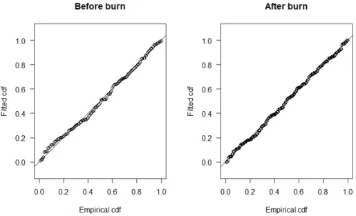
The before and after burn detection functions were best described through a hazard-rate model with a cosine adjustment. The visual inspection via quantile-quantile-plot (Figure 10) indicated a good fit between the models and the data. The Cramér-von Mises test, which tests the goodness of fit, provides p-values of 0.8653 for be-fore burn and 0.9788 for after burn observations. Values higher than 0.05 give evi-dence that the model fits the data (Miller et al., 2017).
Figure 10. Quantile-quantile-plots for selected detection functions
Plots compare the cumulative detection function (cdf) of the fitted detection function with the distri-bution of the actual observation indicating how well the models fit. The closer the points to the line, the better the model. Thus, the hazard-rate model that was chosen here fits well both for before burn and after burn observations.
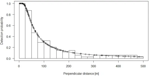
The fitted detection functions provide the probability to detect a white rhino at a given distance on a transect. With increasing distance, the detection probability drops faster in unburnt areas than in burnt areas (Figure 11and Figure 12).
Figure 11. Detection function for white rhino prior to a burn
The probability to detect a rhino drops drastically with increasing distance to the transect. Bars rep-resent actual observations at a given perpendicular distance.
Figure 12. Detection function for white rhino after a burn
Detection probability with increasing perpendicular distance after a burn does not drop as fast as prior a burn (compare Figure 11)
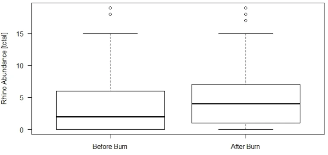
3.2 Comparison of pre- and post-fire rhino abundance
The abundance of white rhinos on the same transect segment during the same season increased slightly after a burn (Figure 13). According to the Wilcoxon’s signed-rank test, the observed differences were significant (p = 0.03752).Figure 13. Boxplots showing differences in white rhino abundance on the same transect segments before and after a burn during the same season and year
Median rhino abundance increased slightly after a burn. The observed difference is significant (p = 0.03752, n=54).
3.3 Impact of burns on short-term rhino distribution
The model that fits to the data best is a one-factor model with burn category as the only remaining explanatory variable. Burn had a significantly positive impact on rhino abundance (Table 2), suggesting that rhino abundance increased on the same transect segment following a burn. All other variables (precipitation, proportion of grazing lawns on transect and the interaction between burn and precipitation) did not explain any of the variation in rhino abundance and were removed sequentially (Table 3).
Table 2. GLMM for white rhino abundance
Burn category is the only remaining explanatory variable that has a significant impact (p < 0.05) on rhino distribution.
Estimate SE z-value p-value
Intercept -0.08289 0.18216 -0.455 0.6491
Table 3. Overview of removed explanatory variables
Variables were removed sequentially due to the lack of significance.
Estimate SE z-value p-value
Burn:Precipitation -0.2463 0.8602 -0.286 0.775
Lawn cover 2.51952 3.63976 0.692 0.4888
Precipitation -1.47183 1.19093 -1.236 0.2165
3.4 Long-term effect of fire on rhino distribution
All candidate models differed only slightly in their AIC values (Table 4). Therefore, all models with a delta AIC of < 2 were averaged. Model averaging estimates are reported in Table 5. The averaged GLM indicates that lawn cover is the only varia-ble that has a significant influence on the amount of middens representing rhino long-term distribution within a grid cell. Both fire frequency and proportion re-mained within the best supported model, but their averaged estimates were not sig-nificant. Models containing precipitation and the interaction between fire frequency and proportion were not supported (delta AIC > 2).
Table 4. Overview of models obtained during GLM analysis
5 models were tested (x indicates variable inclusion). The model with the lowest AIC value and those with an AIC difference smaller than 2 were averaged in the next step (Here M4, M5, M3).
Model Lawn cover Precipita-tion Fire fre-quency Fire pro-portion Fire fre-quency:Fire proportion AIC ΔAIC M4 x x 497.0901 M5 x 497.8379 0.7478 M3 x x x 498.3567 1.2666 M2 x x x x 499.7114 2.6213 M1 x x x x x 501.0283 3.9382
Table 5. Averaged GLM for long-term distribution of white rhino
Lawn cover has a highly significant impact (p < 0.001) on rhino distribution. The other remaining explanatory variables are not significant.
Estimate SE z-value p-value
Intercept -6.46057 0.17434 36.835 < 2e -16 ***
Lawn cover 1.36940 0.34034 3.983 6.8e -05 ***
Fire proportion -0.42459 0.28224 1.489 0.137 Fire frequency -0.01529 0.01783 0.848 0.396
This study provides evidence that fire has a significant positive effect on white rhino abundance at a short-term scale and might be a thus-far underestimated driver of short-term rhino habitat selection. During the analyses of data from seven years, rhino abundance increased significantly three weeks after a fire (average of tested temporal distance) and neither precipitation nor the amount of grazing lawns nearby were able to explain differences in white rhino abundance. Thus I found support for my first hypothesis, that white rhinos show a positive response towards burnt areas. My results do not support the second hypothesis, that fire frequencies influence long-term habitat and territory selection and that rhino density is higher in areas with frequent burns.
The results contradict the findings of Sensenig et al. (2010), who observed a low burn preference of large herbivores and hindgut fermenters, which is both true for white rhino. This discrepancy is less surprising if one considers, that white rhino has already been shown to be an exception regarding the relationship between body size and favoured diet (Kleynhans et al., 2011). The general pattern indicates, that large herbivores can tolerate and utilize food resources of low quality whereas smaller ones rely on a high quality diet and thus, resource partitioning is based on body size (Illius and Gordon, 1993). The megaherbivore white rhino does not fit in this pattern and feeds on short grass higher in quality than expected (Kleynhans et al., 2011). This can be explained by the wide muzzle of white rhinos. This morphological feature enables the rhino to take in a sufficient quantity despite the short sward, where other large grazers cannot obtain large enough quantities (Arsenault and Owen-Smith, 2008). The results of my study support this view of white rhino being an exception to the above mentioned pattern. Therefore it might be worth to continue further investigations dealing with interspecies competition on burns.
The results indicate that white rhino’s preference for burnt areas is independent from the amount of precipitation. At this point it should be mentioned that the results obtained in this study hold true for HiP and its rainfall ranges. HiP is a relatively
mesic savanna with an average annual rainfall between 650 mm and 985 mm depending on altitude (Cromsigt and Olff, 2006). Precipitation might be influential in other parks or regions with different rainfall ranges. However, white rhino’s response to fire could be influenced by environmental properties other than precipitation, like vegetation type and soil composition or by rhino density, aspects that might differ in other parks. Therefore one should take care when it comes to generalizing the results of this study. They describe observations in HiP and may not be true for white rhinos in different ecosystems.
The positive response of white rhino to fire observed here is significant but not immense. This study may have benefited from the inclusion of more data which might have unmasked an even stronger response. In addition, the census count used here did not distinguish between feeding and, for example, resting individuals. Thus, it might be reasonable to include only grazing animals because resting rather occurs in shady areas or mud wallows than on grassland (Owen-Smith, 1975). Alternatively, the response area in which rhinos were counted (here the burn itself) could be expanded by including a buffer of a certain size around the burn. Finally, it is reasonable to consider reasons other than high food quality that could play a role in terms of rhino’s preference for burns. The avoidance of parasites might be an additional factor that makes a burnt area beneficial (Fyumagwa et al., 2007). While this study indicates that fire has an impact on white rhino distribution at a small time-scale, I did not find any evidence that it influences habitat selection in the long term. One could argue, that fire might have an impact in parks where burns occure less frequently than in HiP. But since the analysed grid cells represented a high variation in terms of fire occurrence and also areas with very low fire frequencies, I do not assume that a selection was masked by the lack of frequencies below a critical threshold. However, many neighboring grid cells have experienced very similar fire frequencies. This reduced variation of frequencies on a smaller spatial scale might have prevented habitat selection based on fire history. Grazing lawn cover was the most important habitat feature that shaped long-term rhino distribution. Nevertheless it should be noted that in this particular case it is difficult to separate cause and effect. Since grazing lawns are initiated and maintained by white rhino, high grazing lawn cover might be an indicator for rhino abundance rather than the cause of rhino presence. In addition, the numbers of middens alone might have been an insufficient indicator of long-term rhino presence, since the same midden can be used by one or many individuals. Other midden characteristics like size may provide a better insight. These insecurities about how to use middens is probably one reason, why white rhino is often excluded in studies that deal with grazer’s presence. While many experimental designs rely on dung counts, this approach becomes difficult, as soon as one wants to include rhinos (Archibald et al.,
2005). Therefore, detailed investigations about the potential usage of middens could be the door-opener for many further rhino related studies. Different habitat features than those included in this study could be important to predict long-term rhino presence. Potential candidates are water availability or slope, for example (Perrin and Bereton-Stiles, 1999). Finally, the effect of frequent fires on rhino presence may also should have been hypothesized to be negative. It has been shown, that fires can drive the development and establishment of nutrient-poor tall grass areas in an ecosystem (Archibald et al., 2005). However, neither a positive nor a negative long-term response to frequent fires has been found here. If there is an interaction between long-term habitat selection and fire, it might be more complex than the pattern of fire frequency and size. Patchiness of a fire, fire return interval and severity might be worth to consider in further studies.
This study faced some limitations which are worthy of addressing in future related studies. The uncertainty of the accuracy of fire records should be reduced to obtain more reliable maps. One approach to improve the fire maps could be the mapping of fire scars via drone images and a more accurate and complete documentation of burn dates. Another possibility is the use of satellite images with a higher resolution. Regardless, one robust fire map may be more reliable than combining three data sets in an effort to correct for the weaknesses of each. Finally, fine scaled fire maps would give the opportunity to answer research questions that are beyond those of this study. For example, one application could be to investigate whether white rhino shows a stronger response towards burnt patches of a certain size. In comparison to large burnt patches, small patches offer rather high quality food with a high portion of live leaf material and a low percentage of acid detergent fibers, because small patches are easier to maintain in a short state by grazers (Sensenig et al., 2010). In general, there is some evidence that African herbivores are attracted more by small burnt patches (Sensenig et al., 2010; Donaldson et al., 2018). This is particularly true for small animals, while herbivores with a large body size tend to favour larger burnt areas (Sensenig et al., 2010). Again, this observation supports the pattern that smaller animals search for high quality food in opposite to large ones. Like discussed above, this is not entirely true for white rhino and it would be interesting to check whether this anomaly can be found again. A very different approach to the one used in this study could be a real time study in which one observes individual burns on a daily basis. This would provide very fine scaled information about time-dependent preferences. Grass tends to sprout already about one week after fire (Hopkins, 1965), but this might be also influenced by soil moisture, which depends on rainfall during the previous season and precipitation during the fire season. While this study tested for a positive response to fire after a few weeks, further studies could test the hypothesis that white rhino will use burnt grassland intensively
already within the first week after a fire. This has been reported for other herbivores in former studies (Moe et al., 1990). In addition, some herbivores have been observed on burnt areas even immediately one day after a fire, probably in order to take advantage of the ash being rich in Ca, K, P and trace minerals (Komarek, 1969). That could be true for white rhino as well. Another open question is whether the response to burns differs between males and females. Dominant males are restricted to their territories with an average size of about 1.65 km² while females, sub adults and subordinate males have a more or less wide range to forage (Owen-Smith, 1975). Therefore one can assume that dominant males show a weaker response than the others. In order to answer this question, a rhino data set that includes sexual information is necessary.
Ideally, the findings in this study and further ones can be used to protect white rhinos more efficiently against poaching. A knowledge about factors that impact rhino movement at a small time scale enables anti-poaching units to focus their patrols on spatiotemporally limited rhino hotspots. This would be optimized if one investigated, up to which distance white rhinos are attracted by burns. The observation that grazers leave their usual foraging habitat due to the attractiveness of nearby burns has been described as ‘magnet effect’ (Coppock and Detling, 1986). This effect depends on the distance of the burn to the area used before. It has been shown, that herbivores are drawn off from their usual grazing place within a distance of 1.5 km to a burn (Archibald et al., 2015). A similar distance could be assumed and tested for white rhino.
Lastly, fire might affect not only anti-poaching activities, but rhino poaching can also influence fire. Grazing lawns, which reduce the amount of potential fuel remarkably, are considered to be able to prevent and break fires (McNaughton, 1992; Archibald et al., 2005; Leonard et al., 2010). Hence, reduced numbers of white rhino could lead to more frequent and less patchy fires, which supports the development of tall grass (Archibald et al., 2005). Thus, rhino poaching might not have a negative effect exclusively on white rhino but results also in a complex cascade of effects on ecosystems and their grazers.
For millions of years, fire has impacted human being’s life. While it might be scary on the first sight, people learned how to deal with fire. When we think about fire, we might associate fear, fascination or fun. And animals? We can only guess, what they think about fire. But we can investigate, how they respond. And this response is by far more than escaping from it.
Pyrophile beetles lay their eggs under the bark of burnt trees, some Australian birds are suspected to spread fires intentionally to chase predators away and different African grazers are known to search actively for burnt parts of the savanna in order to feed on the nutrient rich post-fire regrowth. The latter is true for wildebeest, impala and zebra for example. But how does the white rhino, maybe the most fascinating grazer of the African savanna, respond to fire? Its favoured diet consists to a large part of grass from grazing lawns, a grassland type characterized by very short and nutritious grass due to a high amount of leaves. But this high quality food resource is available during the wet season only because regrowth requires a certain amount of rainfall. Good news for white rhinos: They are able to digest food of low quality and therefore, they can use senescent tall grass during the dry season. But if there is an area available that has burnt recently, will white rhinos use the nutrient-rich grass although they do not have to? This study has investigated long-term data sets about fire and rhino distribution in the Hluhluwe-iMfolozi Park in South Africa and has observed a preference of white rhino for burnt areas. Indeed, fire was the only habitat feature tested that was able to explain differences in rhino abundance. Nevertheless, many questions still remain unanswered: This study did not find any evidence, that fire drives habitat selection on a long-term. In addition, it is still uncertain how fast rhinos respond to fire, up to which distance they are able to detect a fire and whether certain characteristics of a fire are more beneficial than others. A good understanding of rhino movement in response to fire would enable the park managements to protect the white rhino efficiently against poaching. Intensive poaching and the reduction of suitable habitats have led to a reduction of rhino
numbers. Now is the time to investigate in further studies, how fire and white rhino interact. One thing is likewise obvious and sad. While fire will outlast humankind by million years, white rhino will not.
Anderson, T.M., Dong, Y. & McNaughton, S.J. (2006). Nutrient acquisition and physiological responses of dominant Serengeti grasses to variation in soil texture and grazing. Journal of Ecology, vol. 94 (6), pp. 1164 - 1175.
Anderson, T.M., Kumordzi, B.B., Fokkema, W., Fox, H.V. & Olff, H. (2013). Distinct physiological responses underlie defoliation tolerance in African lawn and bunch grasses. International Journal of Plant Sciences, vol. 174 (5), pp. 769 - 778.
Archibald, S., Bond, W.J., Stock, W.D. & Fairbanks, D.H.K. (2005). Shaping the landscape: Fire-grazer interactions in an African savanna. Ecological Applications, vol. 15 (1), pp. 96 - 109. Archibald, S. & Hempson, G.P. (2016). Competing consumers: contrasting the patterns and impacts
of fire and mammalian herbivory in Africa. Phil. Trans. R. Soc. B., vol. 371 (1703), 20150309. Arsenault, R. & Owen-Smith, N. (2008). Resource partitioning by grass height among grazing
ungulates does not follow body size relation. Oikos, vol. 117 (11), pp. 1711-1717. Balfour, D.A. & Howison, O.E. (2002). Spatial and temporal variation in a mesic savanna fire
regime: responses to variation in annual rainfall. African Journal of Range and Forage Science, vol. 19 (1), pp. 45 - 53.
Bates, D., Maechler, M., Bolker, B. & Walker, S. (2015). Fitting Linear Mixed-Effects Models Using lme4. Journal of Statistical Software, vol. 67, pp. 1 - 48.
Bolker, B.M., Brooks, M.E., Clark, C.J., Geange, S.W., Poulsen, J.R., Stevens, M.H.H. & White, J.S. (2009). Generalized linear mixed models: a practical guide for ecology and evolution. Trends in ecology & evolution, vol. 24 (3), pp. 127 - 135.
Bonnet, O., Fritz, H., Gignoux, J. & Meuret, M. (2010). Challenges of foraging on a high-quality but unpredictable food source: the dynamics of grass production and consumption in savanna grazing lawns. Journal of Ecology, vol. 98 (4), pp. 908 - 916.
Booth, G.D., Niccolucci, M.J. & Schuster, E.G. (1994). Identifying proxy sets in multiple linear regression: an aid to better coefficient interpretation. US Dept. of Agriculture, Forest Service. Buckland, S.T., Burnham, K.P., Anderson, D.R. & Laake, J.L. (1993). Distance Estimation Using
Distance Sampling. London: Chapman & Hall.
Burkepile, D.E., Burns, C.E., Tambling, C.J., Amendola, E., Buis, G.M., Govender, N., Nelson, V., Thompson, D.I., Zinn, A.D. & Smith, M.D. (2013). Habitat selection by large herbivores in a southern African savanna: the relative roles of bottom-up and top-down forces. Ecosphere, vol. 4 (11), pp. 1 - 19.
Burnham, K.P. & Anderson, D.R. (2003). Model selection and multimodel inference: a practical information-theoretic approach. 2. ed. Berlin: Springer Science & Business Media.
Chaves, A.V., Burke, J.L., Waghorn, G.C. & Brookes, I.M. (2006). Digestion kinetics in leaf, stem and inflorescence from five species of mature grasses. Journal of the Science of Food and Agriculture, vol. 86 (5), pp. 816 - 825.
Coppock, D.L. & Detling, J.K. (1986). Alteration of bison and black-tailed prairie dog grazing interaction by prescribed burning. Journal of Wildlife Management, vol. 50, pp. 452 - 454. Crawley, M.J. (2007). The R Book. Chichester: John Wiley & Sons Ltd.
Cromsigt, J.P.G.M. & Olff, H. (2008). Dynamics of grazing lawn formation: an experimental test pf the role of scale-dependent processes. Oikos, vol. 117 (10), pp. 1444 - 1452.
Donaldson, J.E., Archibald, S., Govender, N., Pollard, D., Luhdo, Z. & Parr, C.L. (2018). Ecological engineering through fire-herbivory feedback drives the formation of savanna grazing lawns. Journal of Applied Ecology, vol. 55 (1), pp. 225 - 235.
Eby, S.L., Anderson, M., Mayemba, E.P. & Ritchie, M.E. (2014). The effect of fire on habitat selection of mammalian herbivores: the role of body size and vegetation characteristics. Journal of Animal Ecology, vol. 83 (5), pp. 1196 - 1205.
Fox, J. (2002). An R and S-Plus companion to applied regression. Thousand Oaks: Sage Publications.
Fox, J. & Weisberg, S. (2011). An R companion to Applied Regression. 2. ed. Thousand Oaks CA: Sage. URL: https://socserv.socsci.mcmaster.ca/jfox/Books/Companion.
Fyumagwa, R.D., Runyoro, V., Horak, I.G. & Hoare, R. (2007). Ecology and control of ticks as disease vectors in wildlife of the Ngorongoro Crater, Tanzania. African Journal of Wildlife Research, vol. 37 (1), pp. 79 - 91.
Georgiadis, N.J., Ruess, R.W., McNaughton, S.J. & Western, D. (1989). Ecological conditions that determine when grazing stimulates grass production. Oecologia, vol. 81 (3), pp. 316 - 322. Ghasemi, A. & Zahediasl, S. (2012). Normality tests for statistical analysis: a guide for
non-statisticians. International journal of endocrinology and metabolism, vol. 10 (2), pp. 486 - 489. Giglio, L., Justice, C., Boschetti, L. & Roy, D. (2015). MCD64A1 MODIS/Terra+Aqua Burned Area
Monthly L3 Global 500m SIN Grid V006 [Data set]. NASA EOSDIS Land Processes DAAC. Doi: 10.5067/MODIS/MCD64A1.006.
Giglio, L., Boschetti, L., Roy, D., Hoffmann, A.A. & Humber, M. (2016). Collection 6 MODIS Burned Area Product User’s Guide Version 1.0. Available at: https://modis-land.gsfc.nasa. gov/pdf/MODIS_C6_BA_User_Guide_1.0.pdf [2018-09-10].
Hempson, G.P., Archibald, S., Bond, W.J., Ellis, R.P., Grant, C.C., Kruger, F.J., Kruger, L.M., Moxley, C., Owen-Smith, N., Peel, M.J.S., Smit, I.P.J. & Vickers, K.J. (2014). Ecology of grazing lawns in Africa. Biological Reviews, vol. 90 (3), pp. 979 - 994.
Hopkins, B. (1965). The role of fire in promoting the sprouting of some savanna species. Journal of West African Science Association, vol. 7, pp. 154 - 162.
Howison, R.A., Olff, H., Owen-Smith, N., Cromsigt, J.P. & Archibald, S. (2017). The Abiotic Template for the Hluhluwe-iMfolozi Park’s Landscape Heterogeneity. In: Cromsigt, J.P.G.M. et al. (eds) Conserving Africa’s Mega-Diversity in the Anthropocene: The Hluhluwe-iMfolozi Park Story. Cambridge: Cambridge University press, pp. 33 - 35.
Illius, A.W. & Gordon, I.J. (1993). Diet Selection in Mammalian Herbivores: Constraints and Tactics. In: Hughes, R.N. (ed) Diet selection: An Interdisciplinary Approach to Foraging Behaviour. Oxford: Blackwell Scientific, pp. 157 - 181.
Kleynhans, E.J., Jolles, A.E., Bos, M.R.E. & Olff, H. (2011). Resource partitioning along multiple niche dimensions in differently sized African savanna grazers. Oikos, vol. 120 (4), pp. 591 - 600. Komarek, E.V. (1969). Fire and animal behavior. Tall Timbers Fire Ecology Conference
Laake, J., Borchers, D., Thomas, L., Miller, D. & Bishop, J. (2018). mrds: Mark-Recapture Distance Sampling. R package version 2.2.0 hhtps://CRAN.R-project.org/package=mrds
Leonard, S., Kirkpatrick, J. & Marsden-Smedley, J. (2010). Variation in the effects of vertebrate grazing on fire potential between grassland structural types. Journal of Applied Ecology, vol. 47 (4): 786 - 883.
Le Roux, E., Clinning, G., Druce, D.J., Owen-Smith, N., Graf, J. & Cromsigt, J.P.G.M. (2017). Temporal Changes in the Large Herbivore Fauna of Hluhluwe-iMfolozi Park. In: Cromsigt JPGM et al. (eds) Conserving Africa’s Mega-Diversity in the Anthropocene: The Hluhluwe-iMfolozi Park Story. Cambridge: Cambridge University press, p. 80.
Le Roux, E., Marneweck, D.G., Clinning, G., Druce, D.J., Kerley, G.I.H. & Cromsigt, J.P.G.M. (2019). Top-down limits on prey populations may be more severe in larger prey species, despite having fewer predators. Ecography. doi: 10.1111/ecog.03791 [2019-02-25].
McNaughton, S.J. (1984). Grazing lawns: animals in herds, plant form and coevolution. The American Naturalist, vol. 124 (6), pp. 863 - 886.
McNaughton, S.J. (1988). Mineral nutrition and spatial concentrations of African ungulates. Nature, vol. 334 (6180), pp. 343 - 354.
McNaughton, S.J. (1992). The propagation of disturbance in savannas through food webs. Journal of Vegetation Science, vol. 3 (3), pp. 301 - 314.
Melton, D.A. (1987). Habitat selection and resource scarcity. South African Journal of Science, vol. 83, pp. 646 - 651.
Miller, D.L. (2017). Distance: Distance Sampling Detection Function and Abundance Estimation. R package version 0.9.7. https://CRAN-R-project.org/package=Distance.
Miller, D.L., Rexstad, E., Thomas, L., Marshall, L. & Laake, J.L. (2017). Distance Sampling in R. BioRxiv 063891.
Moe, S.R., Wegge, P., Kapela, E.B. (1990). The influence of man-made fires on large wild herbivores in Lake Burungi area in northern Tanzania. African Journal of Ecology, vol. 28 (1), pp. 35 - 43.
Owen-Smith, R.N. (1975). The Social Ethology of the White Rhinoceros Ceratotherium simum (Burchell 1817*). Z. Tierpsychol, vol. 38 (4), pp. 337 - 384.
Owen-Smith, R.N. (1988). MEGAHERBIVORES The influence of a very large body size on ecology. Cambridge: Cambridge University Press.
Perrin, M.R. & Brereton-Stiles, R. (1999). Habitat use and feeding behaviour of the buffalo and the white rhinoceros in the Hluhluwe-Umfolozi Game Reserve. South African Journal of Wildlife Research, vol. 29 (3), pp. 72 - 80.
Sensenig, R.L., Demment, M.W. & Laca, E.A. (2010). Allometric scaling predicts preferences for burned patches in a guild of East African grazers. Ecology, vol. 91 (10), pp. 2898 - 2907. Shrader, A.M., Owen-Smith, N. & Ogutu, J.O. (2006). How a mega-grazer copes with the dry
season: food and nutrient intake rates by white rhinoceros in the wild. Functional Ecology, vol. 20 (2), pp. 376 - 384.
Van de Vijver, C.A.D.M., Poot, P. & Prins, H.H.T. (1999). Causes of increased nutrient
concentrations in post-fire regrowth in an East African savanna. Plant and Soil, vol. 214 (1-2), pp. 173 - 185.
Verweij, R.J.T., Verrelst, J., Loth, P.E., Heitkönig, I.M.A. & Brunsting, A.M.H. (2006). Grazing lawns contribute to the subsistence of mesoherbivores on dystrophic savannas. Oikos, vol. 114 (1), pp. 108 - 116.
Vesey-Fitzgerald, D. (1971). Fire and animal impact on vegetation in Tanzania National Parks. Proc. 11th Ann. Tall Timbers Fire Ecol. Conf., pp. 297 - 317.
Waldram, M.S., Bond, W.J. & Stock, W.D. (2008). Ecological Engineering by a Mega-Grazer: White Rhino Impacts on a South African Savanna. Ecosystems, vol. 11 (1), pp. 101 - 112. Whateley, A. & Porter, R.N. (1983). The woody vegetation communities of the Hluhluwe-Corrdior
Umfolozi Game Reserve Complex. Bothalia, vol. 14 (3-4), pp. 745 - 758.
Zuur, A.F., Ieno, E.N., Walker, N.J., Saveliev, A.A. & Smith, G.M. (2009). Mixed Effect Models and Extensions in Ecology with R. New York: Springer Science+Business Media.
First of all, I want to thank Joris Cromsigt of the Department of Wildlife, Fish and Environmental Studies at the Swedish University of Agricultural Sciences for giving me the opportunity to work on this project and for his supervision and helpful advices. I would like to acknowledge the HOTSPOT programme for funding and Ezemvelo KZN Wildlife for providing data and the permission to work in the Hluhluwe-iMfolozi Park in South Africa. I thank Therese Löfroth and Fabian Herder for ex-amining my thesis. Falake Dlamini, Phumlani Zwane and Alice Michel provided much appreciated support in the field and fruitful discussions. Special thanks go to the research staff of HiP for logistic support. I would like to thank Elizabeth Le Roux for her patience, knowledge and immense support.