Automatic Pronoun
Resolution for Swedish
CAMILLA AHLENIUS
KTH ROYAL INSTITUTE OF TECHNOLOGY
Resolution for Swedish
CAMILLA AHLENIUS
Master in Computer Science Date: December 6, 2020 Supervisor: Dmytro Kalpakchi Examiner: Viggo Kann
School of Electrical Engineering and Computer Science Swedish title: Automatisk pronomenbestämning på svenska
Abstract
This report describes a quantitative analysis performed to compare two different methods on the task of pronoun resolution for Swedish. The first method, an implementation of Mitkov’s algorithm, is a heuristic-based method — meaning that the resolution is determined by a number of manually engineered rules regarding both syntactic and semantic information. The second method is data-driven — a Support Vector Machine (SVM) using dependency trees and word embeddings as features. Both methods are evaluated on an annotated corpus of Swedish news articles which was created as a part of this thesis.
SVM-based methods significantly outperformed the implementation of Mitkov’s algorithm. The best performing SVM model relies on tree kernels applied to dependency trees. The model achieved an F1-score of 0.76 for the positive class and 0.9 for the negative class, where positives are pairs of pronoun and noun phrase that corefer, and negatives are pairs that do not corefer.
Keywords
Pronoun resolution, Mitkov’s algorithm, Support Vector Machine, Supervised learning, SVM-Light-TK, Tree kernels, Dependency trees, Word embeddings
Sammanfattning
Rapporten beskriver en kvantitativ analys som genomförts för att jämföra två olika metoder för automatisk pronomenbestämning på svenska. Den första metoden, en implementation av Mitkovs algoritm, är en heuristisk metod vilket innebär att pronomenbestämningen görs med ett antal manuellt utformade regler som avser att fånga både syntaktisk och semantisk information. Den andra metoden är datadriven, en stödvektormaskin (SVM) som använder dependensträd och ordvektorer som särdrag. Båda metoderna utvärderades med hjälp av en annoterad datamängd bestående av svenska nyhetsartiklar som skapats som en del av denna avhandling.
Den datadrivna metoden överträffade Mitkovs algoritm. Den SVM-modell som ger bäst resultat bygger på trädkärnor som tillämpas på dependensträd. Modellen uppnådde ett F1-värde på 0.76 för den positiva klassen och 0.9 för den negativa klassen, där de positiva datapunkterna utgörs av ett par av pronomen och nominalfras som korefererar, och de negativa datapunkterna utgörs av par som inte korefererar.
Nyckelord
Pronomenbestämning, Mitkovs algoritm, Stödvektormaskin, Övervakad inlärning, SVM-Light-TK, Trädkärnor, Dependensträd, Ordvektorer
Acknowledgments
I would like to thank Dmytro Kalpakchi for his time and valuable guidance throughout the work of this thesis. I would also like to thank Johan Boye for his help in finding the subject for this thesis. Thanks also to Jonas Sjöbergh for guidance on how to use Granska Text Analyzer. Last but not least, I would like to thank my family and Matti Lundgren for always supporting me in any way they can.
1 Introduction 2 1.1 Definitions . . . 3 1.1.1 Pronoun . . . 3 1.1.2 Noun Phrase . . . 3 1.1.3 Referent . . . 3 1.1.4 Reference . . . 3 1.1.5 Antecedent . . . 4 1.2 Research Question . . . 4 1.3 Delimitation . . . 4 2 Background 5 2.1 Coreference Resolution . . . 5 2.2 Anaphora Resolution . . . 7
2.2.1 Determining the Correct Antecedent . . . 7
2.2.2 Agreement . . . 7
2.3 Pronoun Resolution . . . 8
2.4 Support Vector Machine . . . 10
2.4.1 Classifier . . . 10 2.4.2 Kernel Functions . . . 13 2.4.3 Features . . . 16 2.5 Evaluation Metrics . . . 19 2.5.1 Precision . . . 19 2.5.2 Recall . . . 19 2.5.3 F1-score . . . 19 3 Related Work 20 3.1 Pronoun and Coreference Resolution in Swedish . . . 20
3.2 Pronoun and Coreference Resolution in English . . . 21
3.3 Mitkov’s Algorithm . . . 24
3.4 MARS Additions to Mitkov’s Algorithm . . . 27
4 Methods 28 4.1 Construction of the Corpus . . . 28
4.1.1 Web Scraping . . . 28
4.1.2 Annotation . . . 29
4.1.3 Text Pre-processing . . . 30
4.2 Selecting the Candidate Antecedents . . . 32
4.3 Heuristic Approach . . . 32
4.3.1 Modifications of Mitkov’s Algorithm . . . 33
4.3.2 Reimplemented Antecedent Indicators . . . 33
4.3.3 Omitted Antecedent Indicators . . . 34
4.4 Data-driven Approach . . . 35
4.4.1 Kernels . . . 36
4.4.2 Features . . . 36
4.4.3 Rebalancing the Dataset . . . 39
4.4.4 Implementation Details . . . 40
4.5 Evaluation . . . 41
5 Results 43 5.1 Dataset . . . 43
5.2 Evaluation on Dataset with Manually Added Candidate Antecedents . . . 44
5.3 Evaluation on Dataset without Manually Added Candidate Antecedents . . . 45
6 Discussion 47 6.1 Annotation . . . 47
6.2 Erroneous Feature Tagging . . . 47
6.3 Difficulty in Identifying the Annotated Antecedents as Candidates . . . 48
6.4 Mitkov Adaptions . . . 50
6.4.1 Text Genres . . . 50
6.4.2 Altering the Antecedent Indicators . . . 51
6.5 Support Vector Machine . . . 51
6.5.1 Dependency Trees . . . 52
6.5.2 Word Embeddings . . . 52
6.5.3 Cosine Similarity . . . 53
7 Conclusions 56
7.1 Future Work . . . 57
List of Acronyms
CBOW Continuous Bag-of-Words CS Cosine Similarity
GRCT Grammatical Role Centered Tree HMM Hidden Markov Model
MARS Mitkov Anaphora Resolution System NLP Natural Language Processing
NP Noun Phrase POS Part-of-Speech
RBF Radial Basis Function SVM Support Vector Machine WE Word Embedding
Introduction
Pronouns are words that substitute nouns or noun phrases in natural language. For example, in the sentence below, “he” is a pronoun:
Sanders has previously testified that he is in good shape.
When presented with a sentence like the one above, a human being rarely has any difficulty in resolving the pronoun — that is, determining that “he” refers to “Sanders”. This example might seem trivial, but even for more complex sentences with several options, pronoun resolution is manageable to human beings because we have lexical knowledge as well as insight into how the world works. An interesting challenge is to get a computer program to perform this pronoun resolution task. As well as being interesting in its own right, automatic pronoun resolution turns out to be an important subproblem in many natural language applications, such as question-answering [1], summarization [2], and machine translation. For example, a machine translation tool without pronoun resolution is prone to make mistakes in predicting gender when translating from English to a more gender-inflected language [3].
In this thesis, we propose automating pronoun resolution for Swedish using two methods: heuristic and data-driven. With a heuristic method, a pronoun is resolved by using a set of manually engineered rules. A data-driven method uses a machine learning algorithm to learn how to distinguish correct samples from incorrect samples, to be able to classify unseen samples.
The research conducted regarding pronoun resolution is mainly applied to the English language, while research applied to the Swedish language is limited. Moreover, there is no publicly available dataset for Swedish. The main objective of this thesis is to determine whether a heuristic-based method can
perform better than a data-driven method for pronoun resolution in Swedish, as well as creating a useful dataset for this type of problem.
1.1 Definitions
In this section, concepts that are central to this thesis are briefly explained.
1.1.1 Pronoun
A pronoun is a word that is used instead of a noun or a noun phrase. The pronouns that are considered in this thesis are personal (e.g. jag, vi), possessive (e.g. min, vår) and demonstrative pronouns (e.g. den, det).
1.1.2 Noun Phrase
A noun phrase (NP) is a sequence of words (a phrase) surrounding at least one noun or pronoun [4]. It is typically a noun with additional determiners and/or modifiers, and is used in the same syntactic way as a noun. Examples of different noun phrases are “apple”, “the apple”, and “four red apples”.
1.1.3 Referent
A referent is a linguistic unit (word or expression) from which another unit derives its interpretation.
1.1.4 Reference
The focus of this thesis is solely on endophoric references, i.e. referring expressions deriving their interpretation from something that is mentioned elsewhere in the text.
An endophoric reference can be anaphoric or cataphoric [5]. An anaphoric reference (also called anaphor) means that the referring expression refers back to something that was already mentioned, i.e. the referent is present in the text before the word referring to it. A cataphoric reference (also called cataphor) is a reference that refers to something that is mentioned later in the text, i.e. the reference is mentioned after the referent. Compare the two following examples, where “she” is an example of anaphoric reference (1) and “his” is an example of cataphoric reference (2).
(1) a. Alice var trött. Hon gick och la sig. b. (Alice was tired. She went to bed.)
(2) a. Efter att han borstat sina tänder gick Bob och la sig. b. (After brushing his teeth, Bob went to bed.)
For this thesis, only anaphoric references will be handled, which will be discussed further in chapter 2.
1.1.5 Antecedent
The term antecedent is specifically used for a referent from which an anaphoric expression derives its interpretation [5]. Consider the following example (3) where the antecedent is marked in italics and the reference deriving its interpretation from the antecedent is marked in bold.
(3) a. Sanders har tidigare vittnat om att han är vid god vigör. b. (Sanders has previously testified that he is in good shape.)
1.2 Research Question
When evaluated on a corpus of Swedish news articles, how does the performance of pronoun resolution for Swedish differ between a heuristic-based method and a data-driven method, in terms of precision, recall, and F1-score? To answer this question a quantitative analysis of these methods has been performed.
1.3 Delimitation
The dataset constructed and used for this thesis contains only pronominal anaphoric references. Only noun phrases are considered to be possible antecedents. The corpus contains only one type of text, namely Swedish news articles.
Background
The subject of this thesis is pronoun resolution which is part of the coreference resolution problem. Additionally, only pronominal anaphora resolution is studied. This chapter presents a theoretical background regarding these subjects.
2.1 Coreference Resolution
Coreference resolution is the task of finding all words or phrases that refer to the same entity in a text [6]. For example, in the sentence below, “Victoria Chen” is the referent of “her”, “the 38-year-old” and “she”, meaning that they all derive their interpretations from “Victoria Chen”.
“Victoria Chen, CFO of Megabucks Banking, saw her pay jump to $2.3 million, as the 38-year-old became the company’s president. It is widely
known that she came to Megabucks from rival Lotsabucks.” (Example from [6])
Being able to correctly resolve the references in a text is important for several higher-level Natural Language Processing (NLP) tasks such as question answering and information extraction.
The methods of coreference resolution can be divided into heuristic-based and data-driven methods [7]. Heuristic-based methods normally consist of the steps that are presented below.
1. For each referring expression, identify all candidate referents. 2. Process the candidate referents according to different heuristics.
3. Select the most likely candidate as referent, based on the processing in step 2.
4. Evaluate the accuracy of the method by comparing the determined antecedents with the annotated antecedents.
The data-driven methods can further be divided into unsupervised and supervised learning methods. Supervised learning requires annotated training data and generally outperforms unsupervised methods [8]. In this thesis, a supervised method will be used, which is why unsupervised methods will not be presented further.
Coreference resolution can be considered a binary classification task [7], where the classifier takes a pair consisting of a reference and a possible referent as input, and classifies them as coreferent or not. A supervised data-driven binary classification method typically consists of the following steps.
1. Training phase
(a) Identify all candidate referents in the training dataset. For each pair of reference and candidate referent, a training instance is created. (b) Create a set of features, from which a feature vector can be
constructed for each training instance. (c) Apply a learning algorithm.
2. Evaluation phase on unseen annotated data
(a) Identify all candidate antecedents in the test dataset. Create pairs of references and their candidate referents. The correct pair is labeled as the positive class, and all the incorrect pairs are labeled as the negative class.
(b) Apply the trained algorithm on the pairs consisting of reference and candidate referents. Each pair will be labeled as coreferent (positive class) or not (negative class).
(c) Apply evaluation metrics.
Datasets used for training tend to have an unbalanced class distribution, where the majority of the data points belong to the negative class. This is due to the fact that there is only one correct antecedent according to the annotation, while negative instances are created for several of the reference’s incorrect candidate referents.
2.2 Anaphora Resolution
Anaphora resolution is the task of finding an antecedent (referent) to each anaphoric reference in a text. The only rule concerning location is that the antecedent precedes the anaphoric reference, which implies that anything that is mentioned before an anaphor can be regarded as a potential candidate antecedent. Nominal antecedents (consisting of NPs) are the most prevalent in anaphora resolution [9], but there are also non-nominal antecedents. For example, the pronoun “det” (“it”) can refer to a clause or an entire sentence, which makes it a more difficult problem. In this thesis, only nominal antecedents are regarded as possible antecedents.
2.2.1 Determining the Correct Antecedent
Most approaches in anaphora resolution have a search scope of two sentences including the one containing the anaphor [10], however the distance between the antecedent and the anaphoric reference can exceed that scope. Hobbs [11] concluded that 98% of all evaluated antecedents appeared in the current or the previous sentence, but there were also antecedents occurring as far as nine sentences before the anaphor. Thus, there is no useful absolute limit of scope when searching for an antecedent.
Evaluating the candidates according to different factors can eliminate or give more preference to certain candidates. One type of eliminating factor is agreement, which will be described further in section 2.2.2. Giving preference to or penalizing certain candidates can be performed by applying a number of manually defined heuristics. The heuristics used in this thesis are referred to as antecedent indicators and are described in detail in chapter 4.
2.2.2 Agreement
Gender, number, and person agreement are essential in anaphora resolution. Examples of anaphor-antecedent pairs with disagreement in gender and number could be “him” referring to “the woman” and “they” referring to a single person. An occurrence of plural pronouns that is difficult to resolve computationally is when “they” are referring to a noun that is syntactically singular but semantically plural, such as “they” referring to “the Union” [12]. These are called pseudo-singular terms, and their opposite pseudo-plural terms exist as well [13]. Distinguishing between singular and plural references
is not enough, since “we” and “they” are both plurals, but “we” is a first person pronoun and “they” is a third person pronoun. Consequently, the anaphor-antecedent pair should also agree in person to be syntactically correct [6].
In Swedish, female and masculine pronouns are usually used for human beings, and inanimate objects are referred to by neuter (e.g. ’det’) and uter (e.g. ’den’) pronouns. However, a few inanimate objects are referred to by male or female genders. Examples of these cases are when referring to a boat, or declaring what time it is, e.g. “hon är halv nio” (“she is half past eight”), which are both referred to by using the third person female pronoun “hon” (“she”). However, these occurrences are quite rare and will not be handled in any special way in the implementations made for this thesis.
2.3 Pronoun Resolution
Pronoun resolution is the task of finding the referent of each pronoun in a text. In this thesis, pronoun resolution is studied only with respect to anaphoric references, therefore the task is to find the antecedent of each referring pronoun. Consider the following example (4) where the antecedent is marked in italics and the anaphoric references are marked in bold.
(4) a. Sarah Sjöström har utsetts till världens bästa damsimmare för andra gången av det Internationella simförbundet Fina. En utmärkelse som kickstartar hennes OS-år. “Jag har en känsla och förhoppning om att jag ska vara bättre än någonsin i Tokyo”, säger hon.
b. (Sarah Sjöström has been named the world’s best ladies swimmer for the second time by the International Swimming Association Fina. An award that kicks off her Olympic year. “I have a feeling and hope that I will be better than ever in Tokyo,” she says.) While this example seems quite straightforward to a human, the problem of pronoun resolution is not trivial, and some of the difficult cases are presented below. Note that there exist additional cases that will not be discussed here since they are out of scope for this thesis.
Plural Pronouns
The plural pronoun “they” can have a conjunction as antecedent, which occurs in sentences like example (5), since phrases following the syntactic form [noun + conjunction + noun] are considered noun phrases [12]. Plural pronouns can also have split antecedents, meaning that they refer to several entities that are introduced separately, as in example (6).
(5) a. Alice och Bob borde börja packa eftersom de åker imorgon. b. (Alice and Bob should start packing since they are leaving
tomorrow.)
(6) a. Alice åkte för att plocka upp Bob tidigt så att de inte skulle bli sena.
b. (Alice went to pick up Bob early so they would not be late.)
Pleonastic Pronouns
The word “det” (“it”) can be used as a referring pronoun, but it can also be used in a non-referring way. Consider the following example (7).
(7) a. Det regnar. b. (It is raining.)
In this sentence, “det” (“it”) is needed for grammatical structure, but the word does not contribute to the semantic meaning of the sentence [14]. This is called a pleonastic or expletive pronoun.
Word Class Ambiguity of the Common Referring Expressions “den” and “det”
Apart from being used as a pleonastic or personal pronoun, “det” can also be used as a demonstrative pronoun as well as a determiner, specifically a definite article. This is the case also for the uter equivalent “den”, however, “den” is not used as a pleonastic pronoun. In contrast to “den” and “det”, the English pronoun equivalent “it” cannot be used as a determiner. Neither can the definite article equivalent “the” be used as a pronoun. See example (8) for “den” as a definite article and example (9) for “den” as a pronoun.
(8) a. Den röda bilen. b. (The red car.)
(9) a. Jag har köpt en ny bil. Den har bra bagageutrymme. b. (I have bought a new car. It has good luggage space.)
Generics
A generic reference is an expression that does not refer back to a specific entity [6]. An example is the common use of the pronoun “you” referring to people in general.
(10) a. “När du blir uppringd och får veta att du fått Nobelpriset så tänker
du inte klart, säger författaren till Irish Times [...]”
b. (“When you receive a phone call letting you know that you received the Nobel prize you are not thinking straight, the author tells the Irish Times [...]”)
2.4 Support Vector Machine
This section presents the classifier used as the data-driven method of this thesis, along with the used kernels and features.
2.4.1 Classifier
The Support Vector Machine (SVM) is a binary linear classifier. During learning, it seeks to find the hyperplane that separates the data with a maximal margin [15]. The margin is the distance from the separating hyperplane to the closest data point on each side (see figure 2.1). The data points that are placed on the margin are called support vectors (the circled points in figure 2.1) and are the most difficult to classify, as they can be close to the positive and negative classes simultaneously.
w· x b = 1
w· x b = 0
w· x b = 1
Mar gin
Figure 2.1: The optimal separating hyperplane separates the two classes with the maximal margin
Initially, the hyperplane H0is the set of points ~x satisfying equation 2.1, where ~
wis the plane’s normal vector and b is the bias term determining the offset from the origin.
~
w· ~x b = 0 (2.1)
To find the maximal margin, one can select two additional hyperplanes H1 (equation 2.2) and H2 (equation 2.3), so that H0 is equidistant from them.
~
w· ~x1 b = 1 (2.2)
~
w· ~x2 b = 1 (2.3)
~
x1 and ~x2 are the set of points belonging to the positive and negative class respectively. When the constraints of equation 2.2 and 2.3 are respected, no points are located between the two hyperplanes. The distance between the hyperplanes H1 and H2 is the margin that the SVM seeks to maximize. Therefore, the margin M can be expressed as in equation 2.4.
M = | ~x1 x~2| = 2
|| ~w|| (2.4)
M is maximized when ||~w|| is minimized, and the ~w minimizing ||~w|| is the same ~w that minimizes1
2|| ~w||
2. Therefore, this can be solved as the constrained optimization problem that is minimizing 1
2|| ~w||
2, with the constraint condition in equation 2.5,
yi( ~w· ~xi b) 1 (2.5)
where yi is the corresponding class label of point xi, for i 2 1, ..., n. This is solved using the Lagrange Dual Formulation with Karush Kuhn Tucker multipliers ↵i. The Lagrangian is defined as in equation 2.6.
L = 1 2|| ~w||
2 X
i
↵iyi( ~w· ~xi b) ↵i (2.6) Lshould be minimized with respect to ~w and b, and maximized with respect to ↵i 0. L ~ w = ~w X i ↵iyix~i = 0 (2.7) L b = X ↵iyi = 0 (2.8)
Using equation 2.7 and 2.8, equation 2.6 can be rewritten as: L =1 2 ✓ X i ↵iyix~i ◆✓ X j ↵jyjx~j ◆ ✓ X i ↵iyix~i ◆✓ X j ↵jyjx~j ◆ X i ↵iyib + X i ↵i L =X i ↵i 1 2 X i X j ↵i↵jyiyjx~i· ~xj (2.9)
In the final equation (2.9), maximizing alpha under the constraints ↵i 0 and Pi↵iyi = 0 will depend only on the dot product of pairs of support vectors, and their corresponding class labels. Further, as ~x only appears in a dot product, the dot product can be replaced with a kernel function K(~xi, ~xj) (see section 2.4.2).
After finding the optimal hyperplane, the SVM has learned a corresponding non-zero ↵i for every support vector ~xi, which can be used to classify previously unseen data samples. The classification algorithm is presented in equation 2.10, f (x) = sgn n X i=1 yi↵iK(~xi, ~x) b (2.10) where K(~xi, ~x) is the kernel function (see section 2.4.2) computing a dot product between the unseen data sample ~x and a support vector ~xi 2 {x1...xn}. The corresponding label of the support vector ~xiis given by yi ={ 1, 1}, and ↵iis the learned parameter for xi. Having learned the optimal ↵, the bias term bcan be determined using any support vector ~x, as in equation 2.11,
b = n X
i=1
yi↵iK(~xi, ~x) y (2.11)
where y is the corresponding label of support vector ~x.
A previously unseen data sample ~x is classified as positive if f(~x) 0 and negative otherwise, according to equation 2.12.
sgn(x) = 8 > < > : 1 if x > 0 1 if x < 0 0 if x = 0 (2.12)
2.4.2 Kernel Functions
Kernel functions are used to be able to apply the SVM classifier to data that is not linearly separable in two dimensions. Using a kernel function, it is possible to map the data to a high dimensional feature space where it is linearly separable. The kernel function defines the inner product in the transformed space, making it possible to operate in higher dimensions without having to explicitly transform the data.
Composite Kernel
A composite kernel can be used to combine any two kernels, which can be useful when handling several types of data. The sequential summation Ksof two instances of data is defined as in equation 2.13,
Ks(o1, o2) = K1(x1, x2) + K2(y1, y2) (2.13) where xiand yi are different representations of the data instance oi.
Polynomial Kernel
The polynomial kernel is presented in equation 2.14,
K(x1, x2) = (xT1x2+ c)d (2.14) where d is the degree of the polynomial. When d = 1, the decision boundary is a straight line as in figure 2.1, and a higher degree allows a more flexible decision boundary.
RBF Kernel
The radial basis function (RBF) kernel is presented in equation 2.15,
K(x1, x2) = exp( ||x1 x2||2) (2.15) where ||x1 x2|| is the euclidean distance between the data points x1 and x2. The parameter defines how far the influence of a data point reaches. In practice, a high value on will make the decision boundary dependent on only the closest data points, and the decision boundary will therefore be more flexible. A lower value on will make the decision boundary dependent also on points that are situated further away, and will therefore be more linear.
Convolution Tree Kernel
The convolution tree kernel proposed in [16] allows the use of training data based on parse trees instead of needing to convert them into feature vectors. The purpose of this is to capture considerably more structural information. A Convolution Tree Kernel will determine the number of tree fragments that are shared in two trees. Each parse tree in the training data is implicitly represented by an n dimensional vector,
~h(T ) = (h1(T ), h2(T ), ..., hn(T ))
where n is the total number of tree fragments in the dataset. In this vector, the i’th component hi(T )denotes the number of times the i’th tree fragment occurs in the considered tree. As n will be a very large number, it is key to use a kernel function that is not dependent on n. The kernel K(T1, T2)is computed as in equation 2.16. K(T1, T2) = ~h(T1)· ~h(T2) =X i hi(T1)hi(T2) = X n12N1 X n22N2 X i Ii(n1)Ii(n2) = X n12N1 X n22N2 (n1, n2) (2.16)
The indicator function Ii(n) = 1if subtree i is rooted at node n, and Ii(n) = 0 if it is not. (n1, n2)is defined as in equation 2.17 and yields the number of common tree fragments between T1and T2rooted at n1and n2 respectively.
(n1, n2) = X
i
Ii(n1)Ii(n2) (2.17)
Partial Tree Kernel
The Partial Tree Kernel is based on the Convolution Tree Kernel and was developed to fully exploit dependency trees [17]. In order to use dependency trees as input to the kernel, the tree has to conform to a certain format which will be further explained in section 4.4. The Partial Tree Kernel is defined as in equation 2.18, K(T1, T2) = X n12NT1 X n22NT2 (n1, n2) (2.18)
where NTiis the set of nodes in tree Tiand (n1, n2)is the number of common
tree fragments rooted at n1and n2, which can be computed as in equation 2.19. (n1, n2) =
(
0 if the node labels of n1 and n2 are different 1 +PJ1,J2,l(J1)=l(J2)Ql(J1)
i=1 (cn1[J1i], cn2[J2i]) otherwise
(2.19) where J1 =hJ11, J12, J13, ...i and J2 =hJ21, J22, J23, ...i are index sequences associated with the ordered child sequences cn1 and cn2 of the nodes n1 and
n2respectively — J1iand J2ipoint to the i’th children in the sequences. l(Ji) returns the length of the sequence, i.e. the number of children rooted in node ni.
As the approach in equation 2.19 requires exponential time, a more efficient computation can be performed by factorizing subsequences of different sizes (based on the efficient implementation of the gap-weighted subsequence kernel in [18]), as in equation 2.20, (n1, n2) = µ 2+ lm X p=1 p(cn1, cn2) (2.20)
where p evaluates the number of shared tree fragments in subsequences of exactly p children (rooted at n1 and n2 respectively), and lm is given by the length of the shortest of the two child sequences, min{l(cn1), l(cn2)}.
Two decay factors have been added, µ and , in order to penalize larger trees and subtrees built on child subsequences that contain gaps. Gaps in child subsequences mean that there is a partial match of the subtrees rooted at n1 and n2, but they are not identical. The default value of both µ and is 0.4. Expressing the child sequences rooted in n1and n2as s1a = cn1and s2b = cn2,
where a and b are the last children, p is formulated as in equation 2.21, p(s1a, s2b) = (a, b)⇥ |s1| X i=1 |s2| X r=1 |s1| i+|s2| r⇥ p 1(s1[1 : i], s2[1 : r]) (2.21) where s1[1 : i]is the child subsequence from 1 to i of s1, and s2[1 : r]is the child subsequence from 1 to r of s2.
When evaluating 1, 0 will be considered as well, which evaluates the number of common tree fragments rooted in subsequences of 0 children. The method for calculating 0 is not disclosed by the author [17], but from the
source code1, it seems to be calculated as (n
1, n2)(equation 2.20) for leaves (i.e. tree nodes without children), that is 0 = µ 2.
The evaluation of the algorithm is made more efficient by making use of an intermediate dynamic programming table Dp, whose entries are given by the double summation in equation 2.21. As the value of (a, b) is non-zero only if a = b (equation 2.19), the relation can be rewritten as in equation 2.22,
p(s1a, s2b) = (
(a, b)Dp(|s1|, |s2|) if a = b
0 otherwise (2.22)
where Dpsatisfies the recursive relation in equation 2.23. Dp(k, l) = p 1(s1[1 : k], s2[1 : l])
+ Dp(k, l 1) + Dp(k 1, l)
+ 2D
p(k 1, l 1)
(2.23) To avoid having the kernel value depending on the size of the trees T1 and T2, the kernel is normalized according to equation 2.24.
K0(T1, T2) = K(T1, T2) p K(T1, T1)⇥ K(T2, T2) (2.24)
2.4.3 Features
For the data-driven method of this thesis, the intention has been to avoid using manually engineered rules. Therefore, the features that were used are dependency parse trees and word embeddings. Manually engineered rules are usually defined by linguistic intuition, and may not be sufficient to represent the information contained in the text [19].
Dependency Trees
A parse tree is a tree representing the syntactic structure of a text. In this thesis, trees based on dependency grammars have been used, hereinafter referred to as dependency trees. A dependency tree captures the asymmetric binary relations between words in a sentence [6]. These relations encode important information that is not explicit in for example constituency parsing. Each word,
a dependent, has a governor which is the word that immediately dominates the dependent [20]. The one exception is the root, which is not dominated by any other word.
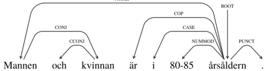
Mannen och kvinnan är i 80-85 årsåldern .
ROOT NSUBJ CONJ CCONJ COP CASE NUMMOD PUNCT
Figure 2.2: Dependencies of the sentence “Mannen och kvinnan är i 80-85 årsåldern.” (“The man and the woman are in their eighties.”)
In figure 2.2, each relation in a sentence is visualized by an arc from the governor to its dependent. The dependency notion on the arc entails the grammatical relation between the dependent and its governor [6]. In this example, “Mannen” is the first conjunct in the conjunction “Mannen och kvinnan” and is thus the governor of “kvinnan”. “Kvinnan” is the governor of the coordinating conjunction “och” that links the conjuncts together. “Mannen” is also the head word of the nominal subject of the clause. Its governor “årsåldern”, the root of the clause, is the complement of the copular verb “är”. The preposition “i” is a case-marking element, and is a dependent of the noun it is attached to, in this case “årsåldern”. “Årsåldern” also has a numeric modifier, “80-85”. Lastly, “årsåldern” is also the governor of the period. For information on additional grammatical relations, see Universal Dependencies2.
Word Embeddings
Word embeddings are learned representations of words in the form of vectors with numerical values. The fundamental idea behind word embeddings is the distributional hypothesis, meaning that words that are similar in meaning will occur in similar contexts [21]. The embedding vector can have hundreds of dimensions, where each dimension represents a latent feature that encodes different properties of a word [22]. Using this dense representation, the number of features will be much smaller than the size of the vocabulary, in contrast to if one would use for example the sparse vector representation one-hot encoding.
In this thesis, the word embeddings are obtained by using a pre-trained fastText model. The model was trained using Continuous Bag-of-Words (CBOW), which is a neural network that learns the embedding by predicting a word based on its context. Figure 2.3 shows the four closest surrounding words as input and the predicted word as output. For further information on the CBOW model, see [23].
Figure 2.3: CBOW training model from [23]
The fastText model learns representations for character n-grams and instead of assigning a distinct representation to each word, the words are represented as bags of n-grams. This method makes it possible to compute representations for words that are previously unseen to the model [24].
As the word embeddings are in the form of vectors with numerical values, it is possible to use them as a feature vector directly and avoid processing it further with manually engineered rules.
2.5 Evaluation Metrics
This section presents the definitions of the metrics that are used to evaluate the methods.
2.5.1 Precision
Precision is calculated as the number of correctly classified anaphor-antecedent pairs (true positives) divided by the number of pairs that were classified as anaphor-antecedent (true positives and false positives).
P recision = T P
T P + F P (2.25)
2.5.2 Recall
Recall is calculated as the number of correctly classified anaphor-antecedent pairs (true positives) divided by the number of pairs that according to the annotated dataset are correct anaphor-antecedent pairs (true positives and false negatives).
Recall = T P
T P + F N (2.26)
2.5.3 F1-score
F1-score is calculated as the harmonic mean of precision and recall. F1score = 2⇤
P recision⇤ Recall
Related Work
The subject of this thesis is pronoun resolution in Swedish. Due to limited research on Swedish pronoun resolution, this chapter will also cover research conducted in English, as well as research on coreference resolution.
3.1 Pronoun and Coreference Resolution in
Swedish
In 1988, Fraurud presented a simple algorithm for pronoun resolution which was evaluated on three different types of texts (stories, reports, and articles) in Swedish [25]. The algorithm consists of two parts, where the first part is finding all candidate antecedents of a pronoun based on a number of constraints. For instance, these constraints ensure that the candidate precedes the pronoun in the text and agrees with the pronoun in number, animacy, and gender. The second part is selecting an antecedent among the candidates. The most recent candidate will be selected as antecedent unless there is another candidate which is the subject of the same clause as the most recent candidate. If this is the case, and the pronoun is not a so-called semi-demonstrative (e.g. “denne”, “denna”), the subject candidate will be selected as antecedent. The input text presented to the algorithm had NPs, subject NPs, clauses, and sentences identified. In addition to this, the algorithm presupposes a lexicon with information on animacy and gender of nouns and pronouns to be able to determine agreement. Evaluated on all three types of texts, the correct antecedent was chosen 79.2% of the time. When excluding the cases where there was only one possible candidate, the correctness ratio decreased to 71.5%.
In 2010 Nilsson [7] presented a hybrid method to coreference resolution in Swedish, which combined a data-driven approach with linguistic knowledge. The linguistic knowledge is applied in the feature selection as well as in the selection of candidate antecedents. The data-driven method used to predict coreferent was Memory-Based Learning (MBL) [26], which is a supervised method based on storing experiences in memory and reusing solutions for solving new, similar problems. The knowledge-based method used for selecting candidates for anaphor-antecedent pairs is based on the Accessibility Theory of referring expressions [27]. This theory is focused on the relation between the referential form of a noun phrase and its cognitive status — its accessibility as an antecedent. The instance selection is based on determining how likely it is that an anaphor-antecedent pair is coreferent based on their degree of accessibility. This method was used to discard unlikely pairs before the step of the classifier labeling pairs as coreferent or not, in order to increase the performance of the classifier. In contrast to most other approaches to pronoun resolution, agreement between the anaphor and the candidate antecedent was not implemented as a hard constraint when detecting candidates, but rather as a feature during classification. This was to allow for coreference links between for example “regeringen” (“the government”) and “de” (“they”).
3.2 Pronoun and Coreference Resolution in
English
In 1976 Hobbs [11] suggested the Naive algorithm for finding the antecedents of third person pronouns, a method that searches a syntactic tree in a left-to-right, breadth-first order and applies certain requirements. The algorithm had a success rate of 82% when evaluated on 300 examples of pronouns from three different types of texts. The success rate was even higher when the algorithm was combined with selectional constraints (e.g. dates, places, and large fixed objects cannot move). However, there are sentences where it was impossible to find the correct antecedent without additional knowledge, for example when a sentence had ambiguous meaning. According to Hobbs, some examples could not be easily handled by the algorithm, but as their appearances were rare there was no gain in complicating the algorithm in order for it to handle these examples.
In 1994 Lappin and Leass [28] developed the algorithm RAP (Resolution of Anaphora Procedure) which determines the correct antecedent based on salience measures derived from syntactic structure. The salience measures are calculated by weighted factors, meaning that a candidate antecedent associated with factors of high weight is probably the correct antecedent. The factor’s weight reflects its relative importance. The two highest weighted factors are the following:
• If the candidate is in the same sentence as the referring expression. • If the candidate is the subject of the clause.
The algorithm has a high preference of intrasentential anaphora (the antecedent and reference occurs in the same sentence), which is indicated by the fact that the salience weight of an antecedent is halved each time a sentence boundary is crossed. This rather severe reduction in salience weight might make the algorithm choose an incorrect antecedent because of recency. In 1998, Mitkov suggested a knowledge-poor approach to resolving pronouns in technical manuals [29]. The approach is based on identifying a set of candidate antecedents, evaluating them by several heuristics, and assigning the candidates different scores depending on these heuristics. Finally, the candidate with the highest total score is considered most likely to be the antecedent of the pronoun in question. The heuristics, called antecedent indicators, give advantage to candidates that, for example, are frequently mentioned in the text and candidates that appear close to the anaphor. There are also penalizing heuristics, the algorithm will disfavor candidates that are indefinite or that are part of a prepositional phrase. Mitkov found that the approach struggled in finding the correct antecedent in sentences with too complicated syntax, and stated that it was a consequence of the system being knowledge-poor. Even so, the performed evaluation showed a success rate (calculated as precision over recall) of 89,7% when evaluated against the corpus of technical manuals.
In 2002, Mitkov further developed the method for anaphora resolution which resulted in the fully automated algorithm MARS [30]. The improved algorithm had some additions to the robust knowledge-poor approach, including a dependency parser as the main pre-processing tool and three additional antecedent indicators.
A detailed description of Mitkov’s method for pronoun resolution can be found in section 3.3.
In 2001 Soon et al. presented a learning approach to coreference resolution of noun phrases in unrestricted text that had performance comparable to the state-of-the-art non-learning systems of that time [8]. The supervised learning approach requires a small corpus of annotated training documents. To first determine all markables (anaphors and antecedents) of a text, a pipeline of NLP modules was used. Three major modules were a part-of-speech (POS) tagger, an NP identification module, and a named entity recognition (NER) module which are all based on Hidden Markov Models (HMM) [31]. The classifier was learned using C5, which is an updated version of the decision tree learning algorithm C4.5 [32]. The classifier is presented with a pair of markables and decides if they corefer based on a feature vector consisting of 12 features. The features derive information from both the anaphor and candidate antecedent, for example if either of them is a pronoun, if they agree in gender and number and if there is a string match between them. Some of the features are boolean and some are numerical, e.g. the distance feature which yields a number corresponding to the number of sentences between the markables.
In 2006, Yang et al [19] proposed a kernel-based method for pronoun resolution. By using a Support Vector Machine (SVM) along with a convolution tree kernel, they could automatically mine the knowledge embedded in parse trees, instead of having to limit the information to a number of manually engineered features. The main idea behind using a convolution tree kernel was to compare the substructures of trees to find out to what degree they contained similar information. The data instances were represented by a constituency parse tree containing the pronoun and the candidate antecedent, as well as the first level children of the nodes in between. When evaluated on three types of news texts (newswire, newspaper, and broadcast news) the kernel-based method performed significantly better than both the baseline using only manually designed features and the implementation of Hobbs’ Naive algorithm [11]. The highest success rate was obtained when using a composite kernel to combine the structured features and manually engineered features. The success rate was calculated as the ratio of the number of correctly resolved anaphors over the number of all anaphors. An anaphor was deemed correctly resolved if the anaphor and the selected antecedent belonged to the same coreference chain.
In 2017, Simova et al [33] explored the usefulness of features derived from word embeddings to resolve coreference. The features derived were embedding cluster and cosine similarity, as well as including the embedding vector directly. These were added as additional features to the baseline coreference system cort [34]. The highest F1-score was obtained when extending the standard features with a combination of all three embedding related features. However the improvement was very modest, 59.19% for the baseline compared to 59.72% with the additional features. The low improvement might implicate that the knowledge encoded by these features was more or less the same as the knowledge encoded in the manually engineered features of the baseline system.
3.3 Mitkov’s Algorithm
In this section, the steps of Mitkov’s algorithm are described. The steps are described as applied to one anaphoric reference in a text.
Initially, all NPs preceding the anaphoric reference in the current sentence and the two preceding sentences are collected. From these NPs, only the NPs that agree in gender and number (see agreement in section 2.2.2) with the anaphor will be kept as potential candidate antecedents. In the next phase, antecedent indicators are applied to each candidate and they are assigned a score (-1, 0, 1 or 2) for each indicator. Lastly, the scores are summed and the candidate with the highest aggregate score is proposed as antecedent of the anaphor in question. In the event of two candidates having an equal score, the candidate with the higher score of a certain indicator is favored. The order of importance of the decisive indicators is presented in the list below.
1. Immediate reference 2. Collocational pattern 3. Indicating verbs 4. Recency
Definiteness
Definite NPs will score 0 and indefinite NPs will be penalized by -1. This is due to the fact that definite NPs in earlier sentences are more likely antecedents of pronominal anaphors than indefinite ones.
Givenness
NPs in previous sentences that represent the given information in a text (the theme) will score 1 since they are deemed good candidate antecedents. Consequently, NPs not representing the given information will score 0. The theme is given by the first NP in a non-imperative sentence.
Indicating Verbs
There is a certain set of verbs for the English language that are viewed as particularly good indicators of the following NP to be an antecedent. Thus, the first NP following one of these verbs will score 1. The set is presented in full below.
Verb set = {discuss, present, illustrate, identify, summarise, examine, describe, define, show, check, develop, review, report, outline, consider, investigate, explore, assess, analyse, synthesise, study, survey, deal, cover} In Multilingual Anaphora Resolution (1999), Mitkov adapted the anaphora resolution algorithm to Polish. The corresponding verb set contained the equivalent verbs in Polish along with their synonyms [35].
Lexical Reiteration
Items that are repeated are likely to be a good candidate for antecedent. An NP that is repeated in the same paragraph at least twice will score 2, if it is repeated once it will score 1, and if there are no repetitions it will score 0. Lexically reiterated items include not only the exact NP but also synonymous NPs, and NPs with the same head.
Section Heading Preference
An NP occurring in the heading is considered the preferred candidate and will score 1.
“Non-prepositional” Noun Phrases
An NP that is non-prepositional is considered more likely to be an antecedent than a prepositional NP, thus a prepositional NP will be penalized with -1.
Collocation Pattern Preference
This indicator will favor the candidates having identical collocation patterns with a pronoun, which will score 2. Identical collocation means that the exact phrase will occur somewhere else in the same text, but with a pronoun instead of a noun phrase. The pattern that is considered is verb NP(or pronoun) and the corresponding NP(or pronoun) verb, where the verb is the same in both occurrences. Consider example (11).
(11) a. Advokaten ansökte redan 2013 om kontaktförbud. 2015 ansökte han på nytt om kontaktförbud.
b. (The lawyer applied for a restraining order in 2013. In 2015 he applied again for a new restraining order.)
Immediate Reference
The immediate reference is a modification of the collocation reference, and is a useful indicator for technical manuals, which is the text domain that this algorithm was originally developed for. This rather special case regards sentences of the form “...(You) V1 NP ... con (you) V2 it (con (you) V3 it)”, where con is part of the set containing the conjunctions “and”, “or”, “before”, and “after”. The NP following the first verb is considered a very likely candidate for antecedent of “it”. In this case, the NP will be assigned the maximum score of 2.
Referential Distance
Regarding complex sentences, NPs in the previous clause will score 2, NPs in the previous sentence will score 1, nouns that are two sentences back will score 0, and nouns three sentences back will be penalized by -1. In simple sentences, NPs in the previous sentence will score 1, NPs that are two sentences back will score 0, and nouns that are three sentences back will be penalized by -1. Thus, in complex sentences, the most probable candidate is situated in the previous clause. In simple sentences, it is most probably in the previous sentence. In both cases, candidates are penalized as the distance gets larger. How to determine if a sentence is complex or simple is not defined. For the
reimplementation, a sentence is considered to be complex when it contains more than one clause, see section 4.3.1.
Term Preference
NPs representing words in the field are considered more likely to be the antecedent than those that are not. NPs representing terms in the field will score 1.
3.4 MARS Additions to Mitkov’s Algorithm
MARS is developed from Mitkov’s algorithm, with some alterations [30]. This section presents the antecedent indicators that were added to the original indicators.
Boost Pronoun
Pronouns referring to an NP represent additional mentions of that entity and thus increase its topicality. If the actual antecedent is located more than two sentences prior to the anaphoric reference, the pronoun candidate is seen as a “stepping stone” between the anaphor and its more distant antecedent. Thus, pronoun candidates will score 1.
Syntactic Parallelism
An NP with the same syntactic role as the pronoun is likely to be the antecedent, thus it will score 1. The additional pre-processing in form of a dependency parser used by MARS provides the syntactic role of the NP.
Frequent Candidates
This heuristic is constructed from the observation that throughout an entire document, most pronouns refer to few entities. Consequently, the three NPs that occur most frequently in the set of candidate antecedents will score 1 point each.
Methods
This chapter presents the methods used in the heuristic-based and data-driven implementations of pronoun resolution, as well as the initial construction of the corpus.
4.1 Construction of the Corpus
This section contains a description of the steps in the pipeline of constructing the corpus. Figure 4.1 presents an overview of the major steps of the pipeline with the corresponding external tools in italics.
Scraping news articles Scrapy Annotation of articles Textinator Tokenization Granska POS-tagging, dependency parsing StanfordNLP Shallow parsing Granska Figure 4.1: Pipeline presenting the construction of the corpus
4.1.1 Web Scraping
The content for the dataset was gathered by continuously scraping Aftonbladet1 in November 2019. For this purpose, Scrapy2 was used, which is a Python framework for web scraping. The reason for choosing Aftonbladet was the frequent circulation of news articles as well as the wide range of articles that were not blocked by a paywall. The scraped articles were later
1https://www.aftonbladet.se/nyheter 2https://github.com/scrapy/scrapy
processed by removing duplicate articles and articles of a length too short to be useful.
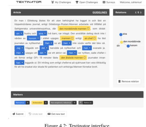
4.1.2 Annotation
After collecting articles, they were annotated using Textinator3(see figure 4.2). The annotation model that was used is link-based [12], meaning that each pronoun in the text is marked and connected to its antecedent. When searching for the antecedent the whole span of the current article was considered, and if there were several options as antecedent, the one that was closest to the anaphor was chosen. Each referring pronoun has only one antecedent, but that antecedent can be referred to by several different pronouns. If the pronoun had no antecedent present, or it was a cataphoric reference, the pronoun was marked as “not anaphoric reference”. If a plural pronoun had a conjunction as antecedent, the antecedent was annotated. However, if the pronoun had split antecedents, the pair was omitted. Furthermore, generic references and pleonastic pronouns (see section 2.3) were omitted as references.
Figure 4.2: Textinator interface
4.1.3 Text Pre-processing
Being able to use the corpus as input for the pronoun resolution algorithms required several steps of pre-processing of the text, which will be described in this section.
Tokenization
As two separate tools performing tokenization were used in the pipeline, StanfordNLP [36] and Granska Text Analyzer [37] (hereinafter referred to as Granska), the text was tokenized using Granska prior to the further processing using both systems. This was to avoid having the text tokenized in two different ways, which made the outputs difficult to merge at the end of the pipeline. One reason for using Granska was that it has internal rules for dealing with multi-word expressions that should be considered one word, such as “i dag” (“today”), “i sin tur” (“in turn”), and “bland annat” (“including”). Another reason for choosing Granska over StanfordNLP was that it overall performed more reasonable tokenization, in particular when the text contained non-alphabetic characters (see table 4.1).
Table 4.1: Different tokenizations using Granska and StanfordNLP
(a) Tokenization of the text “inte är några änglar”
Token index 0 1 2 3 4 5
Granska " inte är några änglar " StanfordNLP "inte är några änglar"
(b) Tokenization of the text “Låt oss utarbeta en bra deal!”
Token index 0 1 2 3 4 5 6 7 8
Granska " Låt oss utarbeta en bra deal ! " StanfordNLP " Låt oss utarbeta en bra deal!"
Part-of-Speech Tagging and Dependency Parsing
Part-of-Speech (POS) tagging was performed to identify the word class (noun, verb, etc) of each word in the text. The morphological features gender (uter/neuter) and number (singular/plural) were generated as well. Dependency parsing was performed to get the governor of each word, and
the dependency relation the word has to its governor. The StanfordNLP POSProcessor and DepparseProcessor trained on the Swedish corpus Talbanken were used for this purpose [36].
Shallow Parsing
As the antecedent indicators in Mitkov’s algorithm are highly dependent on NPs, identification of syntactic phrases was required. The identification of phrases was performed using Granska, which is a rule-based shallow parser [37].
Determining the Head of a Noun Phrase
In noun phrases consisting of several nouns, the last one was selected as head noun, unless the noun phrase contained a relative clause, then the first noun was chosen as the head noun.
Determining Gender and Number of a Noun Phrase
The gender and number were usually decided from the morphological features of the head of the noun phrase. In some cases, this method would give the wrong information, for example when the noun phrase contained a conjunction. To correct this, the number was set to plural when the noun phrase contained the conjunction “och” (“and”).
Manual Corrections of Erroneous Morphological Features
Using StanfordNLP, the personal pronoun “ni” was consistently given the number attribute singular, when in fact it should be plural. This was manually corrected during the text pre-processing.
Omitting Pronouns as Possible Candidate Antecedents
A number of Swedish pronouns can act as the head of a noun phrase. During the annotation, the chosen antecedent of anaphoric references was always a non-pronominal NP. The reason for not choosing pronouns is the lack of information that a sole pronoun carries. If there is a chain of pronouns between the original antecedent and the current pronoun, one would still have to look for the original non-pronoun antecedent to understand what the current pronoun is referring to. Not omitting the candidates consisting of only pronouns would possibly give misleading results, as determining a pronoun to be the
most probable antecedent would never be the correct answer according to the annotated data.
Ambiguity in Determining Word Class of “den” and “det”
As presented in 2.3, “den” and “det” can be used both as a pronoun (“it”) and as a determiner (“the”). The word class ambiguity occasionally caused a situation where a word was annotated as a pronoun but classified as a determiner during POS-tagging. In this case, the word would erroneously be considered as not an anaphoric reference. This was manually corrected by setting the word class to pronoun instead of determiner, in the case that the word had been annotated as a pronoun.
4.2 Selecting the Candidate Antecedents
For the heuristic method and the data-driven method, the sets of candidate antecedents were selected using the same method. A set of potential candidates was identified for each anaphoric pronoun in a text. Initially, all noun phrases before the anaphor in the same sentence and the two prior sentences were considered to be candidates. From this set, the candidates that did not agree in gender and number were discarded. A positive instance was created with the anaphor and the annotated antecedent, and negative instances were formed with the anaphor and each of the remaining candidates.
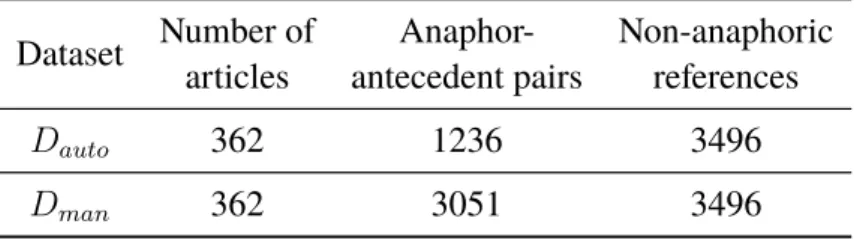
Occasionally, the annotated antecedent was not part of the identified candidates, which will be further discussed in section 6.3. Due to the inability to detect all the annotated antecedents, two datasets were created. The first dataset, Dauto, contains all anaphoric references with its corresponding antecedents that were detected using the method described above. The second dataset, Dman, is an extension of Dauto with the addition that all annotated antecedents are manually added in the case that it was either undetected or discarded using the method described.
4.3 Heuristic Approach
The reimplementation of Mitkov’s algorithm was run on the entire dataset. For each anaphoric pronoun in the text, the candidate antecedents were collected using the method described in section 4.2. After collecting the set of
candidates, each candidate was scored according to the antecedent indicators (further described in section 4.3.2). Lastly, the scores were summed, and the candidate with the highest aggregate score was chosen as the antecedent.
4.3.1 Modifications of Mitkov’s Algorithm
Some adjustments to the pronoun resolution algorithm described in section 3.3 had to be made. This is due to that in this thesis the algorithm was applied to texts of a different language and genre than what it was originally developed for. Additionally, some indicators were not applicable due to the limited information about the corpus.
As presented in 3.3, in the case of several candidate antecedents having an equal aggregated score, there is an order of importance of the decisive indicators. This order was altered since one of the decisive indicators was omitted in this version of the algorithm. The altered order of importance is presented in the list below.
1. Collocational pattern 2. Indicating verbs 3. Recency
4.3.2 Reimplemented Antecedent Indicators
This section presents the antecedent indicators that were applicable in this implementation, along with a presentation of possible adjustments that have been made.
Definiteness
This antecedent indicator was implemented without adjustments.
Givenness
Indicating Verbs
As presented in 3.3, the verb set was translated to Polish when adapting the algorithm on texts in Polish, which is why the verb set was translated to Swedish in this adaption for texts in Swedish.
Lexical Reiteration
Because of the lack of tools to identify synonymous NPs, the reimplementation of this indicator only took the exact NP into account. In practice, all NPs were mapped to the number of occurrences in the text. The entire text was considered, in contrast to the current paragraph as in the original version, due to the difficulty in determining paragraphs.
“Non-prepositional” Noun Phrases
This antecedent indicator was implemented without adjustments.
Collocation Pattern Preference
This antecedent indicator was implemented without adjustments.
Referential Distance
This antecedent indicator scores candidates differently based on if the sentence is complex or simple. As a method for determining the complexity was not disclosed, a sentence was here considered to be complex if it contained more than one clause, and simple otherwise.
4.3.3 Omitted Antecedent Indicators
This section presents the omitted antecedent indicators along with an explanation for omitting them.
Section Heading Preference
This indicator was omitted due to the nature of the used corpus. While news articles usually have a heading (the title), it is not necessarily a definition of the domain of the following text, as it is in technical manuals. For news articles, especially the nature of the specific newspaper used for the corpus of this thesis, the purpose of the heading is rather to evoke the readers’ interest than to classify the information of the article.
Immediate Reference
This indicator is quite specific for technical manuals, capturing a written instruction. It will probably not have the same applicability in different genres of text, which is why the indicator was omitted.
Term Preference
This indicator was omitted due to the lack of tools to determine if a word or phrase is in the field.
4.4 Data-driven Approach
The data-driven approach to pronoun resolution is using an SVM (see section 2.4) to perform a binary classification — given a pair consisting of an anaphoric reference and a candidate antecedent, the SVM model determines if the candidate is the correct antecedent (labeled as 1) or not (labeled as -1). A pair was constructed from an anaphoric reference with each of its candidate antecedents, which were selected using the method described in section 4.2. As there can be only one positive instance (the correct antecedent), but possibly several negative instances (all other candidates), this naturally leads to an imbalanced dataset. The method for rebalancing the dataset is explained in section 4.4.3.
In contrast to the heuristic method, the data-driven method classified each data sample (pair of anaphor and candidate) independently of the other candidates associated with the anaphor. This is because the candidates associated with an anaphor were not presented as a set where only one candidate could be the correct one, but rather as part of the entire dataset where each pair was one labeled data sample.
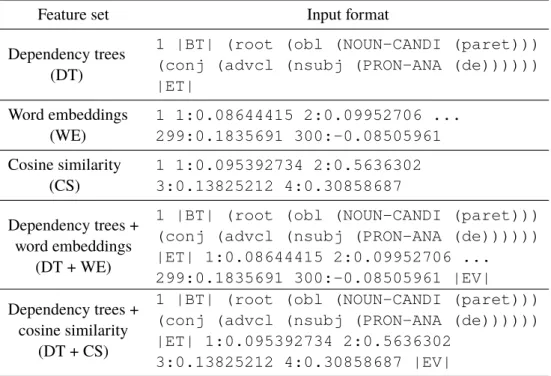
The data samples had different formats depending on what kernels and features were used. When using dependency trees as a feature, a data sample was represented as a tree in string format. A dependency tree was constructed for the entire article in which the sample originates, and was then pruned to contain only the shortest path between the candidate and the anaphor (further explained in section 4.4.2). As the kernel function determines the similarity between two trees using numerical vectors, the dependency tree is ultimately represented as an implicit numerical vector (see section 2.4.2), where each
position i corresponds to the number of times tree fragment i occurred in the considered tree. The dimension of this vector is the total number of unique tree fragments present in the dataset. When using kernels (see section 2.4.2), there is no need to explicitly construct these high-dimensional vectors, as the kernel function defines the inner product of two vectors in the transformed space.
When using word embeddings as a feature, as well as the cosine similarity between them, the generated vectors were numerical in their original form and did not demand further processing. See section 4.4.2 for further information on how word embeddings were used.
The different features were used with different kernel functions, which are presented in section 4.4.1. Lastly, in section 4.4.4, a detailed description of the used SVM implementation is presented.
4.4.1 Kernels
When using only the dependency trees feature, a Partial Tree Kernel was used. For the word embeddings feature and the cosine similarity feature, a polynomial kernel and an RBF-kernel were used respectively. See section 2.4.2 for more information about the kernels.
In order to combine the features, two different composite kernels were used, which are presented in equation 4.1 and equation 4.2,
Ks(o1, o2) = Kt(T1, T2) + Kp(v1, v2) (4.1) Ks(o1, o2) = Kt(T1, T2) + KRBF(v1, v2) (4.2) where Ktis a Partial Tree Kernel, Kpis a polynomial kernel, and KRBF is an RBF kernel. Tiis the tree representation and vi is the vector representation of the data instance oi.
4.4.2 Features
The feature vectors used with the SVM model were constructed from dependency trees and word embeddings, which are further described in this section.
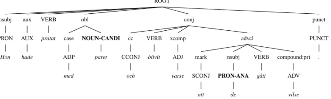
Dependency Trees
The dependency relations in a tree are usually presented as labeled edges, as in figure 4.3. As the model cannot interpret labeled edges, the provided dependency relations as well as the corresponding POS-tags need to be converted to nodes like the lexicals. To address this, a Grammatical Role Centered Tree (GRCT) structure [38] was used.
Hon hade pratat med paret och blivit varse att de gått vilse . PRON AUX VERB ADP NOUN CCONJ VERB ADJ SCONJ PRON VERB ADV .
root nsubj aux obl case conj cc xcomp advcl mark nsubj compound:prt punct
Figure 4.3: Dependency tree with relations on arcs
A GRCT structure is presented in figure 4.4, where the parsed sentence is the same as in figure 4.3. The GRCTs were constructed such that the dependency relation node is the parent of the word class node, which in turn is the parent of their associated lexical. The word class nodes of the anaphor-candidate pair are explicitly marked with “CANDI” and “ANA” respectively. The anaphor always consists of exactly one word, but the candidate can contain several words. In the case of a multi-word candidate, the corresponding word class node of all words are marked with “CANDI”.
ROOT nsubj PRON Hon aux AUX hade VERB pratat obl case ADP med NOUN-CANDI paret conj cc CCONJ och VERB blivit xcomp ADJ varse advcl mark SCONJ att nsubj PRON-ANA de VERB gått compound:prt ADV vilse punct PUNCT .
Figure 4.4: GRCT with labeled anaphor and candidate
A GRCT was constructed for the entire text in an annotated article and not for individual sentences, as the anaphor and the candidate can appear in different sentences. To construct a tree for an entire text, a tree was generated for each sentence and was attached to an upper pseudonode. To avoid excess
information, only the shortest path between the anaphor and the candidate antecedent was given as input to the model, as in figure 4.5, which is a substructure of the tree in figure 4.4.
ROOT obl NOUN-CANDI paret conj advcl nsubj PRON-ANA de
Figure 4.5: The final GRCT substructure
Word Embeddings
The word embeddings were obtained by a pre-trained fastText model (see section 2.4.3). The dimension of the word embeddings were 300, and the model was trained on texts from Wikipedia as well as Common Crawl. The features derived from word embeddings are the embedding vector for the candidate antecedent (its head4) in its original form, as well as a combination of several cosine similarity measures.
Four cosine similarities were used, as in [33], and were computed as in equation 4.3. The cosine similarity was computed between the embedding vectors of the anaphor and the head word of the candidate antecedent (ANA, ANTE), between the governor of the anaphor and the governor of the candidate antecedent (GOVAN A, GOVAN T E), as well as (ANA, GOVAN T E) and (ANTE, GOVAN A). cos( ~v1, ~v2) = ~ v1· ~v2 ||~v1|| ||~v2|| (4.3) The idea behind using the word embedding vector as a feature was that the vector can provide information about the different semantic features of a word, which might be useful when resolving pronouns. The idea behind using cosine similarity as a feature was that a correct candidate antecedent should be more similar to the anaphor than an incorrect candidate.

![Figure 2.3: CBOW training model from [23]](https://thumb-eu.123doks.com/thumbv2/5dokorg/4981425.136991/28.892.294.540.326.602/figure-cbow-training-model-from.webp)