Analysis of global debris-flow fatalities and related socioeconomic factors from 1950 to 2011, An

AN ANALYSIS OF GLOBAL DEBRIS-FLOW FATALITIES AND RELATED SOCIOECONOMIC FACTORS

FROM 1950 TO 2011

by

A thesis submitted to the Faculty and the Board of Trustees of the Colorado School of Mines in partial fulfillment of the requirements for the degree of Master of Science (Geological Engineering). Golden, Colorado Date Signed: Casey Dowling Signed: Dr. Paul M. Santi Thesis Advisor Golden, Colorado Date Signed: Dr. John D. Humphrey Professor and Head Department of Geology and Geological Engineering

ABSTRACT

Debris flows cause significant damage and fatalities throughout the world. However, some debris flows only take a few victims, while others kill hundreds, and the differences between these events is not well understood. This study addresses the overall impacts of debris flows on a global scale from 1950 to 2011. Two hundred thirteen events with 77,779 fatalities were recorded from academic publications, newspapers, and personal correspondence. Spatial, temporal, and physical characteristics were documented and evaluated. In addition, multiple socioeconomic indicators were reviewed and statistically analyzed to evaluate if vulnerable populations are disproportionately affected by debris flows. This research provides evidence that populations with lower social, political, or economical standing are more at risk for debris–flow related fatality. Specifically, higher levels of fatalities tend to occur in developing countries, characterized by less wealth, more corrupt governments, and weaker healthcare systems. The median number of deaths per flow in developing countries is 23, but only 6 in advanced

countries. The analysis also indicates that debris flow occurrence and deadliness is affected by seasonal precipitation patterns, as the most common trigger for fatal events has been found to be extreme precipitation, particularly in the form of large seasonal events like cyclones and

monsoon storms. Rainfall caused or triggered 144 of the 213 fatal debris flows within the database. However, it is the more uncommon and catastrophic triggers, such as earthquakes, and landslide dam bursts that tend to create more deadly debris flows, with a median fatality count greater than 500 while rainfall induced debris flows have a median fatality rate of only 9 per event.

TABLE OF CONTENTS

ABSTRACT ... iii

LIST OF FIGURES ... vii

LIST OF TABLES ... xi

ACKNOWLEDGEMENTS ... xii

CHAPTER 1 INTRODUCTION ... 1

CHAPTER 2 PRIOR RESEARCH ... 3

CHAPTER 3 METHODOLOGY ... 7

3.1 Debris Flow Event Collection ... 7

3.2 Data Analysis ... 11 3.2.1 Descriptive Statistics ... 11 3.2.2 Spatial Analysis ... 12 3.2.3 Temporal Analysis ... 13 3.2.4 Physical Characteristics ... 14 3.2.5 Socioeconomic Analysis ... 16 3.2.6 Regression Analysis ... 17 CHAPTER 4 RESULTS ... 19 4.1 Descriptive Statistics ... 19 4.2 Spatial Results ... 20 4.3 Temporal Results... 20 4.3.1 Database Overview ... 23

4.3.2 Monthly Analysis ... 25

4.4 Physical Attribute Results ... 30

4.4.1 Warning Signs ... 30

4.4.2 Mitigation ... 31

4.4.3 Triggers and Causes ... 32

4.4.4 Debris-Flow Volume ... 34

4.5 Socioeconomic Results ... 35

4.5.1 GDP per Capita Regression ... 36

4.5.2 Hospital Beds per Capita Regression ... 37

4.5.3 Maternal Mortality Rate Regression ... 39

4.5.4 Life Expectancy Regression ... 40

4.5.5 Corruption Perception Index Regression ... 42

4.5.6 Technical Journal Publications per Capita Regression ... 43

4.5.7 International Monetary Fund Classification ... 45

CHAPTER 5 DISCUSSION ... 47

5.1 Descriptive Statistics ... 47

5.2 Spatial Distribution of Fatal Debris Flows ... 48

5.3 Temporal Analysis of Fatal Debris Flows... 49

5.3.1 Database Overview ... 49

5.3.2 Monthly Analysis ... 51

5.4 Physical Characteristics of Fatal Debris Flows ... 55

5.4.1 Warning Signs ... 55

5.4.3 Triggers and Causes ... 56

5.4.4 Debris-Flow Volume ... 57

5.5 Socioeconomic Indicators ... 59

5.5.1 GDP per Capita Regression ... 59

5.5.2 Hospital Beds per Capita Regression ... 59

5.5.3 Maternal Mortality Rate Regression ... 60

5.5.4 Life Expectancy Regression ... 60

5.5.5 Government Corruption Regression ... 61

5.5.6 Technical Publications per Capita Regression ... 61

5.5.7 Socioeconomic Indicator Ranking ... 62

5.5.8 International Monetary Fund Classification ... 63

CHAPTER 6 CONCLUSIONS ... 65

REFERENCES ... 67

LIST OF FIGURES

Figure 4.1: Histogram of fatalities per debris flow recorded in the database. ... 20 Figure 4.2: Map showing distribution of recorded fatal debris flow within countries in the

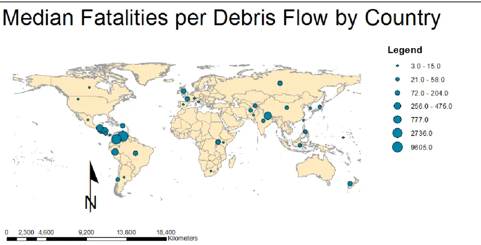
database. Dot size represents the number of fatal debris flows per country. ... 21 Figure 4.3: Map showing distribution of median debris-flow fatalities within countries

recorded in the database. Dot size represents the mean debris-flow fatalities per event in each country. ... 22 Figure 4.4: Bar graph showing the number of recorded fatal debris flows in the database by

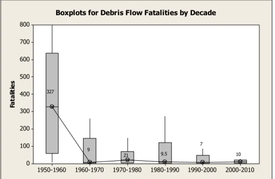
decade. ... 23 Figure 4.5: Boxplot of fatalities per debris flow by decade. The median value and its trend

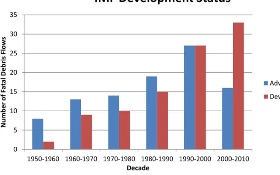
line are displayed. ... 23 Figure 4.6: Bar graph showing the number of recorded debris flows per decade subdivided by IMF development status. ... 24 Figure 4.7: Boxplot of fatalities per debris flow in advanced nations divided by decades. The

median value and its trend line are displayed. ... 24 Figure 4.8: Boxplot of fatalities per debris flow in developing nations divided by decades.

The median value and its trend line are displayed. ... 25 Figure 4.9: A.) Number of fatal debris flow per month for the database. B.) Mean fatalities

per debris flow by month for the database. ... 26 Figure 4.10: A.) Number of fatal debris flow per month in North America. B.) Average

fatalities per debris flow by month in North America. ... 26 Figure 4.11: A.) Number of fatal debris flow per month in Central America. B.) Average

fatalities per debris flow by month in Central America. ... 26 Figure 4.12: A.) Number of fatal debris flow per month in South America. B.) Average

fatalities per debris flow by month in South America. ... 27 Figure 4.13: A.) Number of fatal debris flow per month in Europe. B.) Average fatalities per

Figure 4.14: A.) Number of fatal debris flow per month in Africa. B.) Average fatalities per debris flow by month in Africa. ... 28 Figure 4.15: A.) Number of fatal debris flow per month in Asia. B.) Average fatalities per

debris flow by month in Asia. ... 28 Figure 4.16: A.) Number of fatal debris flow per month in Southeast Asia. B.) Average

fatalities per debris flow by month in Southeast Asia. ... 29 Figure 4.17: A.) Number of fatal debris flow per month in Oceania. B.) Average fatalities per debris flow by month in Oceania. ... 29 Figure 4.18: Graph of the long term warning signs for debris flows in the locations of fatal

debris flows. These values reflect the long term warning signs reported and do not necessarily represent the true frequency of warning signs, which are often omitted from news and literature reports. Categories are not mutually exclusive. ... 30 Figure 4.19: Graph of the short term warning signs for debris flows in the locations of fatal

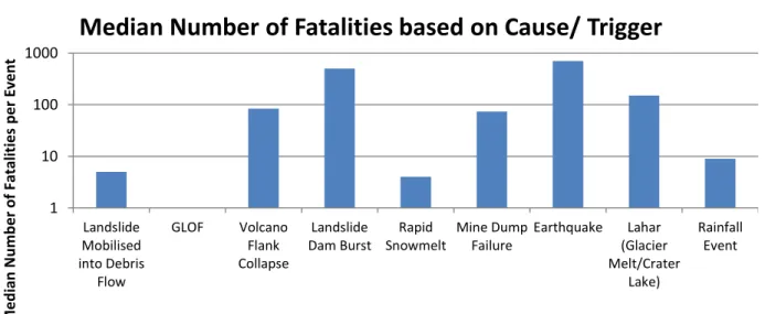
debris flows. These values reflect the short term warning signs reported and do not necessarily represent the true frequency of warning signs, which are often omitted from news and literature reports. Categories are not mutually exclusive. ... 31 Figure 4.20: Graph of debris-flow mitigation present in the locations of fatal debris flows. ... 31 Figure 4.21: Graph of the number of fatal debris flows by the cause/trigger. ... 32 Figure 4.22: Graph of the median number of fatalities per debris flow by cause/trigger. ... 32 Figure 4.23: Graph of the number of fatal debris flows triggered/caused by rainfall induced

events. ... 33 Figure 4.24: Graph of the median number of debris-flow fatalities by rainfall induced

cause/trigger. ... 33 Figure 4.25: Graph of number of fatalities depending on volume. The regression equation,

trend line with confidence and prediction intervals, as well as the R2 value are provided. ... 34 Figure 4.26: Residual versus fits plot for fatalities versus volume regression. ... 35

Figure 4.27: Line graphs of debris-flow fatalities depending on volume based on the

population. The R2 values and the regression found by Minitab are provided in the key for each population size. ... 35 Figure 4.28: Graph of the relationship between fatalities per debris flow and GDP per capita.

The P value, trend line with confidence and prediction intervals, as well as the R2 value are provided. ... 36 Figure 4.29: Residual versus fits plot for fatalities versus GDP per capita regression. ... 37 Figure 4.30: Graph of the relationship between fatalities per debris flow and the number of

hospital beds per capita. The P value, trend line with confidence and prediction intervals, as well as the R2 value are provided. ... 38 Figure 4.31: Residual versus fits plot for fatalities versus hospital beds per capita regression. 38 Figure 4.32: Graph of the relationship between fatalities per debris flow and MMR. The P

value, trend line with confidence and prediction intervals, as well as the R2 value are provided. ... 39 Figure 4.33: Residual versus fits plot for fatalities versus MMR regression. ... 40 Figure 4.34: Graph of the relationship between fatalities per debris flow and life expectancy at birth. The P value, trend line with confidence and prediction intervals, as well as the R2 value are provided. ... 41 Figure 4.35: Residual versus fits plot for fatalities versus life expectancy at birth regression. 41 Figure 4.36: Graph of the relationship between fatalities per debris flow and CPI. The P value,

trend line with confidence and prediction intervals, as well as the R2 value are provided. ... 42 Figure 4.37: Residual versus fits plot for fatalities versus CPI regression. ... 43 Figure 4.38: Graph of relationship between technical journal publications per capita and

fatalities per event. The P value, trend line with confidence and prediction

intervals, as well as the R2 value are provided. ... 44 Figure 4.39: Residual versus fits plot for fatalities and technical journal publications per capita regression. ... 44 Figure 4.40: Histograms of fatalities per debris flows for developing and advance countries

Figure 4.41: Chart of the percentage of fatal debris flows in the database based on IMF

development status. ... 46 Figure 4.42: Chart of the percentage of fatalities in the database based on IMF development

LIST OF TABLES

Table 3.1: Information recorded in the Debris Flow Fatality Database. ... 8

Table 3.2: Population Classes ... 16

Table 4.1: Descriptive Statistics for the Debris Flow Fatality Database ... 19

Table 4.2: Volume Regression F Test Results ... 34

Table 4.3: Gross Domestic Product per Capita Regression F Test Results ... 36

Table 4.4: Hospital Beds per Capita Regression F Test Results ... 37

Table 4.5: Maternal Mortality Rate Regression F Test Results ... 39

Table 4.6: Life Expectancy Regression F Test Results... 40

Table 4.7: Corruption Perception Index Regression F Test Results ... 42

Table 4.8: Technical Journal Publication per Capita Regression F Test Results ... 43

Table 4.9: Descriptive Statistics for Advanced and Developing countries based on IMF Classification... 45

ACKNOWLEDGEMENTS

My sincere thanks goes to my advisor, Dr. Paul M. Santi, for providing the initial data for this research and guidance throughout its duration. I would also like to thank my committee members, Dr. Jerry D. Higgins and Dr. Wendy Zhou, for providing technical guidance. In addition, I would like to thank Dr. David N. Petley of the Landslide Blog, the Association of Engineering and Environmental Geologists, and the Geological Society of America for soliciting professionals to provide information on debris flow events. Finally, I would like to thank all those who provided information used in this research.

CHAPTER 1 INTRODUCTION

Debris flows are a common hazard in mountainous regions around the world. They have long been considered a particularly devastating geologic hazard due to their rapid velocities and ability to travel great distances. Debris flows are responsible for some of the largest landslide disasters in modern times (Jakob and Hungr, 2005), capable of burying entire cities and killing tens of thousands in a single event. While these large events are especially destructive, the cumulative effects of smaller debris flows over a wet season also can cause significant losses. Furthermore, population growth has driven development farther into debris-flow prone areas, causing increased risk from this hazard (Jakob and Hungr, 2005).

As geoscientists have become increasingly aware of the risk of debris flows, a large amount of research has been conducted to better understand the hazard. Many of these studies have focused on the physical characteristics and processes of debris flows. These include geologic settings, triggering mechanisms, transport processes, deposition characteristics and mitigation options. However across the research, there is a key piece of analysis missing. Presently, there are no publications which directly compile and analyze the losses of human life caused by debris flows.

Disregarding particularly devastating incidents, (e.g., Venezuela 1999, Taiwan 1996) debris-flow fatalities often have been lumped into the death tolls of large scale regional disasters such as earthquakes, volcanic eruptions, and hurricanes (Santi et al., 2010). This occurs because

debris flows often are a secondary process of these larger calamities (Jakob and Hungr, 2005). This practice undermines recognition of the impact of debris flows related to these events. While triggered by the overall disaster, damage from debris flows differs from that caused by flooding or extreme ground shaking and may be unexpected. If authorities are not aware of the potential impact of debris flows, funds for prevention or hazard response may be wrongly allocated; allowing debris flows to significantly increase the overall death toll (Santi et al. 2010). As Santi and others (2010) indicate, regional disasters cannot be prevented, but to some degree debris-flow hazards can be mitigated.

In addition to increased fatalities, it is also becoming evident that debris flows

disproportionally affect those with social disadvantages. A “disaster of social vulnerability” as defined by Hewitt (1997) is one which has particularly devastating effects on populations with resource limitations, such as economic, space, and influence/power constraints. The perception of debris flows as a “disaster of social vulnerability” has been alluded to in recent publications (Santi et al. 2010), but has not been supported by quantitative data.

This thesis provides a debris-flow fatality database to address the above needs within the field of debris-flow research. It provides quantitative data to evaluate certain physical and

socioeconomic indicators, which may be indicative of a location’s risk to fatal debris flows. This evaluation tests the hypothesis that debris flows are in fact “disasters of social vulnerability.” Finally, by providing quantitative data on debris-flow fatalities, the database can be used to validate further research on debris flows such as effectiveness of debris-flow warning systems and mitigation techniques.

CHAPTER 2 PRIOR RESEARCH

Substantial amounts of research have been performed in the field of landslides, with increasing focus on debris flows in recent years. As researchers have delved into the physical mechanics of debris flows, significant human losses across the globe have been attributed to the phenomenon. However, this understanding is often over-generalized, with no specific details or quantitative information. Jakob and Hungr’s introduction to their compilation on debris-flow hazards (Jakob and Hungr, 2005) recognizes the need for more specific data and states “direct debris flow damage…is difficult to quantify.” Many large debris flow disasters have been studied in great detail (e.g., Garcia-Martinez and Lopez, 2005; Jan and Chen, 2005; Sanchez et al., 2009) and some publications contain inventories of events for particularly famous locales (Guadagno and Revellino, 2005; Kanji et al., 2003), or for the broader topic of landslide fatalities (Petley et al., 2005), but there is currently no global database specific to debris flows.

The first attempt at a quantitative loss database for the all-encompassing hazard of landslides is that of Petley and others (2005). It was found that while some local and national databases had been created, there was no global landslide loss database. Prior to this study, landslide loss figures tended to be over-generalized, making it difficult to illustrate just how destructive landslides could be (Petley et al., 2005). In September of 2003, Petley and others began compiling a database of landslide incidents on a global scale. In the database, landslides are defined as “all soil/rock failures, including slides, flows and falls” (Petley et al., 2005). Debris flows were included only when they could be “clearly differentiated from a flood” (Petley

et al., 2005). Within the database, only landslides that caused fatalities were recorded, because fatalities are a universal currency with an identical value around the globe. Petley and others note that fatalities are the worst case scenario, representing the greatest loss occurring from a landslide, and they are one of the few things reliably reported around the globe no matter the level of development or remoteness of a setting. Data was gathered from a variety of sources including professional papers, media articles, government data, and aid agency reports (Petley et al., 2005).

Petley (2012) examined the trends in landslide fatalities from the landslide database covering the period between January 1, 2004 and December 31, 2010, excluding seismically triggered events. From this subset, he showed that locations of landslide fatalities were clustered in particular locations across the globe. Typically these locations had a combination of four characteristics: high relief, high rates of tectonic processes, intense precipitation, and dense human populations. He observed that, in general, regions with substantial amounts of research such as Italy and Hong Kong, had far fewer fatalities than those with limited landslide research. This occurred even though all four previously mentioned conditions existed. Japan was an exception; even though the country had intense research and mitigation, many landslides still caused fatalities. Petley (2012) found that the top fifteen countries with the most landslide fatalities during the period between 2004 and 2010 were all developing nations, supporting the hypothesis that landslides may disproportionately affect vulnerable populations.

While Petley’s (2012) research focused on landslides of all types, similar trends for debris flow fatality data collected in the database for this research are expected. This project differs from the work of Petley and others (2005) and Petley (2012) as it focuses only on debris flows and reviews data over a much longer period of time. This study also performs a statistical

analysis to identify trends between specific socioeconomic indicators and the severity of debris-flow impacts.

Jakob and others (2011) was one of the first quantitative risk assessments of debris-flow losses, based on building damage from 68 incidents around the world. They used a quantitative risk assessment to calculate the risk to a population from a hazard based on the probability of an event, the spatial and temporal probability, vulnerability, and the number of people at risk. Since the study was focused on the vulnerability of structures, a database was created to record the damage done to buildings from debris flows of varying sizes, depths, and velocities. Fatalities caused by the events were not recorded.

Rather than structural damage, the work of Santi and others (2010) focused on the socioeconomic factors which may influence the number of fatalities caused by debris flows. Santi and others (2010) is the first publication to suggest that debris flows are “disasters of social vulnerability,” in the same way that Hewitt (1997) describes earthquakes. These types of

disasters preferentially cause more fatalities in populations with various resource limitations, such as economic, space, and influence/power restrictions. Economic and space restrictions force these vulnerable populations to live in high hazard areas where the risk for debris flows is great and the topography may confine the population in times of disaster (Santi et al., 2010). Political power limitations prevent these populations from receiving the resources necessary to address the risk of debris flows (Santi et al., 2010). The paper included six case studies of fatal debris flows from around the world in which socioeconomic restrictions played a major role. Qualitative information from the case studies showed the victims were typically found to be living in high hazard areas, with no place to evacuate in the short time following the initiation of the debris flow (Santi et al., 2010). The authors speculate socioeconomic indicators may be

useful in measuring the vulnerability of populations; however, no quantitative measures were made for the six case studies.

CHAPTER 3 METHODOLOGY

This thesis aims to examine debris flow losses through the creation and analysis of a fatality database. To accomplish this task, fatal debris flow events were found through a variety of different sources with different levels of technical expertise. This involved differentiating debris flows from flooding and other forms of landslides. Furthermore, statistical analysis has been performed on the data to evaluate physical and socioeconomic trends common amongst fatal debris flows.

3.1 Debris Flow Event Collection

Over two hundred fatal debris flows have been recorded between the years 1950 and 2011. The term “debris flow” includes both debris and earth flows as defined by Cruden and Varnes (1996). This leads to the inclusion of flow-type failures which are both predominantly coarse-grained (debris) and predominantly fine-grained (earth) (Varnes, 1978). The volcanic counterpart of debris flows, lahars, have also been included in the database as these events cause similar damage to debris flows and fit the definition of debris and earth flows under Varnes’ (1978) classification. The database does not include flood fatalities. For each event, the database contains information on a variety of factors which address both the physical and socioeconomic conditions that may influence the number of fatalities caused by a debris flow. Information recorded in the database is provided in Table 3.1.

Table 3.1: Information recorded in the Debris Flow Fatality Database.

Topic Item

Spatial/ temporal information Country, location, date, time of day Flow information and effects Volume, number of fatalities

Short term warning High rainfall, local debris flows within 1-2 days, earthquake, hurricane rainfall, monsoon rainfall, wildfire within last 3 years, shaking of ground, roaring noises, observation of

landslide

Long term warning Recent history of debris flows, annual debris flows in region, prehistoric debris flow deposits, construction of debris flow mitigation, debris flow landforms, massive boulders on adjacent land

Cause/ trigger Landslide mobilization, glacial lake outburst flood, volcano flank collapse, landslide dam burst, glacial melt lahar, earthquake, rainfall (tropical cyclone rainfall, monsoon rainfall, winter storm rainfall, summer storm rainfall, rain following fire, rain on ash lahar, rain after land clearing, rain on snow)

Mitigation None, check dam, sabo dam, debris fence,

debris basin, deflection walls

Economic indicators Technical journal articles per capita (research investment surrogate), gross domestic product (GDP) per capita (indicator of economic development and wealth for country)

Healthcare indicators Maternal mortality rate (MMR) (indicator of development of a country’s healthcare system), number of hospital beds per capita (indicator of a country’s ability to provide emergency services), life expectancy at birth (indicator of development of a country’s healthcare system) Political indicators Government corruption index (GCI) (indicator

of a government’s ability to respond to emergencies)

Information for the database has been collected from a variety of published resources including: technical literature, newspaper articles, government documents, and aid organization filings. Technical literature was found online, through academic resources, and in library

records. Journalism sources were found online, in newspapers, and through journalism databases. Government and international aid documents were obtained through respective government, World Bank, and United Nations websites.

While technical literature correctly classified the type of slope movement, incorrect terminology often appeared in non-technical literature such as news media, government, and international aid documents. When an event was not classified specifically as a debris flow, the following system was utilized to evaluate whether the event belonged in the database. The terms “landslide” or “mudslide” are common phrases used when describing debris-flow events in non-technical articles. If only the term “landslide” was provided, article photographs were used to classify the type of slope movement, where evidence of flow movement indicated debris flows. If no photographs were available, the article’s description of the event was utilized. If keywords such as “flow” or “torrent” were used in the article, the event was recorded in the database, as these terms are indicative of the type of movement associated with debris flows. The term “mudslide” also alludes to rapid flow type behavior, but is often used for both earth and debris flow type slope movements in nontechnical sources. As it was not physically possible to

evaluate grain size distribution and make a proper classification, it was reasonable in the scope of this study to include both earth and debris flows in the database, thus allowing events termed as “mudslides” to be included. Debris flows were separated from floods by reviewing the

mechanisms of death. Death by burial or trauma from debris was assumed to be a debris-flow fatality while death from drowning was assumed to be caused by flooding.

Non-technical sources also tend to lump debris-flow fatalities with other fatalities occurring during regional disasters such as flooding from heavy rain or structural damage from earthquakes. The lumped number provided in these counts was not used in the database, as the

fatality count would have been inflated from deaths not caused specifically from debris flows. Care was taken to include only fatality counts from articles that specifically provided the count for the debris-flow event. Multiple debris flows caused by the same regional event were broken out when possible. If the regional count could not be broken into its individual events, the fatality number was still recorded in the database as a single event.

Immediately following disasters, media articles typically report preliminary information with rough figures for fatalities and missing persons. The fatality number will often increase over time as missing persons are found to have deceased (Petley et al., 2005). Unfortunately, media sources do not always cover events for long enough periods to report final death tolls. If an official toll could not be found from other sources, only the reported death count was

recorded, not the combined death and missing count.

Personal correspondence with professional earth scientists was utilized to find

information on smaller events not published in professional papers or media articles. A survey was created to collect information from these individuals using the website Surveymonkey.com. The link to the survey was sent to the Geologic Society of America, the Association of

Environmental and Engineering Geologists, and was posted on David Petley’s Landslide Blog (Petley, 2012). The survey consisted of multiple choice and short response questions and addressed the information provided in Table 3.1. Contact information was provided in case respondents would rather respond directly than complete the survey.

Once event-specific data were collected, socioeconomic data were gathered on a national scale from a variety of readily available internet resources. GDP per capita, literacy rates,

World Bank website. The Corruption Perception Index (CPI) was attained from the

Transparency International website. Maternal mortality data was collected from the United Nations website. When possible, socioeconomic data were recorded for the year the event occurred. If data were not available, data for the closest time period were utilized. If data were not found within 5 years of the event, the debris flow was not included in that specific analysis.

3.2 Data Analysis

Data were analyzed to evaluate trends and characteristics for multiple aspects of fatal debris flows. Descriptive statistics were found for the entire data set to evaluate the hazard over the time span of the database. Spatial data were reviewed to examine which countries are more at risk for fatal debris flows. A review of temporal data has been conducted to evaluate whether the number of debris-flow fatalities changes over the course of the year and if there may be a data discrepancy over the time frame of the database. Physical characteristics of the events were analyzed to assess whether certain aspects such as volume or trigger mechanisms may impact the number of fatalities. Finally, socioeconomic indicators were examined to review whether the magnitude of debris-flow tragedies may be influenced by social, economic, or political factors within a country. Not all events contain the data required for all analyses. If certain information could not be found for a debris flow, that event was not included in the specific analysis.

3.2.1 Descriptive Statistics

Descriptive statistics for the database were calculated to evaluate the overall impact of debris flows on society. The central tendency of the database has been analyzed by finding the mean and median fatalities per event and per annum. It was expected that a small number of fatal debris flows with high casualty rates would greatly increase the mean value per event.

Hence the median has been used to measure central tendency as the high end values do not impact this statistic to the same degree as they do the mean. The standard deviation and

skewness were used to further evaluate the distribution of the data. These analyses were carried out using the computer program Minitab.

For some analyses, it was necessary to calculate a threshold that denoted outliers, which are events that had fatality counts that were far larger than typical values in the database. To calculate this value, the Interquartile Range (IQR) was utilized. A value was considered an outlier if it fell outside of a multiple of the IQR ranging from 1.5 to 3 times the IQR (Tukey, 1977). For this study the threshold selected was 3 times the IQR, as shown by Equation 3.1 below. ( ) (3.1) Where: OL = Outlier Q1 = Quartile 1 Q3 = Quartile 3 3.2.2 Spatial Analysis

To illustrate the spatial distribution of fatal debris flows in the database, multiple maps were created. One map provides data on the number of events occurring in each country. Another map illustrates the severity of debris flows in each country by providing the median number of fatalities per debris flow for that country. The maps illustrate this data by using bubbles that are proportional in size to the numerical value they are representing. Maps were created using Geographical Information System (GIS) files and the computer program ArcGIS.

3.2.3 Temporal Analysis

Debris flows were analyzed based on the year and month they occurred to evaluate temporal trends. Fatal debris flows were assessed based on the year they occurred to examine whether the number of recorded debris flows has changed over the time span of the database. Changes in the number of debris flows recorded could be due either to an actual change in the number of fatal debris flows occurring or a change in the documentation of flows. To investigate trends, the central tendency of the data was evaluated by decade. If the number of fatal debris flows was truly changing, the median value of fatalities per event would not be expected to change over the time span of the database. A decrease in the median fatalities per event over the timespan of the database would indicate that a greater number of smaller debris flows were being recorded over time. This is indicative of a change in documentation, rather than a change in the actual number of debris flows occurring. It is likely that new technology and increased research is leading to a greater number of smaller events being recorded.

Furthermore, it was desired to examine whether the country’s development status, as defined by the International Monetary Fund (IMF), would affect the number and size of recorded debris flows recorded over the timespan of the database. The data was analyzed in similar manner as described above except that it was subdivided into two groups, “developing” and “advanced,” as identified by the IMF. The IMF classification is based on per capita income, export diversification, and the degree of integration into the global financial system (IMF, 2011). Graphs of the number of recorded debris flows and boxplots of fatalities per debris flow over the timespan of the database were created and the trends were compared. Changes in the median number of one group, but not the other, would indicate the documentation within that particular group had changed over the timeframe of the database.

Seasonal trends in debris-flow fatalities were analyzed by dividing debris-flow events by the month in which they occurred. Graphs of the number of debris flows and the mean number of fatalities per month were created for both the entire database and specific regions. Regional graphs could be utilized to see the trends in fatal debris flows and trends in the severity of debris flows on a regional basis. Regions were assigned based on geographic locations as follows:

 North America  Central America  South America  Europe  Africa  Asia  Southeast Asia  Oceania

As this analysis was performed to observe seasonal trends, large fatality debris flows caused by non-seasonal events were omitted. These large events were classified as outliers utilizing Equation 3.1 as described in section 3.2.1. Any trends were compared to seasonal weather patterns for the corresponding region to analyze whether specific seasonal events played a role in fatal debris-flow occurrence.

3.2.4 Physical Characteristics

Physical characteristics of fatal debris flows were analyzed to evaluate whether certain attributes were commonplace and whether any played a role in the severity of the flow. The physical characteristics included short and long term warning signs, trigger and cause

mechanisms, and volume. Short and long term warnings were tallied and evaluated to assess whether certain warning signs are more common for fatal debris flows. The various warning signs included in the analysis are provided in Table 3.1. These warning signs are not mutually exclusive as many events had multiple warning signs.

Like the analysis of warning signs, analysis for trigger and cause mechanisms (Table 3.1) consisted of tallying the number of debris flows initiated by each mechanism and evaluating which are the most common. This analysis also included tallying the median number of fatalities for each mechanism in order to assess which triggers or causes may cause more severe debris flows. It was desired to analyze rainfall events separately, as such a large number of fatal debris flows occur due to this specific mechanism. Hence a graph was created in which all rainfall events are combined and compared to non-rainfall induced mechanisms. Many debris flows are the result of multiple causes and triggers and a mutually exclusive analysis was not possible for all events.

Information on debris-flow mitigation was recorded and tallied to evaluate how common debris-flow mitigation is and whether mitigation failure was common during fatal debris flows. The type, or lack of, mitigation was recorded only if it was specifically mentioned (see Table 3.1 for possible mitigation types). While it was desired to compare whether the presence of debris-flow mitigation affected the severity of fatal debris-flows, the lack of mitigation information prohibited reliable statistical comparisons.

The effect of debris-flow volume on the number of fatalities was analyzed through regression analysis, where fatalities in each event were plotted against the volume of the event. The effect of the population size in the area of the debris flow and the relationship between

volume and fatalities has also been analyzed. Events were grouped into four population classes, and a regression was then calculated for each class. The size of the population classes are defined in Table 3.2.

Table 3.2: Population Classes

Population Class Size of Population

City 10000+

Town 1000-10000

Village 10-1000

Rural 0-10

3.2.5 Socioeconomic Analysis

Various socioeconomic indicators (provided in Table 3.1) were analyzed to evaluate whether debris flows are “disasters of social vulnerability.” Essentially, it was desired to see whether social, economic, or political standing of the affected population may influence the number of fatalities in debris flows, as indicated by the strength of linear regression plots of socioeconomic data and the number of fatalities.

Quantitative socioeconomic data included economic, healthcare, education, and political indicators, which were assigned numerical score values by global organizations, such as the World Bank, United Nations, or IMF. The fatality counts of debris flows were plotted against the numerical value of the indicator and the computer program, Minitab, was utilized to produce a regression. Socioeconomic indicators that have undergone regression analysis include the following:

 Fatalities and Number of Hospital Beds Per Capita  Fatalities and Government Corruption Index  Fatalities and Maternal Mortality Rate  Fatalities and Life Expectancy at Birth

 Fatalities and Number of General Technical Journal Articles per Capita

To further investigate whether debris flows disproportionately affect the developing world, it was useful to compare the distribution of debris-flow fatalities of advanced and developing nations. As in the temporal analysis, this involved splitting the data into two populations (advanced and developing) based on the IMF’s development status for the country in which the event occurred. Descriptive statistics and histograms of debris-flow fatality size in these two populations were plotted to compare the distribution of the data. In particular, the median fatality count per debris flow has been compared to evaluate whether the severity of debris flows differs between groups.

3.2.6 Regression Analysis

Regression analysis was performed by a combination of hypothesis testing, evaluating the coefficient of determination, and the residuals versus fit plot. All analysis was done using the computer program Minitab. First, a relationship was evaluated to examine if a correlation existed between fatalities and a particular numerical indicator, by hypothesis testing using the F test. The null hypothesis was that no significant correlation existed between the indicator in question and the number of fatalities in a debris flow. The level of significance for the null hypothesis was set at 0.05. The F value was calculated in Minitab to find the corresponding P value. This was then compared to the level of significance. If the P value was less than the level of significance, the null hypothesis was rejected, indicating the existence of a correlation.

If a correlation did exist, the strength of the correlation was further analyzed using the coefficient of determination (R2). R2 is a useful parameter as it measures the amount of variation accounted for in the regression. The range of R2 is from 0 to 1 with 0 indicating no variation is accounted for and a value of 1 indicating all variation is accounted for. Thus regressions with high R2 values indicate that the regression accounts for a large amount of variation, and a strong correlation exists.

The residual versus fits plot provides a check on whether the regression is statistically strong. Residuals should be evenly distributed about the regression and no patterns should be present. If these conditions are not met, the regression may not be appropriate for the

relationship between the indicator and the number of debris-flow fatalities.

The importance of various socioeconomic indicators was compared by ranking them in accordance to the strength of the regression. This was done by closely evaluating the P value, the R2 value, and the residual versus fits plot. The initial ranking was based on the P value. This is because the F test, used to obtain the P value, is dependent not only on the R2 value but also the degrees of freedom. The P value thus allows regressions with different degrees of freedom to be directly compared. The lower the P value, the higher the probability that the independent variables influence the dependent variable. Hence a lower P value indicates better correlation. For regressions with the same P values, the R2 values were compared. Those closer to 1 were considered stronger regressions. If both the P and R2 values are the same or similar, the ranking was based on the residuals versus fit plot. Regressions with a better residual plot were given a higher rank.

CHAPTER 4 RESULTS

This chapter contains the results from the debris flow fatality database. The subsections are divided by the type of analysis performed. These are as follows: Descriptive Statistics, Spatial Results, Temporal Results, Physical Attribute Results, and Socioeconomic Results.

4.1 Descriptive Statistics

Two hundred thirteen fatal debris flows were recorded in the database between the years 1950 and 2011. These recorded debris flows have caused 77,779 fatalities. Table 4.1 provides descriptive statistics for the database while Figure 4.1 provides the histogram of the fatalities per debris flow.

Table 4.1: Descriptive Statistics for the Debris Flow Fatality Database

Statistic Value

Total Fatalities 77,779

Total Debris Flows 213

Mean Fatalities per Event 365 Median Fatalities per Event 11

Lower Quartile 4

Upper Quartile 71

Median Fatalities per Year 165

Lower Quartile 14

Upper Quartile 546

Outlier Threshold 269

Number of Events < Outlier 185 Number of Events > Outlier 28

Figure 4.1: Histogram of fatalities per debris flow recorded in the database. 4.2 Spatial Results

The spatial debris flow data are displayed by country on the following maps. Figure 4.2 provides the number of fatal debris flows recorded in each country. Figure 4.3 indicates the median fatality count per debris flow by country.

4.3 Temporal Results

Temporal Results are subdivided into two categories: Database Overview and Monthly Results. The database overview results display data over the entire timeframe of the database. The monthly data results provide data on a monthly basis for the entire database as well as for specific regions. 0 20 40 60 80 100 120 1 to 10 11 to 100 101 to 1000 1001 to 10000 10001 to 25000 N u m b e r o f D e b ri s Fl o ws

Number of Fatalities per Debris Flow

Figure 4.2: Map showing distribution of recorded fatal debris flow within countries in the database. Dot size represents the number of fatal debris flows per country.

Figure 4.3: Map showing distribution of median debris-flow fatalities within countries recorded in the database. Dot size represents the mean debris-flow fatalities per event in each country.

4.3.1 Database Overview

Figure 4.4 provides data on the number of fatal debris flows by decade. Figure 4.5 contains boxplots of the number of fatalities per event by decade. Figure 4.6 through Figure 4.8 provide these same results but broken down by IMF classification.

Figure 4.4: Bar graph showing the number of recorded fatal debris flows in the database by decade. 2000-2010 1990-2000 1980-1990 1970-1980 1960-1970 1950-1960 800 700 600 500 400 300 200 100 0 Fa ta lit ie s 327 9 21 9.5 7 10 Boxplots for Debris Flow Fatalities by Decade

Figure 4.5: Boxplot of fatalities per debris flow by decade. The median value and its trend line are displayed. 0 10 20 30 40 50 60 1950-1960 1960-1970 1970-1980 1980-1990 1990-2000 2000-2010 N u m b e r o f E ve n ts Decade

Number of Recorded Fatal Debris Flows by

Decade

Figure 4.6: Bar graph showing the number of recorded debris flows per decade subdivided by IMF development status.

2000-2010 1990-2000 1980-1990 1970-1980 1960-1970 1950-1960 1200 1000 800 600 400 200 0 Fa ta lit ie s 234.5 5 7.5 8 5 5.5

Boxplots for Fatalities in Advanced Nations by Decade

Figure 4.7: Boxplot of fatalities per debris flow in advanced nations divided by decades. The median value and its trend line are displayed.

0 5 10 15 20 25 30 35 1950-1960 1960-1970 1970-1980 1980-1990 1990-2000 2000-2010 N u m b e r o f Fatal D e b ri s Fl o ws Decade

Recorded Fatal Debris Flows by Decade Based on

IMF Development Status

Advanced Nations Developing Nations

2000-2010 1990-2000 1980-1990 1970-1980 1960-1970 1950-1960 700 600 500 400 300 200 100 0 Fa ta lit ie s 500 120 62.5 37 ₂₉ 10 Boxplots for Fatalities in Developing Nations by Decade

Figure 4.8: Boxplot of fatalities per debris flow in developing nations divided by decades. The median value and its trend line are displayed.

4.3.2 Monthly Analysis

The monthly analysis includes results for the number of fatal debris flows and the mean number of fatalities on a monthly basis for the database as a whole (Figure 4.9) as well as subdivided by specific regions (Figure 4.10 through Figure 4.17).

0 5 10 15 20 25 30 35 40 Jan u ar y Fe b ru ar y Ma rch Ap ril Ma y Ju n e Ju ly Au gu st Se p te m b e r Octo b e r N o ve m b e r De ce m b er N u m b e r o f E ve n ts Month

Number of Fatal Debris

Flows per Month

A.) 0 20 40 60 80 100 Jan u ar y Fe b ru ary Ma rch Ap ril Ma y Ju n e Ju ly Au gu st Se p te m b e r Octo b e r N o ve m b e r De ce m b er A vg . Fatal ities p e r Ev e n t Month

Mean Fatalities per

Flow by Month

Figure 4.9: A.) Number of fatal debris flow per month for the database. B.) Mean fatalities per debris flow by month for the database.

Figure 4.10: A.) Number of fatal debris flow per month in North America. B.) Average fatalities per debris flow by month in North America.

Figure 4.11: A.) Number of fatal debris flow per month in Central America. B.) Average fatalities per debris flow by month in Central America.

0 1 2 3 4 5 6 7 8 Jan u ar y Fe b ru ar y Ma rch Ap ril Ma y Ju n e Ju ly Au gu st Se p te m b e r Octo b e r N o ve m b e r De ce m b er N u m b e r o f E ve n ts Month

North America Fatal

Debris Flows by Month

0 20 40 60 80 100 Jan u ar y Fe b ru ar y Ma rch Ap ril Ma y Ju n e Ju ly Au gu st Se p te m b e r Octo b e r N o ve m b e r De ce m b er A vg . Fatal ities p e r Ev e n t Month

N.A. Mean Fatalities

per Flow by Month

0 1 2 3 Jan u ar y Fe b ru ar y Ma rch Ap ril Ma y Ju n e Ju ly Au gu st Se p te m b e r Octo b e r N o ve m b e r De ce m b er N u m b e r o f E ve n ts Month

Central America Fatal

Debris Flows by Month

0 20 40 60 80 100 Jan u ar y Fe b ru ar y Ma rch Ap ril Ma y Ju n e Ju ly Au gu st Se p te m b e r Octo b e r N o ve m b e r De ce m b er A vg . Fatal ities p e r Ev e n t Month

C.A. Mean Fatalities per

Debris Flow by Month

Figure 4.12: A.) Number of fatal debris flow per month in South America. B.) Average

fatalities per debris flow by month in South America.

Figure 4.13: A.) Number of fatal debris flow per month in Europe. B.) Average fatalities per debris flow by month in Europe.

0 1 2 3 4 Jan u ar y Fe b ru ar y Ma rch Ap ril Ma y Ju n e Ju ly Au gu st Se p te m b e r Octo b e r N o ve m b e r De ce m b er N u m b e r o f E ve n ts Month

South America Fatal

Debris Flows by Month

0 50 100 150 200 250 Jan u ar y Fe b ru ar y Ma rch Ap ril Ma y Ju n e Ju ly Au gu st Se p te m b e r Octo b e r N o ve m b e r De ce m b er A vg . Fatal ities p e r Ev e n t Month

S.A. Mean Fatalities per

Flow by Month

Europe Fatal Debris

Flows by Month

Europe Mean Fatalities

per Flow by Month

Figure 4.14: A.) Number of fatal debris flow per month in Africa. B.) Average fatalities per debris flow by month in Africa.

Figure 4.15: A.) Number of fatal debris flow per month in Asia. B.) Average fatalities per debris flow by month in Asia.

0 1 2 3 Jan u ar y Fe b ru ar y Ma rch Ap ril Ma y Ju n e Ju ly Au gu st Se p te m b e r Octo b e r N o ve m b e r De ce m b er N u m b e r o f Fatal ities Month

Africa Debris Flow

Fatalities by Month

Africa Mean Fatalities

per Flow by Month

0 5 10 15 20 Jan u ar y Fe b ru ar y Ma rch Ap ril Ma y Ju n e Ju ly Au gu st Se p te m b e r Octo b e r N o ve m b e r De ce m b er N u m b e r o f E ve n ts Month

Asia Fatal Debris Flows

by Month

Asia Mean Fatalities

per Flow by Month

Figure 4.16: A.) Number of fatal debris flow per month in Southeast Asia. B.) Average

fatalities per debris flow by month in Southeast Asia.

Figure 4.17: A.) Number of fatal debris flow per month in Oceania. B.) Average fatalities per debris flow by month in Oceania.

0 2 4 6 8 10 Jan u ar y Fe b ru ar y Ma rch Ap ril Ma y Ju n e Ju ly Au gu st Se p te m b e r Octo b e r N o ve m b e r De ce m b er N u m b e r o f E ve n ts Month

Southeast Asia Fatal

Debris Flows by Month

0 50 100 150 200 250 Jan u ar y Fe b ru ar y Ma rch Ap ril Ma y Ju n e Ju ly Au gu st Se p te m b e r Oc to b e r N o ve m b e r De ce m b er A vg . Fatal ities p e r Ev e n t Month

S.E. Asia Mean

Fatalities per Flow by

Month

Oceania Fatal Debris

Flows by Month

Oceania Mean

Fatalities per Debris

4.4 Physical Attribute Results

The results of the physical aspects of debris flows are provided below. They are subdivided into the following sections: Warning Signs, Mitigation, Triggers and Causes, and Debris-Flow Volume.

4.4.1 Warning Signs

This section contains the results for both the long and short term warning signs for debris flows. Long term warning signs, provided in Figure 4.18, were recorded for 101 events. These warning signs are those which exist days and months prior to a debris-flow triggering event. Short term warning signs, shown in Figure 4.19 were recorded for 158 events. These warning signs are those that immediately precede or occur during a debris flow.

Figure 4.18: Graph of the long term warning signs for debris flows in the locations of fatal debris flows. These values reflect the long term warning signs reported and do not necessarily

represent the true frequency of warning signs, which are often omitted from news and literature reports. Categories are not mutually exclusive.

0 10 20 30 40 50 60 Recent History of Debris Flows Annual Debris Flows in Region Prehistoric Debris Flow Deposits in Area Debris Flow Mitigation/ Practice in Use Debris Flow Landforms Presence of Massive Boulders Nearby N u m b e r o f D e b ri s Fl o ws

Reported Long term Debris-Flow Warning

Signs

Figure 4.19: Graph of the short term warning signs for debris flows in the locations of fatal debris flows. These values reflect the short term warning signs reported and do not necessarily represent the true frequency of warning signs, which are often omitted from news and literature reports. Categories are not mutually exclusive.

4.4.2 Mitigation

The results for debris-flow mitigation are presented in Figure 4.20. Fifty seven events contain information on presence or absence of debris-flow mitigation.

Figure 4.20: Graph of debris-flow mitigation present in the locations of fatal debris flows.

0 20 40 60 80 100 120 140 160 N u m b e r o f D e b ri s Fl o ws

Reported Short Term Debris-Flow Warning Signs

0 10 20 30 40 50

None Check Dam Debris Rack/ Fence Retention Basin Deflection Walls Slope Treatment Failure of Mitigation N u m b e r o f E ve n ts

Debris-Flow Mitigation

4.4.3 Triggers and Causes

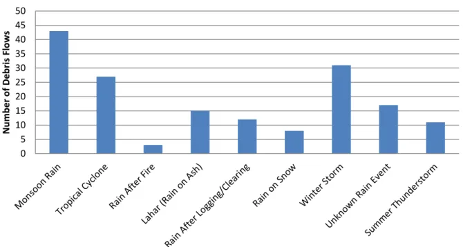
The following graphs present the results on triggers and causes of fatal debris flows. Figure 4.21and Figure 4.22 compare the overall causes and triggers, while Figure 4.23 and Figure 4.24 compare triggers and causes specifically from rainfall. One hundred sixty five events from the database contain information on the trigger and cause of fatal debris flows.

Figure 4.21: Graph of the number of fatal debris flows by the cause/trigger.

Figure 4.22: Graph of the median number of fatalities per debris flow by cause/trigger.

0 20 40 60 80 100 120 140 160 Landslide Mobilised into Debris Flow GLOF Volcano Flank Collapse Landslide Dam Burst Rapid Snowmelt Mine Dump Failure Earthquake Lahar (Glacier Melt/Crater Lake) Rainfall Event N u m b e r o f D e b ri s Fl o ws

Number of Debris Flows by Cause/Trigger

1 10 100 1000 Landslide Mobilised into Debris Flow GLOF Volcano Flank Collapse Landslide Dam Burst Rapid Snowmelt Mine Dump Failure Earthquake Lahar (Glacier Melt/Crater Lake) Rainfall Event M e d ian N u m b e r o f Fatal ities p e r Ev e n t

Figure 4.23: Graph of the number of fatal debris flows triggered/caused by rainfall induced events.

Figure 4.24: Graph of the median number of debris-flow fatalities by rainfall induced cause/trigger. 0 5 10 15 20 25 30 35 40 45 50 N u m b e r o f D e b ri s Fl o ws

Number of Debris Flows by Rainfall Induced Cause/

Trigger

Median Number of Fatalities based on Rainfall Cause/

Trigger

4.4.4 Debris-Flow Volume

This section contains the results of the regression analysis for the relationship between debris-flow volume and fatalities. Table 4.2 provides data from the F test while Figure 4.25 and Figure 4.26 contain the results for the regression analysis. Figure 4.27 provides four regressions, one for each population class as defined in Table 3.2. Volume data was collected for 66 debris flows.

Table 4.2: Volume Regression F Test Results Source Degree of

Freedom

Sum of Squares

Mean

Squares F Value P Value

Regression 1 26.7763 26.7763 34.84 0.000 Error 64 49.1857 0.7685 Total 65 75.9619 1.000 0E+1 0 1000 0000 00 1000 0000 0 1000 0000 1000 000 1000 00 1000 0 1000 100 100000 10000 1000 100 10 1 0.1 0.01

Debris Flow Volume (m^3)

N u m b e r o f Fa ta lit ie s b y E v e n t R-Sq 35.2% Regression 95% CI 95% PI Number of Fatalites Depending on Volume

log10(Fatalities) = - 0.8433 + 0.4215 log10(Volume)

Figure 4.25: Graph of number of fatalities depending on volume. The regression equation, trend line with confidence and prediction intervals, as well as the R2 value are provided.

3.5 3.0 2.5 2.0 1.5 1.0 0.5 0.0 2 1 0 -1 -2 Fitted Value R e si d u a l Versus Fits

(response is log10(Volume Fatalities))

Figure 4.26: Residual versus fits plot for fatalities versus volume regression.

Figure 4.27: Line graphs of debris-flow fatalities depending on volume based on the population. The R2 values and the regression found by Minitab are provided in the key for each population size.

4.5 Socioeconomic Results

The results of the socioeconomic analysis were subdivided by indicator. Each indicator includes a table of F Test results, a graph of the regression, and the residuals versus fit plot for

0.1 1 10 100 1000 10000 100000 1 100 10000 1000000 100000000 1E+10 Fatal ite s p e r Ev e n t Volume (m^3)

Debris-Flow Fatalities Depending on Volume based on

Population

the regression. The final subsection includes the histograms and descriptive statistics for developing and advanced countries as classified by the IMF.

4.5.1 GDP per Capita Regression

This subsection contains the results of the GDP per capita regression. Table 4.3 provides the results for the F Test, Figure 4.28 provides a graph of the regression, and Figure 4.29

provides the residuals versus fit plot.

Table 4.3: Gross Domestic Product per Capita Regression F Test Results Source Degree of

Freedom

Sum of Squares

Mean

Squares F Value P Value

Regression 1 21.233 21.2327 27.51 0.000 Error 210 162.058 0.7717 Total 211 183.290 100000 10000 1000 100 100000 10000 1000 100 10 1 0.1 GDP per Capita N u m b e r o f Fa ta lit ie s b y E v e n t R-Sq 11.6% Regression 95% CI 95% PI Number of Fatalites Depending on GDP per Capita

P = 0.000

Figure 4.28: Graph of the relationship between fatalities per debris flow and GDP per capita. The P value, trend line with confidence and prediction intervals, as well as the R2 value are provided.

2.25 2.00 1.75 1.50 1.25 1.00 3 2 1 0 -1 -2 Fitted Value R e si d u a l Versus Fits

(response is log10(GDP per Capita Fatalities))

Figure 4.29: Residual versus fits plot for fatalities versus GDP per capita regression.

4.5.2 Hospital Beds per Capita Regression

This subsection contains the results of the hospital beds per capita regression. Table 4.4 provides the results for the F Test, Figure 4.30 provides a graph of the regression, and Figure 4.31 provides the residuals versus fit plot.

Table 4.4: Hospital Beds per Capita Regression F Test Results Source Degree of

Freedom

Sum of Squares

Mean

Squares F Value P Value

Regression 1 13.329 13.3294 17.73 0.000

Error 133 99.990 0.7518

10 1 0.1 100000 10000 1000 100 10 1 0.1

Number of Hospital Beds per 1,000 Citizens

N u m b e r o f Fa ta lit ie s b y E v e n t R-Sq 11.8% Regression 95% CI 95% PI

Number of Fatalites Depending on Number of Hospital Beds

P = 0.000

Figure 4.30: Graph of the relationship between fatalities per debris flow and the number of hospital beds per capita. The P value, trend line with confidence and prediction intervals, as well as the R2 value are provided.

2.00 1.75 1.50 1.25 1.00 0.75 0.50 3 2 1 0 -1 Fitted Value R e si d u a l Versus Fits

(response is log10(Hospital Bed Fatalities))

4.5.3 Maternal Mortality Rate Regression

This subsection contains the results of the Maternal Mortality Rate regression. Table 4.5 provides the results for the F Test, Figure 4.32 provides a graph of the regression, and Figure 4.33 provides the residuals versus fit plot.

Table 4.5: Maternal Mortality Rate Regression F Test Results

Source Degree of _Freedom Sum of _Squares Mean _Squares F Value P Value

Regression 1 8.6382 8.63818 11.70 0.001 Error 111 81.9504 0.73829 Total 112 90.5886 1000 100 10 100000 10000 1000 100 10 1 0.1

Maternal Mortality Rate (per 10,000 births)

N u m b e r o f Fa ta lit ie s b y E v e n t R-Sq 9.5% Regression 95% CI 95% PI

Number of Fatalites Depending on Maternal Mortality Rate

P = 0.001

Figure 4.32: Graph of the relationship between fatalities per debris flow and MMR. The P value, trend line with confidence and prediction intervals, as well as the R2 value are provided.

1.8 1.6 1.4 1.2 1.0 0.8 0.6 3 2 1 0 -1 -2 Fitted Value R e si d u a l Versus Fits

(response is log10(MMR Fatalities))

Figure 4.33: Residual versus fits plot for fatalities versus MMR regression.

4.5.4 Life Expectancy Regression

This subsection contains the results of the life expectancy at birth regression. Table 4.6 provides the results for the F Test, Figure 4.34 provides a graph of the regression, and Figure 4.35 provides the residuals versus fit plot.

Table 4.6: Life Expectancy Regression F Test Results Source Degrees of

Freedom

Sum of Squares

Mean

Squares F Value P Value

Regression 1 8.522 8.52231 10.40 0.002

Error 145 118.871 0.81980

80 70 60 50 40 100000 10000 1000 100 10 1 0.1

Life Expectancy at Birth (years)

N u m b e r o f Fa ta lit ie s b y E v e n t R-Sq 6.7% Regression 95% CI 95% PI

Number of Fatalites Depending on Life Expectancy

P = 0.002

Figure 4.34: Graph of the relationship between fatalities per debris flow and life expectancy at birth. The P value, trend line with confidence and prediction intervals, as well as the R2 value are provided. 2.25 2.00 1.75 1.50 1.25 1.00 3 2 1 0 -1 -2 Fitted Value R e si d u a l Versus Fits

(response is log10(Life Expectancy Fatalities))

4.5.5 Corruption Perception Index Regression

This subsection contains the results of the Corruption Perception Index regression. Table 4.7 provides the results for the F Test, Figure 4.36 provides a graph of the regression, and Figure 4.37 provides the residuals versus fit plot.

Table 4.7: Corruption Perception Index Regression F Test Results

Source Degrees of _Freedom Sum of _Squares Mean _Squares F Value P Value

Regression 1 12.1498 12.1498 17.35 0.000 Error 94 65.8331 0.7004 Total 95 77.9829 10 9 8 7 6 5 4 3 2 1.5 100000 10000 1000 100 10 1 0.1 CPI N u m b e r o f Fa ta lit ie s b y E v e n t R-Sq 15.6% Regression 95% CI 95% PI Number of Fatalites Depending on Corruption Perception Index

P=0.000

Figure 4.36: Graph of the relationship between fatalities per debris flow and CPI. The P value, trend line with confidence and prediction intervals, as well as the R2 value are provided.

2.25 2.00 1.75 1.50 1.25 1.00 0.75 0.50 3 2 1 0 -1 -2 Fitted Value R e si d u a l Versus Fits

(response is log10(CPI Fatalities))

Figure 4.37: Residual versus fits plot for fatalities versus CPI regression.

4.5.6 Technical Journal Publications per Capita Regression

This subsection contains the results of the total technical journal publications per capita regression. These include all technical articles published in in various scientific fields. Table 4.8 provides the results for the F Test, Figure 4.38 provides a graph of the regression, and Figure 4.39 provides the residuals versus fit plot.

Table 4.8: Technical Journal Publication per Capita Regression F Test Results

Source Degrees of _Freedom Sum of _Squares Mean _Squares F Value P Value

Regression 1 19.3932 19.3932 29.38 0.000

Error 95 62.7033 0.6600